Blind Identification Using ARMA
model Second Order
By
Hala Alhajhasan
Supervisor
Dr Wasfi Kafri
2008
BIRZEIT UNIVERSITY
FACULTY OF
GRADUATES STUDIES
Blind Identification Using ARMA
model Second Order
By
Hala Alhajhasan
A Thesis submitted in partial fulfillment of the requirement for Masters Degree in Scientific Computing from the Faculty of Graduate Studies at Birzeit University.
Supervisor
Dr Wasfi Kafri
Birzeit, Palestine
i
To My Husband
ii
Table of Contents
Table of Contents. . . ii List of Tables. . . iv List of Abbreviations. . . .v Abstract. . . .viiiChapter 1
1 Introduction. . . 1Chapter 2
2.1 Algoritms of Blind Equalization and identification. . . 62.2 Blind Identification and Equalization in communication channels. . . 7
2.3 Blind Single Input Single Output (SISO) equalization. . . 8
2.4 Channel Equalization in QAM Data Communication system . . . 9
2.5 Popular Algorithms for blind equalizatio . . . .12
2.5.1 Sato Algorithm . . . .12
2.5.2 BUSSAGE Algorithm. . . .14
2.5.3 Stop-And-Go Algorithm. . . 14
2.5.4 Constant Modulus (Godard) Algorithms. . . 16
2.6 Convergence of Blind SCD equalizers. . . 20
2.7 Summary of Algorithms. . . 22
Chapter 3
3.1 Blind identification and equalization based on second order cyclostationary statistics . . . .24iii
3.2 Cyclostationary Signal Properties. . . .28
3.3 Time Domain Representation of Cyclostationary. . . 29
3.4 Frequency Domain Approaches. . . . . . . 31
3.5 Cyclic Autocorrelation Function. . . . 33
3.6 Cyclostationarity for Over Sampled Channel Output. . . . . .34
Chapter 4
4.1 Blind Identification of ARMA System based on Second Order Cyclic Statistics . . . 374.2 Parametric ARMA Identification Method. . . 43
4.3 Identifying Poles and Zeros. . . 45
4.4 Algorithm. . . 49
4.5 Computer Simulation Results. . . .. . . 50
Conclusion . . . . . . . . . . . . 59
iv
List of Tables
Table (1) : Overview of different blind equalization algorithms.. . . 23 Table (2): Comparison of the SOCS and HOS based methods for blind equalization domain. . .28
v
List of abbreviations
ARMA Auto-Regressive Moving-Average AWGN Additive White Gaussian Noise BER Bit Error Rate
BGR Benveniste, Goursat and Ruget BIBO Bounded-Input Bounded-Output BPSK Binary Phase Shift Keying BSS Blind System Separation
CISR Channel Side Information at the Receiver CMA Constant Modulus Algorithm
DDE Decision Directed Equalization FIR Finite Impulse Response
FM Fractionally-Spaced Equalizer FSE Frequency Modulation
GA Gradient Algorithm GD Gradient Descent HOS Higher-Order Statistics
vi IIR Infinite Impulse Response
ISI Inter-Symbol Interference LMS Least Mean Square LTI Linear Time-Invariant MIMO Maximum Likelihood MISO Mean-Squared Error ML Mean-Squared Error
MMSE Minimum Mean Square Error MMSE Minimum Mean-Squared Error MPE Minimum Phase Equivalent MSB Most Significant Bit
MSE Multiple Input Multiple Output MSE Multiple Input Single Output PAM Phase Modulation
PDF Power Spectrum Density PM Probability Density Function PSD Pulse Amplitude Modulation QAM Quadrature Amplitude Modulation QPSK Quadrature Phase Shift Keying ROC Region of Convergence
SGA Second Order Cyclostationary Statistics SGD Second-Order Statistics
vii SIMO Signal to Noise Ratio
SISO Signal to Noise Ratio
SNR Single Input Multiple Output SNR Single Input Single Output SOCS Single Output Multiple Input SOS Stochastic Gradient Algorithm SW Stochastic Gradient Descent WSS Wide Sense System
ZF Zero Forcing SER Signal Error Rate
viii
Abstract
This thesis addresses the problem of blind identification for high speed wireless digital communication systems, they are always subject to intersymbol interference (ISI) caused by channel amplitude and phase distortions. In order to improve the capacity of the channel, blind Identification without the use of pilot sequences is used.
In this theses we investigate new results that address the identification of linear rational channels based on the use of second order cyclic statistics (SOCS). It is shown that channel identification is achievable for a class of linear channels without the need for a pilot tone or training periods. Moreover, channel identification based on cyclic statistics does not preclude Gaussian or near Gaussian inputs. SNR with Gaussian distribution was possible to handle.
We also investigate the identification of linear time-invariant (LTI) ARMA systems based on second order cyclic statistics using IIR filter. We present a parametric method. The parametric method we use directly identifies the zeros and poles of ARMA channels with a mixed phase. Computer simulation illustrates the effectiveness of our methods in identifying ARMA system impulse responses, compared by the traditionally used CMA method.
We also investigated blind equalization using SOCS in order to peruse phase and speed the convergence.
1
Chapter 1
Introduction
Information bearing signals transmitted between transmitter and receiver encounter signal-altering physical channel. Examples of physical channels are telephone twisted pairs, coax cable , fiber optical guide and the atmosphere for wireless communication, the last is the concern of this theses. Each of these physical channels may cause change on the signal in form of distortion. The effects are noise, Intersymbol Interference (ISI) , a critical effect in digital communication. High speed of digital data transmission over band limited channels introduces ISI.
The wireless channel transmit the signal in form of radio signal ( harmonic wave) bearing the information in form of bits or symbols. A propagating signal through the wireless channel suffers different effects: path loss , multipath referred to reflection, scattering and diffraction (obstacles) . Therefore, the signal arrives much weaker than the transmitted signal due to the phenomena mean propagation loss, slow fading (long term fading) and fast fading (short term fading) and Doppler spread in mobile communications.
2 The effects of multipath propagation on transmitted signals in digital communication systems, is one of the major obstacles in modern digital communication systems. Multipath propagation of the transmitted signal causes ambiguity of the received signal, and with noise, significantly degrades bit error rate (BER) performance of the communication system. The distortion of the received signal due to multipath is referred to as Inter Symbol Interference (ISI). ISI channel equalization plays a key role in digital communication systems. Typically, the wireless channel introduces this distortion to the transmitted signal that can make it difficult to recover the original data. In this case, an equalizer is necessary to reduce, or ideally to completely eliminate, the introduced intersymbol interference (ISI). Conventional equalization techniques rely on the transmission of a reference (training) sequence that is known at the receiver Channel side information at the receiver (CSIR). This sequence allows adaptation of the equalizer parameters to minimize some cost function that measures the distance between the actual equalizer output and the desired reference signal. For instance, when the equalizer is implemented by means of a linear filter, the filter coefficients can be easily adapted by using the well known Least Mean Square (LMS) , which minimizes the expectation of the squared error. Training sequence misuses the resources of the wireless communication system (the channel capacity). The data throughput , bandwidth and efficiency can therefore be increased if we employ an equalizer that does not require training sequence.
3 When a training sequence is not available at the receiver, such a device is called blind equalizer. Blind methods (self-recovering or unsupervised or deconvolution) has received a great amount of attention during the last two decades because of its importance in communication systems. Many algorithms have been sucessfuliy used in blind equalization by exploitation of the source signal properties such as their statistical properties, constellation properties rather than precise knowledge of the transmitted sequence.
They use the temporal structure: finite alphabet (FA), constant modulus (CM), sub-spaces orthogonality [ 5,6] and spacial structure: dirction of arrival (DOA) [4].
Representative algorithms exploiting the statistical properties are maximal likelyhood (ML), methods based on second-order statistics (SOS) , methods based on higher-order statistics (HOS) [1, 2, 3,8], references therein and methods used Second Order Cyclostationary (SOCS) [7,9,10,8,24]. Considerable research publications has been seen in the area of blind equalization and idenification finite impulse response (FIR) channels, [1,2,4,5]. The classic solutions to blind identification and equalization problem rely on channel phase information , an important entity in signal and image processing. Phase information can be derived from the HOS of its output signal [1, 2, 7] and references there in. The motivation for use of HOS is its ability to supress Gaussian noise, because a Gaussian process has all its cumulants spectra of order n > 2 identical to zero. In other words a signal burried in a Gaussian noise, a transform to a higher-order cumulant eliminates the noise which makes HOS
4 attractive for detection/or estimation of signal parameters or even the entire signal reconstruction from cumulant spectra; HOS spectra preserves the true phase character of signals. Non-minimum phase reconstruction or system identification can be achieved in HOS domain due to the ability of polyspectra (higher order than power spectral density) to preserve both magnitude and non-minimum phase information. A third motivation that is not concerned in this theses is anlyzing non-linear systems [14]. Drawbacks of algorithms of HOS is the slow convergence compared with SOS-based methods. Non-Gaussian process also contributes to slow speed of computational algorithms and the performance of the cumulant-based approach.
Since the blind algorithms based on higher-order statistics operate at the baud rate , it may also be sensitive to uncertainties , time jitter, phase jitter , and frequency offset. On the other hand the SOS mitigate the convergence problem . Moreover, the SOS of the channel output contain some phase information of the channel output when the channel input is non-stationary process. For applications in communication systems, many types of signals exhibit a particular type of nonstationarity called SOS-cyclostationary (SOCS) [9, 10, 13]. The exploitation of SOCS has shown applications in diverse areas such as detection and filtering of communication signals, parameter estimation, direction finding, identification of non linear systems [10] .
An accurate phase reconstruction in the autocorrelation (or power spectrum ) domain can only be achieved if the signal is minimum phase. Unlike HOS, the power spectrum that sees the system as being minimum phase. At this point it is
5 worthy to include that by exploitation of cyclostationarity of the received signal (channel output) via over-sampling, we are able to identify possibly non-minimum phase channel using only SOS (or SOCS).
Unfortunately when a channel is driven by a stationary process, the power spectrum does not exhibit phase information. Moreover, it is sensitive for Gaussian noise that affects both chanel capacity and probability of error ( depend on signal to noise ratio SNR).
As summary it may be surprising that non-minimum phases systems can be identified using only the SOS of the system output. However, it is also surprising that SOCS can be used if the system is driven by a non-stationary input (process). This is indeed the case of most communication channels where the input signals are cyclostationary rather than stationary.
In this theses blind equalization and identification is tackled in frequency domain for (infinite impulse response) IIR or ARMA( auto regressive moving average system) relying on the SOCS for purpose of extracting the phase information.
6
CHAPTER 2
2.1 Algoritms of Blind Equalization and identification
Blind equalization and identification are two problems that arise in a variety of engineering and science areas such as digital and data communications, speech signal processing, image signal processing, biomedical signal processing....etc The two problems are closely related to each other, and therefore similar design philosophies may frequently apply to the design of the system identification algorithms and the equalization algorithms.
Equalization is a signal processing procedure that restores a set of distorted source signals, these source signals are distorted by an unknown linear (or non linear) system, whereas system identification is a signal processing procedure to identify and estimate the unknown linear (or non linear) system. Linear channel distortion as a result of limited channel bandwidth, multipath and fading is often the most serious distortion in digital communication systems which cause ISI. Traditionally, channel equalization is based on initial training period. Due to severe time variations in channel characteristic, as it is the case in a mobile wireless RF communication system, the training sequence has to be sent periodically to update the estimate, there by reducing the effective channel rate.
7 In addition, time-varying multipath propagation can cause significant channel fading, leading to system outage and equalizer failure during the training periods. It is therefore desirable that the channel be equalized without using training signal, that is, in a blind manner, by using only the received signal. Summarizing, blind equalization is a process during which an unknown input data sequence is recovered from the output signal of an unknown channel [1,3, 5, 8], where the transmission of a training sequence in many high data rate, bandlimited digital communication systems is either impractical or very costy. [2]
2.2 Blind Identification and Equalization in communication channels In data communications, digital signals are generated and transmitted by the sender through an analog channel to the receiver as shown in fig 1.
Fig 1 system Identification
The design of equalization algorithms is straight forward and effective when the system is completely known in advance. When the source signals and the system are unknown, the linear channel distortion affects both transmission quality (degrades the recived signal) and efficiency in wireless communications and imposes limits on data transmission rates (limit channel capacity) in many physical channels, where it became one of the most practical problems in digital
8 communications. Band limiting effect of the practical channel (when channel bandwidth is not large enough to accommodate the essential frequency content of the data stream, results in signal distortion of Intersymbol Interference (ISI). As these signals can be added destructively or constructively, causing severe ISI can arise from the time-varying multipath fading that commonly exists in a mobile communications environment. The varying channel characteristics must be identified and equalized in real time to maintain the correct flow of information. The channel identification and equalization technique currently used requires a major fraction of the channel capacity to send a training sequence over the channel. It should be noted that while the density of mobile users in a given city area is likely to increase dramatically, the number of radio channels in that area remains constant. Although many techniques, can be used to increase the channel capacity, the fraction of the channel capacity currently used for channel identification and equalization is very considerable. To save this fraction of channel capacity, blind channel identification is an attractive approach. Using the blind channel identification techniques, the receiver can identify the channel characteristics and equalize the channel based on the received signal. No training sequence is needed, which saves the channel capacity.
Blind equalization is usefull to cancel the repeatedly transmitted training signals to improve system throughput, as the transmission of training signals obviously decreases communications throughput A reliable blind equalization algorithm is needed to be established that garantee speedy convergence, simpler and
9 effective computation, efficient that can compete with training based algorithms [1, 2, 11].
2.3 Blind Single Input Single Output (SISO) equalization
Blind equalization has four classes ; Single Input Single output (SISO), single input multiple output (SIMO), Multiple Input Single Output (MISO) and the most representative of all classes is theMultiple Input Multiple Output (MIMO). Many blind equalization algorithms have been designed to extract digital communications signals corrupted by inter-symbol interference. In the general blind equalization task the source signal filtered by an unknown transmission channel, denoted by with unknown impulse response. The question is how to recover the input signal from the output without assistance of a training sequence when the channel is unknown.
In this theses We will study the basics of blind equalization for SISO discrete systems and will describe commonly used blind algorithms highest important issues regarding their convergence.
Most blind equalization schemes begin by sampling the channel output at the baud rate (needs perfect timing recovery) to produce a stationary channel output sequence for processing or fractionally sampled (higer rate than the baud rate)[1, 2].
2.4 Channel Equalization in QAM Data Communication system
In data communication, digital signals are transmitted through an analog channel to the receiver. Considering pulse amplitude modulated (PAM)
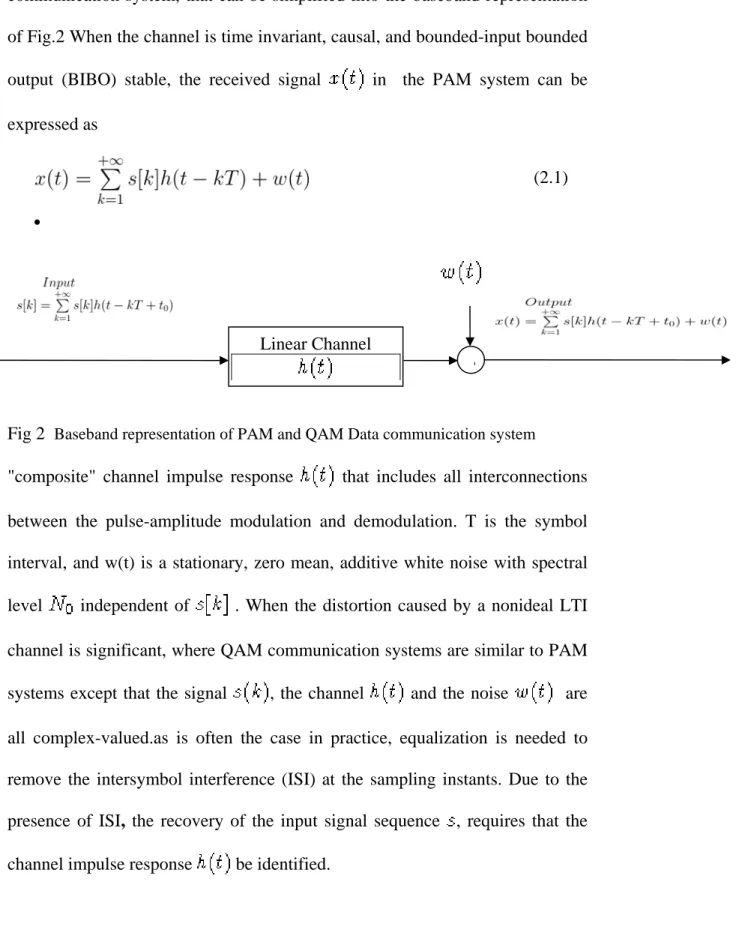
10 communication system, that can be simplified into the baseband representation of Fig.2 When the channel is time invariant, causal, and bounded-input bounded output (BIBO) stable, the received signal in the PAM system can be expressed as
(2.1)
•
Fig 2 Baseband representation of PAM and QAM Data communication system
"composite" channel impulse response that includes all interconnections between the pulse-amplitude modulation and demodulation. T is the symbol interval, and w(t) is a stationary, zero mean, additive white noise with spectral level independent of . When the distortion caused by a nonideal LTI channel is significant, where QAM communication systems are similar to PAM systems except that the signal , the channel and the noise are all complex-valued.as is often the case in practice, equalization is needed to remove the intersymbol interference (ISI) at the sampling instants. Due to the presence of ISI, the recovery of the input signal sequence , requires that the channel impulse response be identified.
Linear Channel
+
11 Although Intersymbol interference arises in quadrature amplitude modulation (QAM), However its effect can be most easily described for a baseband pulse-amplitude modulation (PAM) system[7].
In blind equalization, The transmitter generates a sequence of complex-valued random input data which is unknown to the receiver except for its probabilistic or statistical properties over the known alphabet (or constellation) of the QAM symbols .which is real for PAM and complex for quadrature amplitude modulation QAM. Usually, this signal constellation is symmetric, resulting in symmetric statistics for the i.i.d. input data. Thus, typical QAM data communication system, simply consists of a linear unknown channel which represents all the inter-connections between the transmitter and the receiver. The data sequence is sent through a linear channel whose output is received by the receiver. The function of the blind equalizer at the receiver is to estimate the original data from the received signal
by outputting a sequence of estimates for .
The complex-valued LTI communication channel is assumed to be linear and causal with impulse rerponse . The input/output relation of the QAM system can be written as
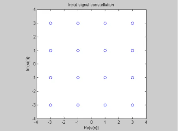
PAM is typically visualized in a constellation diagram .In which the input symbol is uniformly distributed on the following M-levels,
12
Fig 3 16-QAM complex-valued symbol set, in which the input signal {-3, -1, 1, 3} + j*{-3, -1, 1, 3}
Generally, a communication channel can be represented by a filter as depicted in Fig 2 The transmitted data symbols belong to a finite alphabet , which
can be defined as as shown in
fig 3
2.5 Popular Algoithms for Blind Equalization
The first blind channel equalization methods were based on a single-input single-output (SISO) channel models, sampled at the symbol rate. Some of them, such as the constant modulus algorithms (CMAs), involve nonlinear optimization and higher-order statistics (cummulants) of the channel output. Accurate estimation of cummulants requires large sample sizes. Although non-minimum-phase SISO channel is invertible by an infinitely long equalizer, 2.5.1 Sato Algorithm
Sato was the first to develop a blind equalizer recursive algorithm for multilevel PAM signals, when the PAM input is binary 1975 [17].
13 The Sato adaptive algorithm was one of the first widely used recursive identification schemes for discrete time system inverse identification based on measuring the system output without explicit knowledge (i.e., direct measurements) of its input . The only information concerning the system input utilized by the algorithm was knowledge of its statistical properties, e.g. the input probability distribution.
. The error function is then given as
(2.3) where is defined as
(2.4)
Where denotes the statistical expectation the parameter vector is updated via
(2.5)
(2.6)
where represents the vector of input signals at iteration step .
The generalized algorithms have been shown to possess a desirable global convergence property under two idealized conditions. The convergence properties of this class of blind algorithms under practical constraints common to a variety of channel equalization applications that violate these idealized conditions are studied. Results show that, in practice, when either the equalizer is finite-dimensional and/or the input is discrete (as in digital communications)
14 the equalizer parameters may converge to parameter settings that fail to achieve the objective of approximating the channel inverse[1].
2.5.2 BUSSAGE ALGORITHM
The output signal of the linear equalizer is defined as
(2.7)
where is a scalar function of the equalizer output, which is preferably even to distinguish between ± levels.
Merely the designed equalizer is a minimum ISI equalizer since we penalize ISI and try to optimize the coefficients to minimize ISI in which the mean cost function should be specified such that at its minimum. Stochastic gradient descent minimization algorithm for an arbitrary cost function is given as
(2.8)
Thus we want to define the derivative of the error function as
(2.9)
2.5.3 Stop-And-Go Algorithms
To avoid convergence to local minima in the cost function(poor performance) Picchi and Prati invented“stop-and-go” methodology, the Idea is to continue adapting the filter when error function is more likely to have the correct sign for
15 the gradient descent direction.Example:Consider two algorithms with error functions and , respectively. “Stop-and-Go” would mean
(2.10) Error functions and should be selected such that they maximize
reliable regions and make most of the local and the global knowledge of the constellation. Given the equalizer output , the closest symbol
can be considered as a local information; while the size (number of alphabets), shape (square or cross) and energy (mean distance between the symbols) of the constellation can be considered as global information. is termed local as it may change from one output to another; while the size, shape and energy are fixed and don’t depend on any specific value of . Most of the stochastic gradient descent algorithms employ error functions
which exhibit global information. They compute an estimate of , by doing some nonlinear operation on the current equalizer output such that the certain statistics of are forced to match with global statistics of the transmitted data[1].
16 2.5.4 Constant Modulas(Godard) Algorithms (app 1980)
The CMA is based on a criterion that penalizes deviations of the modulus of the equalized signal away from a fixed value determined by the source alphabet. Strikingly, CMA has also been successful in equalizing sources not possessing a constant modulus property, such as QAM constellations. Hence, CMA is a method that may be applied over the majority of radio communication signals. The first major study of the CMA and its properties was performed by Treichler et al. who analyzed the capture and lock behavior of baud-spaced CMA.
The vast majority of initial studies in blind equalization in general and the CMA method in particular have considered noise-free channels since it was argued that ISI is the major reason for signal degradation.
This argument does not always hold in wireless channels where the channel medium cannot be controlled as effectively. However, in wireless channels, multiuser interference, atmospheric noise (thunderstorms), car ignitions, and other types of naturally occurring or man-made signal sources result in an aggregate noise component that may exhibit high amplitudes for small duration time intervals .
The Godard algorithms which is also known as constant modulas algorithm(CMA) are a different generalization of the Sato Algorithm by Godard .It developed independently by Treichler et al.as the CMA, the most popular scheme for blind equalization of QAM systems. Integrating Sato’s error function yields.
17 (2.11)
This cost function was generalized by Godard into another class of algorithms that are specified by the cost function
, (2.12)
where is defined as
(2.13)
Resulting in an update equation
(2.14)
for the special case of q = 2 the algorithm is called “Constant Modulus Algorithm”, i.e. the channel signal has a constant modulus
to attain perfect equalization. The Godard algorithm(GA) adjusts the equalizer parameter by minimizing the Godard cost function defined as
(2.15) The cost function of CMA is of the form:
(2.16)
Where indicates statistical expectation. is the constant depending only on the input data symbol . It is defined as
(2.17)
is the equalizer output given by y[k] where is the equalizer tap weights vector,
18
(2.18)
let be the pth-order cumulant of defined as
(2.19) The stochastic gradient algorithms are defined by minimizing the cost function
subject to where (2.20)
Adaptive algorithms are typically obtained as stochastic gradient descent method to minimize the cost function. Given a cost function that can be written as
(2.21)
an on-line adaptive equalization algorithm adjusts the parameters of the equalizer via
(2.22) Here, is a small adaptation step size, and is sometimes referred to as the error function.
CMA penalizes all signals which are not constant modulus, equalization and carrier recovery are independent. A carrier frequency offset causes phase rotation of the output
(2.23)
CMA cost function is insensitive to the phase. Possible application of CMA in analog modulation signals such as FM or PM.
19 The Godard cost function has length-dependent local minima, but it has no cost-dependent local minima ,also has a one-to-one correspondence exists between the minima of the Godard algorithms.
Although some convex cost functions can be designed for adaptive blind equalizers under specific parameter constraints to avoid local convergence, these algorithms tend to be rather slow due to their , nature of the cost functions. Moreover, all the above convergence analyzes of blind algorithms are based on the noiseless channel assumption for analytical simplicity. There are no analytical results under noise yet. In fact, there have been some conjecture that channel noises may help equalizer parameters to escape some shallow local minima. Since channel noise is present in all practical communication systems even it is often small, convergence analysis of blind equalization algorithms must be carried out under channel noise.
The blind equalization of a non minimum phase system requires necessarily a non linear transformation over the sequences involved in the adaptation process. Whereas the Godard class has smooth cost functions, the BGR algorithms have been particularly difficult to analyze because of a discontinuity appearing in the prediction error of the adaptation algorithm . In contrast, the smooth Godard algorithms have been successfully analyzed recently [20]
Sato and Godard approach the problem of blind equalization by introducing new criteria, different from the mean-square error (MSE) criterion used for trained equalizers, and then apply a gradient-search algorithm to optimize the selected criterion. These methods converge to the desired response under certain
20 assumptions concerning the probability distribution of the input sequence for the analysis and extension of Sato’s method and for the analysis of Godard’s method.
Benveniste er al. present several concepts and results that significantly contribute to the understanding of the problem. First, they establish that a criterion based on second-order statistics, e.g., the MSE criterion, is insufficient for phase identification. For that reason the problem cannot be solved when the input distribution is Gaussian, since second-order moments completely specify the input-output statistics. Next, it has been proved that a sufficient condition for equalization is that the probability distribution of the individual recovered symbols , be equal to the probability distribution of the individual input symbols .
Among many important findings in, it was shown that if the channel input is sub-Gaussian, then these algorithms exhibit ideal global convergence properties. Algorithms using implicit HOS are called Bussgang-type , such as the well-known Godard and Sato algorithms. HOS techniques usually suffer from their slow convergence and local minima problems. Algorithms based on SOS mainly exploit matrix decomposition methods[21].
2.6 Convergence of blind SCD equalizers
What measures the success of the blind equalizer algorithm? Thus to design a satisfactory algorithm that acheives the goal of blind equalization “the desired convergence for noisless channels. the algorithm should result in the convergence of equalizer parameters to equilibria that can eliminate sufficient
21 ISI.under the QAM enviroment ie. the function has to be selected such that the local minima of correspond to significant removal of ISI. A possible equilibrium of the blind equalizer.If the input constellaion is knwon to the receiver then it dictates the acceptable removal of ISI, which in turn determines the acceptable convergence performance of blind equalizer.,the more we know about the constellation, the more relaxed the convergence performance of algorithm can be.
(2.24) where is the stepsize of the algorithm.
(2.25) We notice that the distribution and the constellation of the input sequence affect the convergence of blind equalizer.
We notice that the stable stationary points of equation 2.5.6 correspond to the local minima:
(2.26) The geometry of the error function over the equalizer parameters determines the convergence of the adaptive algorithm,usually simulation results demonstrates the convergence of the blind algorithms and not analysis because it is dificult to do that due to the dependence of the statistical characterization of the channel output signal on the unknown channel impulse response.
Sato, BGR, Stop-and-Go, CMA, Shalvi-Weinstein Algorithm are hard to analyze convergence behavior of the algorithms.
22 Since finite parameterization is a practical necessity for terization may have undesirable minima. Undesirable local convergence behavior has been shown for the Godard algorithm (CMA case) the BGRA and the Shalvi and Weinstein Algorithm.
2.7 Summary of algorithms
In many blind adaptive algorithms, a cost function an be defined. In general but is chosen from
(2.27)
This way, the general update equation
(2.28) Table(1) below lists the algorithms most commonly used for adaptive blind equalization.
Algorithm error function /nonlinearity update equation Decision
Directed
23 Table (1) : Overview of different blind equalization algorithms.
Godard,CMA Sato (CMA) BGR Benveniste-Goursat Stop-and-Go
24
Chapter 3
3.1 Blind identification and equalization based on second order cyclostationary statistics
Blind channel equalization plays an important role in digital communication systems when the training sequence is impractical or misuse the resorces as channel capacity (e.g. mobile GSM system uses about 50% of the channel capacity for training sequence). Channel equalization requires that channel transfer function be identified. The major difficulty is that the input signal to be transmitted through the channel is not available. Hence numerical optimization methods, in particular, the method Minimum Mean Square Error (MMSE), are not applicable, therefore, special blind equalization and identification methods are needed.
Conventional algorithms for adaptive blind equalization are based on Higher Order Statistics (HOS) or Second Order Statistics (SOS). Algorithms using explicit HOS use Higher Order Cumulants (HOC). Algorithms using implicit HOS are called Bussgang-type, such as the well-known Godard and Sato algorithms. HOS techniques usually suffer from their slow convergence and local minima problems. Algorithms based on SOS mainly exploit matrix
25 decomposition methods or unsupervised neural networks for blind equalization. Both HOS and SOS based algorithms have their merits and demerits.
It has been clear that almost all man-made communication signals exhibit a statistical property called cyclostationarity. It is Shown that the second-order statistics (SOS) of a cyclostationarity signal contains the phase information of the channel thus it goes through, and this phase information can be used to identify the channel, which is possibly a non-minimum phase channel, up to a complex constant. The first blind equalizer that was proposed by using the phase information contained in the SOS of the oversampled output sequence, the blind fractionally spaced equalizer, based on the cyclostationarity and data structures involved in the oversampled received sequence. Although these methods can obtain an acceptable equalization performance within 100 or more symbols, they are generally sensitive to the error in channel order estimation. In these algorithms, it is generally assumed that the channel order is either known or can be estimated by other algorithms. As we know, when the signal-to-noise ratio (SNR) becomes smaller, to determine a correct channel order from the channel output is a difficult task. In order to weaken the dependence on channel-order estimate, in comparison with SOS, the higher order statistics (HOS) of a signal offers an appealing benefit: insensitivity to an additive Gaussian noise. This benefit is very useful in communication systems because most noises in communication system can be described approximately by Gaussian distribution. However, in order to exploit its HOS, a non-Gaussian symbol sequence with independent and identically distributed (i.i.d.) functions
26 are commonly assumed. Although the i.i.d. condition is stricter than the cyclostationarity used in SOS-based methods, two facts render it applicable: 1) the real input symbol sequence tends to be i.i.d. and 2) if the HOS is utilized only up to the fourth order, then a qualified input symbol sequence is only required to satisfy i.i.d. condition up to the fourth order (i.e., not to infinity.) Many blind channel identification and equalization methods based on HOS have been developed.
Therefore the classic tools used for channel identification and equalization rely on channel phase information derived from HOS. The motivation for use of HOS its ability to suppress Gaussian noise, because a Gaussian process has all its cumulants spectra of order n > 2 identicll to zero. In other words a signal buried in a Gaussian noise, a transform to a higher-order cumulant eliminate the noise which makes HOS attractive for detection/or estimation of signal parameters or even the entire signal reconstruction from cumulant spectra; HOS spectra preserve the true phase character of signals. Non-minimum phase reconstruction or system identification can be achieved in HOS domain due to the ability of polyspecra (higher order than power spectral density) to preserve both magnitude and non-minimum phase information. Drawbacks of algorithms of HOS is the slow convergence compared with SOS-based methods. However HOS exhibit high-variance and channel variations may violate the stationarity assumption as the receiver collects long records required for reliable HOS equalization.
27 A channel driven by a stationary process the power spectrum (PS) does not exhibit phase information. Moreover, it is sensitive for Gaussian noise that affects both channel capacity and probability of error( depend on signal to noise ratio (SNR)). On the other hand the SOS mitigate the convergence problem. Moreover, the SOS of the channel output do contain some phase information of the channel output when the channel input is non-stationary process. For applications in communication systems, many types of signals exhibit a particular type of nonstationarity called SOS-cyclostationary ( SOCS) [9, 10, 13]. An accurate phase reconstruction in the autocorrelation (or power spectrum, SOS ) domain can only be achieved if the signal is minimum phase. Unlike HOS, the power spectrum that sees the system as being minimum phase. At this point it is worthy to include that by exploitation of cyclostationarity of the received signal (channel output) via over sampling, we are able to identify possibly non-minimum phase channel using only SOS (or SOCS). In Second Order Statistics (SOS) based system identification, the autocorrelation of the output sequence is used to estimate the parameters. However since autocorrelation is phase blind, these methods cannot distinguish between minimum phase and minimum phase systems. Even if the system is non-minimum phase, those roots, which are outside the unit circle, are mapped back into the interior of the unit circle. Thus the minimum phase equivalent (MPE) of the non-minimum phase system is identified.
Note that if the driving noise is Gaussian and the system is minimum phase, then SOS based methods can identify the system correctly . If the driving noise
28 is Gaussian and the system is non-minimum phase, then no method can correctly identify the system using outputs alone. However, if the driving noise is non-Gaussian, then there exist methods based on Higher Order Statistics (HOS) which can identify the system correctly. This is because HOS preserves phase information for non-Gaussian noise, but it is phase blind for all kinds of Gaussian noise.
Table(2) below compare between SOCS, SOS and HOS.
SOCS SOS HOS
Identifiability conditions
Coprime subchannels Gaussian NonGaussian signals
Performance Fast convergence Medium -fast Slower convergence
Compexity Medium to low Medium High
Table (2): Comparison of the SOCS and HOS based methods for blind equalization domain
3.2 Cyclostationary signal property
Cyclostationarity is a useful property used in blind channel equalization and identification , it is obtained by oversampling the channel output with a frequency higher than the baud rate and used as an alternative method to HOS based methods.
Spectral correlation properties of cyclostationary signals can be used by treating their spectral correlation density functions or cyclic autocorrelation functions. A new approach has presented channel identification methods based on the use of second-order cyclic spectra of the channel output[16] presented a frequency
29 sampling method utilizing the relationship between cyclic spectra and the channel frequency response.
Many digital communications signals are cyclostationary, the continuous time channel output signal in PAM and QAM data communication systems are in fact cyclostationary processes. is it possible to achieve channel identification based solely on second order cyclic statistics of the channel input and output to recover the phase of the channel transfer function[7].
The magnitude of the channel transfer function is first derived from the power spectral density or the cepstrum of cyclic spectra, then the channel phase based on the cyclic spectra alone is reconstructed.
The cyclostationarity property is a result of the implicit periodicity of these signals, related to the baud rate,carrier frequency or any other periodic component.
Cyclostationary signals have periodically time-varying second order statistics, they have a periodic autocorrelation, while stationary signals have second order statistics which are constant with time.
In the following section we will present the cyclostationarity in time and frequency domain.
3.3 Time Domain Representation of Cyclostationary
To analyse cyclostationary signals, we start by comparing the two parameter cyclic autocorrelation with the more conventional autocorrelation function. Periodicity of this function with time results in spectral redunduncy which can
30 be exploited by advanced signal processing methods to give an enhanced immunity of a signal to interference.
Autocorrelation is a measure of how closely a signal, or sequence, is correlated with time shifted versions of itself. Two relatively time shifted versions of the signal are multiplied together and then some form of avaraging is used to give a result which is a function of time or time shift.
A wide sense stationary signal or process is one in which the mean value and autocorrelation are invariant in time. The autocorrelation of a random process is the expected value of the product expressed mathematically as:
(3.1)
Or
(3.2)
Where E[.] indicates the expected value.
Wide sense cyclostationary signal or process is one in which the mean value and autocorrelation are periodic, using the probabilistic definitions :
(3.3) (3.4)
(3.5)
Where is an integer. The subscript on indicates that is the autocorrelation of the signal is the probabilistic autocorrelation function expressed as a function of two variables, and where is a
31 “parametric time” (the lag between the two signals) , and is ” real time”, (the time origin of the autocorrelation calculation )
In equation (3.3), autocorrelation function is periodic in with period . That is the fundemental period is , and is also periodic at harmonics of . The properties of autocorrelation (and mean) based on the probabilistic definition are of course dependent on how the ensemble is defined. An ensemble is an imaginary set of an infinite number of instances of the process or under consideration, but it is important to be aware of the similarities and differences between these different instances.
As the duration of a finite signal increases, the finite deterministic autocorrelation function obviously tends towards the infinite deterministic autocorrelation. As time tends to , the deterministic autocorrelation tends towards the probabilistic autocorrelation as long as the signal or process is ergodic.
3.4 Frequency domain approaches
Frequency domain approaches rely on cyclic spectra of the channel output explicitly, when the channels has limited phase variations (e.g channels with rational transfer functions), the channel dynamics can be identified through the use of cyclic spectra of the cyclostationary channel output signal. The channel output signal should be sampled at higher rate than the baud rate which will have important second order statistical information for linear channel identification.
32 QAM signals exhibit cyclostationarity related to the baud rate. The baud rate related to correlation can be seen to be a direct result of the sampled signals properties :
Let be a continuous time signal which changes instantaneously, at random times, between the values ( , It has equal probability of taking each of these two values. The signal changes in such that at every instant, it is uncorrelated with every other instant. This purely real, signal is chosen because it is simple to be represented graphically.
A sequence of impulses carrying data values of can be constructed by multiplying by sampling function which is a sequence of impulses:
(3.6)
(3.7) , and FT are respectively written as:
, (3.8)
where is an integer, is the symbol period.
, (3.9)
the spectrum is invariant under frequency shifts of and made up of
aliased copies of the spectrum , so the spectrum exhibits spectral correlation.
33 An impulse sequence has a spectrum of infinite bandwidth. If a signal’s bandwidth is no greater than the Nyquist limit, then there is no cyclostationary, such a signal is stationary. To maintain a cyclostationary signal spectral correlation., we use a sufficiently high sampling frequency to exhibit baud rate. 3.5 Cyclic autocorrelation function
Cyclic autocorrelation function :
As equation (3.7) is periodic in , we can write it in the form of a Fourier series expansion:
(3.10)
The summation can be over all values of although the coefficient will be zero unless is equal to a period of the autocorrelation function. For example if
the baud rate is is a cyclic frequencies, then will take values
because the baud rate harmonics are also cyclic frequencies. If is not periodic, then all coefficients of the summation will be zero except for . If there is periodicity present then at least one other will be non-zero.
Auseful way of displaying the cyclostationarity properties of a signal is to plot the spectral correlation density (SCD). This function is defined as the fourier transform of the cyclic autocorrelation function as follows:
(3.11) The conjugate SCD is similarly defined:
34 The cyclic autocorrelation function and spectral correlation density Fourier transform pair for cyclostationary signals to the autocorrelation function and power spectral density pair for stationary signals.
In digitally modulated signals, the cyclic frequencies are usually related to the baud rate and the carrier frequency. Spread spectrum signals may have additional cyclic frequencies, as an example, a rectangular pulse BPSK signal with baud rate and carrier frequency has cyclic frequencies
3.6 Cyclostationarity for Over Sampled Channel Output
Usually blind equalization in digital communication systems is solved by using second order statistics signals sampled at the baud rate, but communication channels are, in general, nonminimum phase,which makes second order statistics approaches inadequate for channel equalization, as it is phase blind and cannot determine channel phase.
By oversampling the channel output with a frequency higher than the baud rate, we obtain a discrete cyclostationary process. Let the sampling interval be
The oversampled discrete time signal can be written as
35 Where
(3.14) (3.15)
The correlation function of is defined as
(3.16)
\Since and are independent, straightforward calculation yields
(3.17)
Clearly, is a cyclostationary process with period p since
for all (3.18) Although we assumed that is white, our basic derivation can be easily extended to colored stationary noises.
The cyclic correlation function of discrete process is defined as
(3.19)
for The cyclic spectrum of is hence obtained through
(3.20)
Equivalently, in the Z- domain, we define
36 with a channel transfer function
(3.22)
By refering to (3.22), we see that
(3.23) or
(3.24)
37
Chapter 4
4.1 Blind identification of ARMA systems based on second-order cyclic statistics
Linear parametric models of stationary random processes whether signal or noise, have been found to be useful in a wide variety of signal processing tasks such as signal detection, estimation, filtering, and classification, and in a wide variety of applications such as digital communications, automatic control, radar and sonar, and other engineering disciplines and sciences. Parsimonious parametric models such as AR, MA, ARMA or state-space, as opposed to impulse response modeling, have been popular together with the assumption of Gaussianity of the data. Linear Gaussian models have long been dominant both for signals as well as for noise processes. Assumption of Gaussianity allows implementation of statistically efficient parameter estimators such as maximum likelihood estimators. A stationary Gaussian process is completely characterized by its second-order statistics (autocorrelation function or equivalently, its power spectral density { PSD) and it can always be represented by a linear process. Since PSD depends only on the magnitude of the underlying transfer function, it does not yield information about the phase of the transfer function.
38 Determination of the true phase characteristic is crucial in several applications such as seismic deconvolution and blind equalization of digital communications channels. Use of higher-order statistics allows one to uniquely identify non-minimum-phase parametric models. Higher-order cumulants of Gaussian
processes vanish, hence, if the data are stationary Gaussian, a minimum-phase (or maximum-phase) model is the 'best' that one can estimate. Given these facts, it has been of some interest to investigate the nature of the given signal: whether it is a Gaussian process and if it is non-Gaussian, whether it is a linear process. Recent work has presented novel techniques that exploit cyclostationarity for channel identification in data communication systems. In this theses we will discuss the identification of ARMA modeled IIR channels based on cyclostationarity of the channel output signal sampled at frequency higher than the baud rate. Blind system identification can be classified into parametric and non-parametric identification. In parametric identification, the system is assumed to a particular class of models, indexed by a set of parameters. The parameters are identified from the available data. i.e. it directly identifies the poles and zeros of the mixed phase ARMA channels using SCD of the channel output with a mixed phase. In non-parametric identification an exact model of the system is not specified. Rather some assumptions are made regarding the system ( e.g, linearity assumption) and the transfer function of the system is estimated.. The parametric method requires advance information about the order of the system. Also to reduce the phase estimation errors at the poles, a hybrid method in which the poles of the channel are predetermined.
39 In general by comparing the parametric method to the nonparametric methods, the performance of a parametric method is limited to the high signal-to-noise ratio condition and is applicable only when the assumed model matches the process under consideration.
The major dificulty in identifying the channel response from second order statistics is the limited amount of phase information available from second order cyclostationary statistics and the limited support of cyclic spectrum of strictly bandlimited channels. To determine the channel phase, the channel must be finitely parametarized.
Properties of SOS that states that the SISO LTI system is absolutely summable and the source signal is a wide sense system(WSS) white process with variance , then the random signal given by
(4.1) In section 2.4 we introduced the mathematical model to describe the identification method of pulse amplitude modulated (PAM) communication system(equation 2.1).
The actual channel output is cyclostationary and is wide-sense since ( 4.2) And
( 4.3) It can be verified that
40 (4.4) Here we will test the feasibility of phase identification using second-order cyclic statistics.
The cyclic autocorrelation function for cyclostationary process with fundamental period T is defined by
(4.5)
Correspondingly, the spectral-correlation density (SCD) is given by
(4.6)
For the PAM signal of (2.1) under white channel input of unit variance, the SCD can be shown to relate to the frequency response of the channel through the expression
(4.7)
in which is the channel frequency response. Equivalently in the domain we define
(4.8) Then we denote the channel transfer function as
(4.9) So we get
41 This is the equation that we will use in our analysis and design of channel identification based on second order statistics.
The magnitude of can be identified from the Power Spectral Density (PSD) of the channel output, we have to identify the phase of from
(4.11)
correlated channel inputs if the correlation is known. Let be the phase
of SCD , and let be the phase of the frequency response ). For , the following relationship between the two phases can be written as
(4.12) For an arbitrary channel, the above equations indexed by k, in which phase unwrapping is necessary to obtain ,are the only possible sources of phase information. The identifiability of from can be better illustrated through a cepstral approach. Let
(4.13)
(4.14)
And
(4.15) From this particular relationship, we can make the following observations: No cepstral channel phase information can be extracted when
42 or when (4.16) Therefore, an arbitrary channel transfer function cannot be completely identified from the cyclostationary statistics alone.
It is clear from equation (3.5) that no additional phase information can be extracted from the SCD by setting
Consequently, we simply consider the use of SCD with that has the largest support region.
Theoretically, most of the imaginary cepstrum of can be identified through
(4.17)
except for . If is bounded at , the -normed error between the true phase and the phase estimate will be zero since the set has zero measure. However, when is not bounded at , the channel phase cannot be determined even theoretically.
For example, if has an impulse at , then correspondingly, will contain a sinusoidal part with frequency ( e.g., ) and the
-normed phase error can be infinite. It is in fact clear from (3.2) that the SCD contains no information about any oscillatory phase content with frequency
. This fact is reinforced in where it is shown that discrete channels with certain number of zeros uniformly spaced in a circle (resulting in oscillatory phase content) cannot be identified.
43 The SCD phase can only be extrapolated for all frequencies when the channel is finitely parametrized or can be well approximated by a finitely parametrized model. Thus, ARMA finite parametrization is a sufficient condition for the unique identification of channel phase from second-order cyclostationary statistics.
If nonparametric methods are used, the nonparametrized linear system cannot be uniquely determined. In that case, we must devise a strategy to remove the ambiguity without generating unreasonably large errors.
we will present methods for Blind identification of ARMA systems based on second-order cyclic statistics using the parametric method.
4.2 Parametric ARMA Identification Method
The major difficulty in identifying the channel response from second-order statistics is due to the limited amount of phase information available from second-order cyclostationary statistics and the limited support of the cyclic spectrum for strictly bandlimited channels. To uniquely determine the channel phase, the channel must be finitely parametrized. We shall assume that the channel H[z] can be well approximated by an ARMA model. Our objective of blind channel identification is then to identify the ARMA channel response from information contained in the relationship of
(4.18)
or the cyclic spectra
44 The parametric method that will be presented directly identifies the poles and zeros of the channel transfer function H[z] from its relationship with the cyclic spectra(2). We exploit the information contained in
and , which are the cyclic spectra with the largest support and are therefore the most reliable.The ARMA channel transfer function can be written as
(4.20)
where this method for channel identification is based on the following relationships: (4.21) (4.22) equation (4.2.1) is based on (4.23)
To identify the zeros of H[z] as common zeros, the zeros of the channel are among the common zeros of and , the poles of the channel are
the stable poles of or that is when there is no pole/zero cancellation in the two products of
45 It is required that no common zeros exist between and
, also zeros with the same radius must not have a phase difference of . this condition prevent cancellation of the same pole in both
and .
Based on the above, we can identify the poles and zeros;
4.3 Identifying the Poles and Zeros
Based on cyclic spectra and this simple condition that zeros on the same radius must not have phase difference of , we can identify the poles of the system as union of stable poles of and . The un-canceled zeros of the system can be identified as common zeros of and . The remaining task is to locate the common zeros that are canceled in either
or but not in both.
To find those cancelled zeros, we rely on the channel poles that have been identified. Denote the set of stable poles of as and the set of the stable poles of as . The poles of the channel are given by
(4.24) For every element in
(4.25) There is a canceled zero at
46
(4.26)
In addition, for every element in
(4.27) There is a canceled zero at
(4.28) To identify poles and zeros we have to assume that the channel must be casual, stable and time-invariant and must satisfy the following conditions:
Zeros on a circle do not have phase difference of . There are no zeros or poles on the unit circle.
Then, the poles of the ARMA system can be found as the union of roots of
(4.29) In which ‘s are determined by equations
(4.30)
For Where
(4.31)
The un-canceled zeros inside the unit circle can be found as the common roots of
(4.32) In which is determined by equations
47 (4.33) For Where (4.34)
The un-cancelled zeros outside the unit circle are the reciprocals of the remaining roots of multiplied by . The canceled zeros can be found from identified poles based on
(4.35) And
(4.36) Based on Prony's method and if is a rational function then consider the equation
(4.37)
Where is the inverse discrete Fourier transform of . For non negative integer and the poles ’s of with multiplicity .
If
(4.38)
48 We conclude that ’s are distinct and nonzero and ’s are also nonzero,
then are roots of
(4.39) With multiplicity , to determine ’s, we us the following equation
(4.40) Estimating SCD: First, estimate correlation function by
(4.41) Then, calculate cyclic correlation function
(4.42) And the cyclic spectrum by
(4.43) Identifying Channel: For the parametric algorithm, identify the poles and zeros by identifying prony’s matrix
Calculating Channel Response and NMSE: For the parametric algorithm, obtain the frequency response of the channel by:
49 4.4 Algorithm
To demonstrate the performance of the ARMA identification algorithm, several channels are tested, also the simulation is done by taking the following steps:
1) Generate the PAM data output: where =4 is the
oversampling rate. The input sequence is an i.i.d. four-level PAM signal. Is a stationary white Gaussian noise. Oversampling the input sequence gives the equivalent oversampled channel output.
2) Estimate the SCD of the received sequence: estimate the correlation function using equation 4.41, then calculate the cyclic correlation function
using equation 4.41
and the cyclic spectrum using equation 4.43
3) Identifying the channel for the parametric algorithm, identify the poles and zeros
To test four ARMA systems for our identification methods. Use identification results using the parametric under SNR =25 dB
4) Calculating Channel Response and NMSE: For the parametric algorithm, obtain the ARMA channel transfer function
50 4.5 Computer Simulation results
We test several ARMA systems for our identification method, to pick zero and pole locations, plot impulse response, plot some samples from a simulated ARMA series, plot the frequency response function.
The simulation was done under SNR=25 d B
1)We tested the channel with one pole and one zero, for 500 samples. And the following channel transfer function results.
coefficients in AR form:-0.61842, coefficients in MA form:0.4693
a) b) c) d) -1.5 -1 -0.5 0 0.5 1 1.5 -1.5 -1 -0.5 0 0.5 1 1.5
Click to place one zero at the the x component of the selection (zero of θ(z))
0 50 100 150 200 250 300 350 400 450 500 0 1 2 3 4x 10
104 impulse response : shows the filter weights
0 50 100 150 200 250 300 350 400 450 500 -8 -6 -4 -2 0x 10 104 theta: 1.00 2.13 phi: 1.00 -1.62
500 samples of ARMA(1,1) simulation
0 1 2 3 4 5 6 7 0 0.5 1 1.5 2 2.5 3 3.5 4 4.5 0 ≤λ < 2π theta: 1.00 2.13 phi: 1.00 -1.62
spectral density - linear scale
0 1 2 3 4 5 6 7 10-2 10-1 100 101 0 ≤λ < 2π theta: 1.00 2.13 phi: 1.00 -1.62
51
e) f)
g)
Fig (4.1) a) pole) coefficients in AR form are(-0.61842) and zero coefficient in MA form is (0.4693) for 500 samples. b) Impulse response. c) spectral density. d) log scale spectral density. e) spectral CDF. f) smoothed periodogram of ARMA. g) ACF of ARMA
2) We tested the channel with one pole and one zero, for 1000 samples. And the following channel transfer function results.
the coefficients in AR form -0.9693, coefficients in MA form 0.9342
a) b) 0 1 2 3 4 5 6 7 0 2000 4000 6000 8000 10000 12000 14000 16000 0 ≤λ < 2π theta: 1.00 2.13 phi: 1.00 -1.62
spectral CDF - linear scale
0 50 100 150 200 250 300 350 400 450 500 10205
10206 10207
smoothed periodogram of ARMA(1,1) simulation
0 20 40 60 80 100 120 140 0 1 2 3 4 5 6x 10
206 ACF of ARMA(',int2str(NP),int2str(NZ) simulation
-1.5 -1 -0.5 0 0.5 1 1.5 -1.5 -1 -0.5 0 0.5 1 1.5
Click to place one zero at the the x component of the selection (zero of θ(z))
0 100 200 300 400 500 600 700 800 900 1000 0 2 4 6 8x 10
13 impulse response : shows the filter weights
0 100 200 300 400 500 600 700 800 900 1000 -5 0 5 10 15x 10 13 theta: 1.00 1.07 phi: 1.00 -1.03
52 c) d) e) f) g)
Fig (4.2) a) pole coefficients in AR form are (-0.9693) and zero coefficient in MA form is (0.9342) for 1000 samples. b) Impulse response. c) spectral density. d) log scale spectral density. e) spectral CDF. f) smoothed periodogram of ARMA. g) ACF of ARMA
3) Testing for 2 poles and 1 zero for 3000 samples, coefficients in AR form -1.7456 0.87585, coefficients in MA form: 0.92544 giving the channel response 0 1 2 3 4 5 6 7 0 100 200 300 400 500 600 700 0 ≤λ < 2π theta: 1.00 1.07 phi: 1.00 -1.03
spectral density - linear scale
0 1 2 3 4 5 6 7 10-4 10-3 10-2 10-1 100 101 102 103 0 ≤λ < 2π theta: 1.00 1.07 phi: 1.00 -1.03
spectral density - log scale
0 1 2 3 4 5 6 7 0 0.2 0.4 0.6 0.8 1 1.2 1.4 1.6 1.8 2x 10 5 0 ≤λ < 2π theta: 1.00 1.07 phi: 1.00 -1.03
spectral CDF - linear scale
0 100 200 300 400 500 600 700 800 900 1000 1023
1024 1025 1026
1027 smoothed periodogram of ARMA(1,1) simulation
0 50 100 150 200 250 0 0.2 0.4 0.6 0.8 1 1.2 1.4 1.6 1.8 2x 10
53 a) b) c) d) e) f) f)
Fig (4.3) a) pole coefficients in AR form are(-1.7456 0.87585) and zero coefficient in MA form is (0.92544) for 3000 samples. b) Impulse response. c) spectral density- linear scale. d) spectral density- log scale. e) spectral CDF. f) smoothed periodogram of ARMA. g) ACF of ARMA
-1.5 -1 -0.5 0 0.5 1 1.5 -1.5 -1 -0.5 0 0.5 1 1.5
Click to place one zero at the the x component of the selection (zero of θ(z))
0 500 1000 1500 2000 2500 3000 -1
0 1 2x 10
87 impulse response : shows the filter weights
0 500 1000 1500 2000 2500 3000 -2 -1 0 1x 10 87 theta: 1.00 1.08 phi: 1.00 -1.99 1.14
3000 samples of ARMA(2,1) simulation
0 1 2 3 4 5 6 7 0 50 100 150 200 250 300 0 ≤λ < 2π theta: 1.00 1.08 phi: 1.00 -1.99 1.14
spectral density - linear scale
0 1 2 3 4 5 6 7 10-5 10-4 10-3 10-2 10-1 100 101 102 103 0 ≤λ < 2π theta: 1.00 1.08 phi: 1.00 -1.99 1.14
spectral density - log scale
0 1 2 3 4 5 6 7 0 0.5 1 1.5 2 2.5 3 3.5x 10 5 0 ≤λ < 2π theta: 1.00 1.08 phi: 1.00 -1.99 1.14
spectral CDF - linear scale
0 500 1000 1500 2000 2500 3000
10169
10170
10171
10172 smoothed periodogram of ARMA(2,1) simulation
0 100 200 300 400 500 600 700 800 -1.5 -1 -0.5 0 0.5 1 1.5 2 2.5x 10
54
4) For 2 poles and 2 zeros and 1000 samples, coefficients in AR form: -1.2018 and 0.7655, coefficients in MA form:1.2018 and 0.62438 which gives: a) b) c) d) e) f) -1.5 -1 -0.5 0 0.5 1 1.5 -1.5 -1 -0.5 0 0.5 1 1.5
Click to place a conjugate pair of zeros (zeros of θ(z))
0 100 200 300 400 500 600 700 800 900 1000 -4 -2 0 2 4x 10
58 impulse response : shows the filter weights
0 100 200 300 400 500 600 700 800 900 1000 -1 0 1 2x 10 59 theta: 1.00 1.92 1.60 phi: 1.00 -1.57 1.31
1000 samples of ARMA(2,2) simulation
0 1 2 3 4 5 6 7 0 5 10 15 20 25 30 35 40 45 50 0 ≤λ < 2π theta: 1.00 1.92 1.60 phi: 1.00 -1.57 1.31
spectral density - linear scale
0 1 2 3 4 5 6 7 10-3 10-2 10-1 100 101 102 0 ≤λ < 2π theta: 1.00 1.92 1.60 phi: 1.00 -1.57 1.31
spectral density - log scale
0 1 2 3 4 5 6 7 0 2 4 6 8 10 12x 10 4 0 ≤λ < 2π theta: 1.00 1.92 1.60 phi: 1.00 -1.57 1.31
spectral CDF - linear scale
0 100 200 300 400 500 600 700 800 900 1000 10113
10114 10115
10116