Oleg Arenz1 Mingjun Zhong2 Gerhard Neumann1 3
Abstract
Inference from complex distributions is a com-mon problem in machine learning needed for many Bayesian methods. We propose an efficient, gradient-free method for learning general GMM approximations of multimodal distributions based on recent insights from stochastic search methods. Our method establishes information-geometric trust regions to ensure efficient exploration of the sampling space and stability of the GMM updates, allowing for efficient estimation of multi-variate Gaussian variational distributions. For GMMs, we apply a variational lower bound to decompose the learning objective into sub-problems given by learning the individual mixture components and the coefficients. The number of mixture com-ponents is adapted online in order to allow for arbitrary exact approximations. We demonstrate on several domains that we can learn significantly better approximations than competing variational inference methods and that the quality of sam-ples drawn from our approximations is on par with samples created by state-of-the-art MCMC samplers that require significantly more computa-tional resources.
1. Introduction
We consider the problem of sampling or inference using a complex probability distributionp∗(x) = ˜p∗(x)/Z for which we can evaluate p˜∗(x)but not the normalization constantZ =R
xp˜
∗(x)dx. This problem is ubiquitous in machine leaning. For example, in Bayesian Inference,p˜∗(x) corresponds to the product of prior and likelihood.
As we can not sample directly from distributionp∗(x)or
1
Computational Learning for Autonomous Systems, TU Darm-stadt, DarmDarm-stadt, Germany2Machine Learning Lab, University of Lincoln, Lincoln, UK3Lincoln Center for Autonomous Systems, University of Lincoln, Lincoln, UK. Correspondence to: Oleg Arenz<[email protected]>.
Proceedings of the35th
International Conference on Machine
Learning, Stockholm, Sweden, PMLR 80, 2018. Copyright 2018
by the author(s).
use it for inference, a common approach is to use Varia-tional Inference (VI) to approximate the target distribution p∗(x)with a tractable distributionpsuch as multi-variate Gaussians (Blei et al.,2017;Regier et al.,2017) or Gaussian Mixture Models (GMM) (Miller et al.,2017; Guo et al., 2016;Zobay,2014). The optimization problem to obtain this approximation is commonly framed as minimizing the reverse Kullback-Leibler divergence (KL)
KL(p||p∗) = Z x p(x;θ) log p(x;θ) p∗(x) dx (1) with respect to the parametersθof the approximation. This objective is typically evaluated on samples drawn from p(x;θ)and optimized by stochastic optimization algorithms (Fan et al.,2015;Gershman et al.,2012). However, in order to perform the KL minimization efficiently,p(x)is often re-stricted to belong to a simple family of models or is assumed to have non-correlating degrees of freedom (Blei et al.,2017; Peterson & Hartman,1989), which is known as the mean field approximation. Unfortunately, such restrictions can introduce significant approximation errors.
Our approach focuses on learning multivariate Gaussian Mixture Models (GMMs) with full covariance matrices for approximating the target distribution. GMMs are desirable for VI, because they are capable of representing any continu-ous probability density function arbitrarily well, while infer-ence with GMMs is relatively cheap. Naturally, variational inference with GMM approximations has been considered in the past. However, in order to make the minimization of objective (1) feasible, previous work either assumed fac-torized (Jaakkola & Jordan,1998;Bishop et al.,1998) or isotropic (Gershman et al.,2012) mixture components or applied boosting by successively adding and optimizing new components while keeping previously added components fixed (Miller et al.,2017;Guo et al.,2016).
As areas of high densityp˜∗(x)are initially unknown, Varia-tional Inference can essentially be seen as a search problem that is inflicted by the exploration-exploitation dilemma which is typical for reinforcement learning or policy search problems. The algorithms need to explore the sample space in order to ensure that all relevant areas are covered while they also need to exploit the current approximation p(x;θ)in order to fine tunep(x;θ)in areas of high density. This exploration-exploitation based view is so far
under-developed in the Variational Inference community but es-sential to achieve good approximations with a small number of function evaluations.
Our method transfers information-geometric insights used in Policy Search (Deisenroth et al.,2013) and Reinforce-ment Learning (Sutton & Barto, 1998) on solving such exploration-exploitation dilemma efficiently. We therefore call our algorithm Variational Inference by Policy Search (VIPS). We extend the stochastic search method MORE (Ab-dolmaleki et al.,2016) to the variational inference setup and show that this version of MORE can efficiently learn single multivariate Gaussian variational distributions. We further extend the algorithm for training GMM distributions using a variational lower bound that enables us to train the mixture components and the coefficients individually. Our optimiza-tion starts from an initial mixture model (e.g. a Gaussian prior) and the number of components is adapted online by adding components in promising regions and by deleting components with negligible weight.
We compare our method to other state-of-the-art VI methods (Miller et al.,2017;Gershman et al.,2012) and show that our algorithm can find approximations of much higher quality with significantly less evaluations ofp˜∗(x). We further compare to existing sampling methods (Murray et al.,2010; Neal,2003;Calderhead,2014;Liu & Wang,2016) and show that we can achieve similar sample quality with order of magnitudes less function evaluations.
2. Preliminaries
We will now formalize the problem statement and introduce relevant concepts from information-geometric policy search. 2.1. Problem formulation
As stated above, we want to minimize the KL divergence between the approximationpand the target distributionp∗. This direct minimization is infeasible as the normalization constant ofp∗is unknown, however, it can be easily shown that the objective can be rewritten as
KL(p||p∗) = Z x p(x;θ) logp(x;θ) ˜ p∗(x) dx | {z } −ELBO + logZ, (2)
where the termlogZcan be ignored as it does not depend onθ. This objective is known as the negative value of the evidence lower bound (ELBO) used in many variational inference methods (Blei et al.,2017). As we want to use insights from policy search, we rewrite the ELBO asreward maximizationproblem with an additional entropy objective,
L(θ) = Z
x
p(x;θ)R(x)dx+H(p), (3)
where the reward is given by R(x) = log ˜p∗(x) and H(p) = −R
xp(x;θ) logp(x;θ)dxis the entropy of p.
Please note the swap in the sign due to the change from a minimization to a maximization problem. Hence, policy search algorithms can directly be applied to VI if they can incorporate an additional entropy objective. The ELBO objective can typically not be evaluated in closed form but is estimated by samples drawn fromp(x;θ). Stochastic optimization can be used to optimize this sample-based objective (Blei et al.,2017).
2.2. Information Geometric Distribution Updates Policy search algorithms must solve the exploration-exploitation dilemma when updating the policy, i.e., they must control how much information from the current sam-ple set is integrated in the policy versus how much we rely on keeping the current exploration strategy to generate more information. Information-geometric trust regions can be used to effectively control this exploration-exploitation trade-off (Peters et al.,2010; Schulman et al.,2015; Ab-dolmaleki et al.,2017;2016). We will heavily rely on a recent stochastic search algorithm called MORE (Abdol-maleki et al.,2016), that for the first time allows for a closed form solution of information geometric trust regions for Gaussian distributions. Stochastic search is a special case of policy search where the policy can be interpreted as search distributionp(x)in the parameter spacexof a low-level policy.
The MORE algorithm solves a constraint optimization prob-lem where the objective is given by maximizing the average reward. The information-geometric trust region is imple-mented by limiting the KL-divergence between the old and new search distribution which is equivalent to limiting the information gain of the policy update. Moreover, a second constraint limits the entropy loss of the distribution update to avoid a collapse of the search distribution. The resulting optimization program has the following form:
maximize p(x) Z x p(x)R(x)dx, s. t. KL p||q ≤, H q −H p ≤γ. (4) Here,q(x)is the old search distribution,R(x)is the reward andH the entropy of the distribution. The optimization problem can be solved using Lagrangian multipliers. The solution forp(x)is given by
p(x)∝q(x)η+ηωexp (R(x))
1
η+ω, (5)
whereηandω are Lagrangian multipliers, which can be found by solving the convex dual optimization problem (Abdolmaleki et al.,2016).
2.3. Fitting a Reward Surrogate
In order to use Equation 5, Gaussianity needs to be en-forced. This can be either performed by fitting a Gaussian (Daniel et al.,2012;Kupcsik et al.,2017) on samples that are weighted by Equation5, which is prone to overfitting (as we need to fit a full covariance matrix) or by fitting a surrogateR(˜ x)≈R(x)that is compatible to the Gaussian distribution (Abdolmaleki et al.,2016). As the Gaussian distribution is log linear in quadratic features ofx, the sur-rogate needs to be a quadratic approximation ofR(x), i.e.,
˜
R(x) =−0.5xTAx+aTx+a0.
The parametersA,aanda0are learned from thecurrent
sample setusing linear regression. The surrogate therefore only needs to be alocal approximationof the reward func-tion. UsingR(˜ x)forR(x)in Equation5yields a Gaussian distribution forp(x)where the meanµand thefull covari-ance matrixΣcan be evaluated in closed form. For the exact equations we refer toAbdolmaleki et al.(2016).
3. Variational Inference by Policy Search
As VI uses samples to evaluate the ELBO, VI is essentially a search problem where we need to find samples in areas of high density ofp∗ but also make sure that these sam-ples are distributed with the correct entropy. Interpreting VI as search problem, the current approximationp(x;θ)is used to search in the space ofx. We can obtain samples from our current search distributionp(x;θ)and use them to updatep(x;θ)such that it becomes a better approxima-tion ofp∗(x). Hence, VI is inflicted by the exploration-exploitation dilemma in a similar way as reinforcement learning and policy search algorithms. In this paper, we want to use information-geometric trust regions for controlling the exploration-exploitation trade-off in the VI objective. Information-geometric trust regions have been shown to yield efficient closed form updates for Gaussian distributions (Abdolmaleki et al.,2016). However, in order to cope with more complex, multimodal distributions, we will extend the information-geometric updates to Gaussian Mixture Models. Hence, our variational distribution is given by a GMMp(x) =X o
p(o)p(x|o),
whereois the index of the mixture component,p(o)are the mixture weights andp(x|o) =N(µo,Σo)is a multivariate normal distribution with meanµoandfull covariancematrix
Σo. To improve readability, we will omit the parameter vectorθwhen writing the distributionp(x)in most cases. However, as we are dealing with mixture models, it should be noted thatθ consists of the mean vectors, covariance matrices and mixture weights of all components.
We will first introduce our objective including the trust re-gions and subsequently introduce a variational lower bound to decompose the objective into tractable optimization prob-lems for the individual mixture components and the mixture coefficients. The number of components is automatically adapted by deleting components that have low weight and by creating new components in promising regions. 3.1. Objective
We approximate the target distributionp∗(x)by minimiz-ingL(θ)given in Equation3on the current set of samples. As we will use local approximations of the reward func-tion around each component, we introduce individual trust regions for each component and for the coefficients. The resulting optimization problem has the form
maximize p(x|o),p(o) Z x p(x) R(x)−logp(x)dx, subject to ∀o: Z x p(x|o) logp(x|o) q(x|o) ≤(o), X o
p(o) logp(o) q(o) ≤w,
where q(o) andq(x|o)are the old mixture weights and components, respectively, andwand(o)upper-bound the corresponding KL-divergences. However, the occurrence of the log-density of the GMM,logp(x), prevents us from updating each component independently.
3.2. Variational Lower Bound
By introducing an auxiliary distributionp(o˜ |x), the objec-tive of the optimization problem can be decomposed into a lower boundU(θ,p)˜ and an expected KL-term, namely
J(θ) =U(θ,p) +˜ Ep(x) h KL p(o|x)||p(o˜ |x)i , (6) with U(θ,p) =˜ Z x X o p(x, o) R(x)−logp(x, o) + log ˜p(o|x)dx and KL p(o|x)||p(o˜ |x)=X o
p(o|x) logp(o|x) ˜ p(o|x). We also used the identity p(x, o) = p(x|o)p(o)to keep the notation uncluttered. Eq. 6 can be easily verified by using Bayes theorem, i.e., by setting logp(o|x) = logp(x, o)−logp(x), all introduced terms will vanish and only the original objective remains, see supplement. The second term in Eq.6is always greater or equal zero. Hence,
U(θ,p)˜ is a lower bound on the objective. This decompo-sition is closely related to the decompodecompo-sition used in the expectation maximization (EM) algorithm (Bishop,2006). However, as we want to minimize the reverse KL instead of the maximum likelihood (which corresponds to the forward KL) that is the objective in standard EM, the KL used for ˜
p(o|x)also needs to be reversed to obtain the lower bound. Following the standard EM procedure, we can maxi-mize the objective function by iteratively maximizing the lower bound (M-step) and tightening the lower bound (E-step). The E-step can be computed by settingp(o˜ |x) = p(x|o)p(o)/p(x)using the current GMM. Hence, after the E-step, the lower bound is tight as the KL is set to0. Con-sequently, improving the lower bound also improves the original objectiveJ(θ)at each EM iteration. It can be eas-ily seen that the lower bound does not contain the term logp(x)anymore and decomposes into individual terms for the weight distribution and the single components such that the updates can be performed independently. More-over, an interesting observation is the termlog ˜p(o|x)acts as additional reward. After each sampling process from p(x), we perform10EM-iterations to fine tune the mixture components with the newly obtained samples.
3.3. M-step for Component Updates
When updating a single componentp(x|o), maximizingU is equivalent to maximizing Uo(µo,Σo) = Z x p(x|o)R(x) + log ˜p(o|x)dx +H p(x|o) +η(o) (o)− Z x p(x|o) logp(x|o) q(x|o)dx ,
where we already added the Lagrangian multiplierη(o)of the KL constraint for componento. This optimization prob-lem is very similar to the optimization probprob-lem that is solved in MORE (Eq.4), which becomes evident when defining
ro(x) =R(x) + log ˜p(o|x) (7) as reward function. In fact, the only difference compared to MORE is that the entropy of the component enters the optimization via a constant factor1rather than a Lagrangian multiplier. Hence, we only need to optimize the Lagrangian multiplier of the KL constraint,η(o)asωis set to1in the MORE equations, see Eq.5.
We refer to the supplement and to the original MORE paper (Abdolmaleki et al.,2016) for the closed form updates of this optimization problem based on quadratic reward surrogates ˜
ro(x) ≈ ro(x). Note that in difference to the original MORE paper, we use a standard linear regression to obtain the quadratic models. The used dimensionality reduction
technique reported byAbdolmaleki et al.(2016) was not needed to achieve satisfactory results.
3.4. M-step for Weight Updates
Maximizing U with respect top(o)is equivalent to maxi-mizing Uw(p(o)) =X o p(o)rw(o) +H p(o) +ηw w− X o
p(o) logp(o) q(o)
! ,
where we already added the Lagrangian multiplier for the KL constraint on the weights and
rw(o) = Z
x
p(x|o)ro(x)dx+H(p(x|o)).
This optimization problem corresponds to optimizing a dis-crete distribution with an additional entropy objective. The solution forp(o)is obtained by
p(o)∝q(o)ηwηw+1exp (r
w(o))
1
ηw+1. (8)
Please refer to the supplement for the dual function and gradient of this optimization problem.
3.5. Sample Reuse
Samples are used for approximatingro(x)for the compo-nent updates as well asrw(o)for the weight updates. We fit a quadratic surrogate to approximate ro(x)using linear regression, where the samples relate to the indepen-dent variables. The surrogate should be most accurate in the vicinity ofp(x|o)which can be achieved by using inde-pendent variables that are distributed according top(x|o). However, we also want to make use of samples from pre-vious iterations or different components. We therefore per-form weighted least squares, where the weight of samplei is given by the self-normalizing importance weight
wi(o) = 1 Z p(xi|o) z(xi) , Z=X i p(xi|o) z(xi) .
The sampling distributionz(x)for the current set of Ns samples is a Gaussian Mixture Model given by
z(x) = Ns X i=1 1 Ns Ni(x),
whereNi(x)corresponds to the normal distribution that was used to obtain samplei. For better efficiency, we include several samples from each sampling componentNi(x)such thatz(x)comprises less thanNsdifferent component.
We approximaterw(o)for the weight updates by using an importance-weighted Monte Carlo estimate based on the same importance weights that are used for the component updates. Hence, we replacerw(o)in Eq.8by
˜ rw(o) = Ns X i=1 wi(o)ro(xi) +H(p(x|o)).
The set of active samples is replaced directly after new samples have been drawn and is held constant during the EM iterations. For all our experiments we selected the 3·Nnew most recent samples, whereNnew corresponds to the number of samples that have been drawn during the last round of sampling. Each round of sampling consists of drawing10·Dsamples from each mixture component, whereDcorresponds to the number of dimensions ofx. 3.6. Adding and Deleting Mixture Components
In order to adapt the complexity of the GMM to the com-plexity of the target distribution, we initialize our algorithm with only one mixture component with high variance and gradually increase the number of mixture components. We consider the locations of all previous samples as candidates for new components. Everynadditerations, we heuristically choose the most promising candidate and use its location as mean for a newly added component. The covariance matrix is initialized by interpolating the covariance matrices of neighboring components using the responsibilities. As we want the new component to eventually achieve high weight, we want to add it at an area where its component-specific rewardro(x)will become large. We therefore try to find an area that has high likelihood under the target distribution but also yields high log-responsibilities for the newly added component, see Equation7. However, the responsibilities of a newly initialized component hardly relate to the responsibilities it will eventually achieve. In-stead, we choose the candidate that maximizes the score ei = log ˜p∗(xi)−max(logp(xi),maxjlogp(xj)−γ). The second term prefers locations that are little covered by the current approximation and behaves similar to the log-responsibilities which also saturate for far away areas. Without such saturation, the second term might dominate the score when the target distribution has heavy tails. In order to add components without impairing the stability of the optimization, we initialize them with very low weight such that their effect on the approximation is negligible. As we draw the same number of samples from each component irrespective of their weight, such low weight components can still improve and eventually contribute to the approxima-tion. However, keeping unnecessary components is costly in terms of computational cost and sample efficiency. We therefore delete components that did not have mentionable
effect on the approximation during the lastndeliterations. The full algorithm is outlined in Algorithm1. An open-source implementation is available online1.
Algorithm 1Variational Inference by Policy Search
1: Input:initial parametersθ0
2: forj= 1tomaxIterdo
3: Add and delete componentsaccording to heuristics. Store new parameters inθj
4: Draw samplessi from each component and store them along withri = log ˜p∗(si)and the parameters of the responsible component.
5: (s⊂, r⊂, z⊂(x))←select active samples()
6: computezj=z⊂(s⊂)
7: fork= 1tomaxIterEMdo
8: recomputep=p(s⊂;θj),p˜=p(o|s⊂;θj)
9: θj ←update weights(p,zj,p˜,s⊂, r⊂,θj)
10: recomputep=p(s⊂;θj),p˜=p(o|s⊂;θj)
11: for eachcomponentdo
12: θj ←update component(p,zj,p˜,s⊂, r⊂,θj)
13: end for
14: end for
15: end for
4. Related Work
Although MCMC samplers can not directly be used for ap-proximating distributions, they are for many applications the main alternative to VI. Prominent examples of gradient-free MCMC methods include (random walk) Metropolis Hasting (Hastings,1970), Gibbs sampling (Geman & Ge-man,1984), slice sampling (Neal,2003) and elliptical slice sampling (Murray et al.,2010;Nishihara et al.,2014). If the gradient of the target distribution is available, Hamiltonian MCMC (Duane et al.,1987) and the Metropolis-adjusted Langevin algorithm (Roberts & Stramer,2002) are also popular choices. The No-U-Turn sampler (NUTS) (Hoff-man & Gel(Hoff-man,2014) is a notable variant of Hamiltonian MCMC that is appealing for not requiring hyper-parameter tuning. While many of these MCMC methods have prob-lems with multimodal distributions in terms of mixing time, other methods use multiple chains and can therefore better explore multimodal sample spaces (Neal,1996;Nishihara et al.,2014;Calderhead,2014).
Many VI methods are only applicable to Gaussian varia-tional distributions (Fan et al.,2015;Regier et al.,2017). The approach byFan et al.(2015) can learn Gaussians with full covariance matrices using fast second order optimiza-tion. This idea has been extended byRegier et al.(2017) to trust region optimization. However, in difference to our ap-proach, an euclidean trust region is used in parameter space
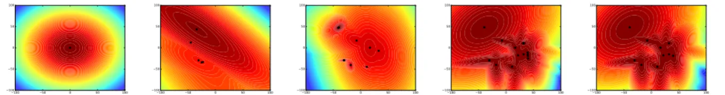
Figure 1: We start with an initial isotropic Gaussian distribution (left) and iteratively improve the approximation and add additional components in order to approximate the desired distribution (right). The three plots in the middle visualize the approximation directly after adding the fifth, tenth and twentieth component.
of the variational distribution. Such approach requires the computation of the Hessian of the objective which is only tractable for mean-field approximations of single Gaussian distributions. In contrast, we use the trust regions directly on the change of the distributions instead of the change of the parameters of the distribution. The information geomet-ric trust regions in this paper allow for efficient estimation of GMMs with full covariance matrices without requiring gradient information fromp∗.
Black-box Variational Inference methods do not make strong assumptions on the model family (Salimans & Knowles,2013;Ranganath et al.,2014) and can therefore also be used for learning GMM approximations. Salimans & Knowles(2013) derive a fixed point update of the natural parameters of a distribution from the exponential family that corresponds to a Monte-Carlo estimate of the gradient of Eq. (1) preconditioned by the inverse of their empirical covariance. By making structural assumptions on the target distribution, they extend their method to mixture models and show its applicability to bivariate GMMs.Ranganath et al. (2014) also use Monte-Carlo gradient estimates of Eq. (1) and apply Rao-Blackwellization and control variates to re-duce its variance. The work ofWeber et al.(2015) already explored the use of Reinforcement Learning for VI but for-malizing VI as sequential decision problem. However, only simple policy gradient methods have been proposed in this context which are unsuitable for learning GMMs.
Closely related to our work are two recent approaches for Variational Inference that concurrently explored the idea of applying boosting to make the training of GMM approx-imations tractable (Miller et al.,2017;Guo et al.,2016). These methods start by minimizing the ELBO objective for a single component and then successively add and optimize new components and learn an optimal weighting between the previous mixture and the newly added component. How-ever, they do not use information-geometric trust region to efficiently explore the sample space and therefore have problems finding all the modes as well as accurate estimates of the covariance matrices. Non-parametric variational in-ference (NPVI) (Gershman et al.,2012) learns GMMs with uniform weights using a second-order approximation of the
ELBO for efficient gradient updates. However, this method only allows for mean field approximations for the mixture components which is a severe limitation as shown in our comparisons. GMMs are also used byZobay(2014) where an approximation of the GMM entropy is used to make the optimization tractable. The optimization is gradient-based and does not consider exploration of the sample space. It is therefore limited to rather low dimensional problems.
5. Experiments
We evaluate VIPS with respect to efficiency of the opti-mization as well as quality of the learned approximations. For assessing efficiency, we focus on the number of func-tion evaluafunc-tions, but also include a comparison with respect to the wall-clock time. As the ELBO objective is hard to use for comparisons as it depends on the current sample set, we assess the quality of the approximation by compar-ing samples drawn from the learned model with ground-truth samples based on their Maximum Mean Discrepancy (MMD) (Gretton et al.,2012). Please refer to the supple-ment how the MMD and the ground-truth samples are com-puted. Please note that the computation of the ground-truth samples is based on generalized elliptical slice sampling (GESS) (Nishihara et al.,2014) which is in most cases com-putationally very expensive. Due to the huge computational demands, we do not consider GESS as competitor. We compare our method to a variety of state-of-the-art MCMC and VI approaches on unimodal and multimodal problems, namely we compare to Variational Boosting (Miller et al.,2017), Non-Parametric Variational Inference (Gershman et al.,2012), Stein Variational Gradient Descent (Liu & Wang, 2016), Hamiltonian Monte Carlo (Duane et al.,1987), Slice Sampling (Neal,2003), Elliptical Slice Sampling (Murray et al.,2010), Parallel Tempering MCMC (Calderhead,2014) and—indirectly, since it is used for ini-tializing variational boosting—black box variational infer-ence (Salimans & Knowles,2013). However, due to the high computational demands, we do not compare to every method on each experiment but rather select promising can-didates based on the sampling problem or on the preliminary experiments that we had to conduct for hyper-parameter
tun-104 105 106 107 108 function evaluations 10-4 10-3 10-2 10-1 100 MMD vips1 vips40 svgd ess hmc npvi vboost0 vboost5 vboost10
(a) German Credit
104 105 106 107 108 function evaluations 10-4 10-3 10-2 10-1 100 MMD vips1 vips40 ess svgd npvi (b) Breast Cancer
Figure 2: Comparison of VIPS to other VI and MCMC methods for two logistic regression tasks. VIPS consider-ably outperformed all other methods already when using only one mixture component (VIPS1) and could only be slightly improved by the GMM on the breast cancer domain.
ing. For VIPS, we use the same hyper-parameters for all experiments. However, we do not add new components if it would increase the number of components above a certain threshold and evaluate different values for this threshold. We perform three experiments on (essentially) unimodal sampling problems taken from related work. We per-form Bayesian logistic regression on the German Credit andBreast Cancerdatasets (Lichman,2013) as described in (Nishihara et al.,2014) and approximate the posterior of the hierarchical Poisson GLM described in (Miller et al., 2017). We designed two challenging toy tasks for evaluat-ing our approach on multimodal problems: samplevaluat-ing from an unknown twenty-dimensional GMM with full covari-ance matrices and distant modes, and sampling the joint configurations of a ten-dimensional planar robot.
We start the experimental evaluation of VIPS by visualizing the iterative improvements of the GMM approximation for the task of approximating an unknown two-dimensional GMM. Figure1shows the log-probability densities of the learned approximation during the optimization and the target distribution (right). We can see that VIPS gradually adds more components and improves the GMM. The final fit with 20 components closely approximates the target distribution. 5.1. Bayesian Logistic Regression
We perform two experiments for binary classification on theGerman credit andbreast cancer datasets (Lichman, 2013). For theGerman creditdataset twenty-five parameters are learned whereas thebreast cancerdataset is thirty-one dimensional. We standardize both datasets and perform linear logistic regression where we put zero-mean Gaussian priors with variance 100 on all parameters.
On theGerman creditdataset we compare against NPVI, ESS, SVGD, HMC and variational boosting. For variational boosting we examine rank-0, rank-5 and rank-10 approx-imations of the covariance matrices. We also performed
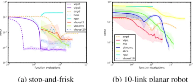
104 105 106 107 function evaluations 10-4 10-3 10-2 10-1 100 MMD vips1 vips5 svgd hmc npvi vboost1 vboost5 vboost10 (a) stop-and-frisk 104 105 106 107 108 function evaluations 10-3 10-2 10-1 100 MMD svgd vips ess ptmcmc slice npvi vboost10
(b) 10-link planar robot
Figure 3: (a) On thestop-and-friskdataset, VIPS1 closely approximates the posterior with roughly 33000 function evaluations. (b) On the 10-link robot experiment VIPS learns a significantly better approximation than competing VI methods and achieves similar sample quality to MCMC.
experiments with full rank approximation but the optimiza-tion always failed after few iteraoptimiza-tions. For our approach we examine two variants, VIPS1 which learns only a single component and VIPS40 which stops adding new compo-nents after forty compocompo-nents. Figure2a shows that the sample quality achieved by VIPS is unmatched by any vari-ational inference method and ESS needs more than two orders of magnitude more function evaluation to achieve a similar MMD to VIPS1. However, we could not measure an advantage of using a GMM instead of single Gaussian dis-tribution on this dataset. As VIPS1 is only learning a single Gaussian, it is also more data-efficient than VIPS40. This result also illustrates the importance of using Gaussian dis-tributions with an accurate estimation of the full covariance as VIPS1 could already outperform competing methods. Figure2bdepicts the achieved MMDs on thebreast cancer dataset. We only compared to the most promising methods from theGerman creditdataset. Although the posterior dis-tribution is unimodal, the GMM variant of our method learns a slightly better approximation than VIPS1, presumably by matching higher order moments of the posterior.
5.2. Multi-level Poisson GLM
We evaluate our method on the problem of learning the pos-terior of a hierarchical Poisson GLM on the 37-dimensional stop-and-friskdataset, where we refer to (Miller et al.,2017) for the description of the hierarchical model. We compared VIPS1 and VIPS5 to HMC, SVGD, variational boosting and non-parametric variational inference. The MMD with respect to the baseline samples is shown in Figure3a. 5.3. Planar Robot
We evaluate our approach on a planar robot with ten de-grees of freedom. We want to sample joint configurations such that the end-effector of the robot is close to a desired position atx= 7andy= 0. The likelihood of a
configu-−2 0 2 4 6 8 10 −4 −2 0 2 4 −2 0 2 4 6 8 10 −4 −2 0 2 4 −2 0 2 4 6 8 10 −4 −2 0 2 4 −2 0 2 4 6 8 10 −4 −2 0 2 4
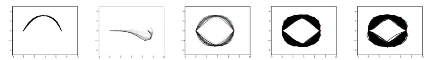
Figure 4: The first three plots visualize typical component means and weights learned by NPVI, VBOOST and VIPS. Components with higher weight are drawn darker. The two rightmost plots show the samples drawn from the VIPS approximation and ground-truth samples, that have been collected during two days on 120 cores using GESS.
104 105 106 107 108 function evaluations 10-4 10-3 10-2 10-1 100 101 MMD svgd vips ess ptmcmc
(a) MMD plotted over iterations
0 5000 10000 15000 20000 time [s] 10-4 10-3 10-2 10-1 100 101 MMD svgd vips (1 core) vips (2 core) vips (4 core) ess ptmcmc
(b) MMD plotted over time
Figure 5: On the GMM experiment, VIPS was able to closely approximate the true mixture model and reliably discovers all ten components. When the number of comput-ing cores is small compared to the components, VIPS can scale almost linearly with the number of cores.
ration is a Gaussian distribution in Cartesian end-effector space with a variance of1e−4in both dimensions. We as-sume a zero mean Gaussian prior in configuration space, where the first joint has variance 1 and the remaining joints have variance 0.04. We compare VIPS40 with ESS, paral-lel tempering MCMC, SVGD, slice sampling, NPVI and VBOOST. The MMD is shown in Figure3b. Figure4 vi-sualizes the learned models of NPVI, VBOOST and VIPS and compares the ground-truth samples with the samples obtained by VIPS. All other VI methods can not represent the complex structure of the modes and get attracted by sin-gle modes resulting in bad approximations. We believe the reason for this behavior is a missing principled treatment of the exploration-exploitation trade-off. VIPS achieves a high sample quality that is comparable to MCMC methods in order of magnitude less function evaluations than MCMC. 5.4. Gaussian Mixture Model
We evaluate our method on the task of approximating un-known, randomly generated 20-dimensional GMMs com-prising ten components. Each dimensions of the component means is drawn uniformly in the interval[−50,50]. The covariance matrices are given byΣ=A>A+I
20where
each entry of the20×20-dimensional matrix Ais sam-pled from a normal distribution with mean0and variance 20. Note that each component of the target distribution can
have a highly correlated covariance matrix, which is even a problem for the tested MCMC methods. Figure5shows the MMD of VIPS40, SVGD, ESS and parallel tempering MCMC plotted over the number of iterations as well as wall-clock time. VIPS was the only method that could reliable be applied to this task. We also briefly evaluated the scaling of the performance with the number of cores. Although parallel computing is not the focus of this paper, the pos-sibility of performing independent updates of the mixture components suggests that the method can make good use of multi-threading. Figure5bshows that VIPS scales almost linearly with the number of cores at least if their number is small, showing the potential of parallelizing our algorithm.
6. Conclusion
VIPS is motivated by the insight from stochastic search that information-geometric trust regions allow for controlled ex-ploration and stable optimization. We transfered the stochas-tic search method MORE to the field of variational inference and demonstrated that it is significantly more efficient than state-of-the-art approaches of VI for learning mean and full covariance of a multi-variate normal distribution. Based on our variant of MORE, we derived a novel method for learning GMM approximations and demonstrated that it is capable of learning high quality approximations of complex, multimodal distributions with a limited amount of function evaluations. Our method makes little assumptions on the unnormalized density function of the desired distribution and is thereby applicable to non-differentiable problems. However, for higher-dimensional problems (e.g. more than 100 dimensions) fitting quadratic surrogates may require too many samples which could be alleviated by using gradi-ent information for constraining the surrogate. Furthermore, learning diagonal surrogates can be preferable for such prob-lems due to better sample- and computational efficiency. For exploration, we start with an approximation with high entropy and decrease it slowly during optimization which can miss modes that are not discovered in the beginning. Actively sampling unexplored regions would result in an anytime algorithm, capable of further improving the approx-imation in the later stages of optimization.
Acknowledgements
This project has received funding from the European Unions Horizon 2020 research and innovation programme under grant agreement No 645582 (RoMaNS). Calculations for this research were conducted on the Lichtenberg high per-formance computer of the TU Darmstadt.
References
Abdolmaleki, A., Lioutikov, R., Lua, N., Reis, L. P., Peters, J., and Neumann, G. Model-Based Relative Entropy Stochastic Search. InAdvances in Neural Information Processing Systems (NIPS), pp. 153–154, 2016.
Abdolmaleki, A., Price, B., Lau, N., Reis, L. P., and Neu-mann, G. Deriving and Improving CMA-ES with Infor-mation Geometric Trust Regions. InThe Genetic and Evolutionary Computation Conference (GECCO 2017), July 2017.
Bishop, C. M.Pattern Recognition and Machine Learning (Information Science and Statistics). Springer-Verlag New York, 2006.
Bishop, C. M., Lawrence, N. D., Jaakkola, T., and Jordan, M. I. Approximating Posterior Distributions in Belief Networks Using Mixtures. InAdvances in Neural Infor-mation Processing Systems, pp. 416–422, 1998.
Blei, D. M., Kucukelbir, A., and McAuliffe, J. D. Variational Inference: A Review for Statisticians. Journal of the American Statistical Association, 2017.
Calderhead, B. A General Construction for Parallelizing Metropolis-Hastings Algorithms.Proceedings of the Na-tional Academy of Sciences of the United States of Amer-ica (PNAS), Nov 2014.
Daniel, C., Neumann, G., and Peters, J. Hierarchical Rela-tive Entropy Policy Search. InInternational Conference on Artificial Intelligence and Statistics (AISTATS), 2012. Deisenroth, M. P., Neumann, G., and Peters, J. A Survey on Policy Search for Robotics.Foundations and Trends in Robotics, pp. 388–403, 2013.
Duane, S., Kennedy, A. D., Pendleton, B. J., and Roweth, D. Hybrid Monte Carlo. Physics Letters B, 195(2):216–222, 1987.
Fan, K., Wang, Z., Beck, J., Kwok, J. T., and Heller, K. Fast Second-order Stochastic Backpropagation for Varia-tional Inference. InProceedings of the 28th International Conference on Neural Information Processing Systems, NIPS’15, pp. 1387–1395, 2015.
Geman, S. and Geman, D. Stochastic Relaxation, Gibbs Distributions, and the Bayesian Restoration of Images. IEEE Transactions on Pattern Analysis and Machine In-telligence, (6):721–741, 1984.
Gershman, S. J., Hoffman, M. D., and Blei, D. M. Nonpara-metric Variational Inference. InProceedings of the 29th International Conference on Machine Learning, 235–242, 2012.
Gretton, A., Borgwardt, K. M., Rasch, M. J., Sch¨olkopf, B., and Smola, A. A Kernel Two-sample Test. Journal of Machine Learning Research, 13:723–773, March 2012. ISSN 1532-4435.
Guo, F., Wang, X., Fan, K., Broderick, T., and Dunson, D. B. Boosting Variational Inference. arXiv:1611.05559v2 [stat.ML], 2016.
Hastings, W. K. Monte Carlo Sampling Methods using Markov Chains and their Applications. Biometrika, 57 (1):97–109, 1970.
Hoffman, M. D. and Gelman, A. The No-U-Turn Sampler: Adaptively Setting Path Lengths in Hamiltonian Monte Carlo. Journal of Machine Learning Research, 15(1): 1593–1623, 2014.
Jaakkola, T. S. and Jordan, M. I. Improving the Mean Field Approximation via the Use of Mixture Distributions. Learning in Graphical Models, 89:163–174, 1998. Kupcsik, A., Deisenroth, M. P., Peters, J., Loh, A. P.,
Vadakkepat, P., and Neumann, G. Model-Based Con-textual Policy Search for Data-Efficient Generalization of Robot Skills. Artificial Intelligence, December 2017. Lichman, M. UCI machine learning repository, 2013. URL
http://archive.ics.uci.edu/ml.
Liu, Q. and Wang, D. Stein Variational Gradient Descent: A General Purpose Bayesian Inference Algorithm. In Lee, D. D., Sugiyama, M., Luxburg, U. V., Guyon, I., and Garnett, R. (eds.),Advances in Neural Information Pro-cessing Systems 29, pp. 2378–2386. Curran Associates, Inc., 2016.
Miller, A. C., Foti, N. J., D’Amour, A., and Adams, R. P. Variational Boosting: Iteratively Refining Posterior Ap-proximations. InProceedings of the International Con-ference on Machine Learning, 2017.
Murray, I., Adams, R., and MacKay, D. Elliptical Slice Sampling. InProceedings of the Thirteenth International Conference on Artificial Intelligence and Statistics, pp. 541–548, 2010.
Neal, R. M. Sampling from Multimodal Distributions using Tempered Transitions. Statistics and Computing, 6(4): 353–366, Dec 1996.
Neal, R. M. Slice Sampling.The Annals of Statistics, 31(3): 705–767, 06 2003. doi: 10.1214/aos/1056562461. Nishihara, R., Murray, I., and Adams, R. P. Parallel MCMC
with Generalized Elliptical Slice Sampling. Journal of Machine Learning Research, 15(1):2087–2112, January 2014.
Peters, J., Muelling, K., and Altun, Y. Relative Entropy Policy Search. InProceedings of the 24th National Con-ference on Artificial Intelligence (AAAI), 2010.
Peterson, C. and Hartman, E. Explorations of the Mean Field Theory Learning Algorithm. Neural Networks, 2 (6):457–494, 1989.
Ranganath, R., Gerrish, S., and Blei, D. Black Box Varia-tional Inference. Artificial Intelligence and Statistics, pp. 814–822, 2014.
Regier, J., Jordan, M. I., and McAuliffe, J. Fast Black-box Variational Inference through Stochastic Trust-Region Optimization. InAdvances in Neural Information Pro-cessing Systems 30, pp. 2399–2408, 2017.
Roberts, G. O. and Stramer, O. Langevin Diffusions and Metropolis-Hastings Algorithms. Methodology and Com-puting in Applied Probability, 4(4):337–357, 2002. Salimans, T. and Knowles, D. A. Fixed-Form Variational
Posterior Approximation through Stochastic Linear Re-gression.Bayesian Analysis, 8(4):837–882, 2013. Schulman, J., Levine, S., Abbeel, P., Jordan, M. I., and
Moritz, P. Trust Region Policy Optimization. In Pro-ceedings of the International Conference on Machine Learning, 2015.
Sutton, R. and Barto, A. Reinforcement Learning: An Introduction. MIT Press, Boston, MA, 1998.
Weber, T., Heess, N., Eslami, A., Schulman, J., Wingate, D., and Silver, D. Reinforced Variational Inference. In Ad-vances in Neural Information Processing Systems (NIPS) Workshops, 2015.
Zobay, O. Variational Bayesian Inference with Gaussian-Mixture Approximations.Electronic Journal of Statistics, 8(1):355–389, 2014. doi: 10.1214/14-EJS887.