Migration, FDI and the Margins of Trade
I,IIAmandine Aubrya, Maurice Kuglerb, Hillel Rapoportc
a
IRES-Université catholique de Louvain
b
UNDP
c
Center for International Development, Harvard University; Department of Economics, Bar-Ilan University; and EQUIPPE, University of Lille
Abstract
Standard neoclassical trade theory models trade, migration and FDI as substitutes in the sense that factor movements reduce the scope for trade and vice versa. This neglects the potential for migration to favor trade and FDI through a reduction in bilateral transaction costs, as emphasized by recent literature on migration and diaspora networks. This paper investigates the relationships between trade, migration and FDI in a context of firms’ heterogeneity. We first present a model of exports and FDI-sales by heterogeneous firms where a (migration-induced) reduction in the fixed costs of setting up either an export or a production facility abroad results in an increase in trade (under certain conditions), sales and most importantly in the FDI-sales to trade ratio. We then test these predictions in a gravity framework using recent bilateral data on migration, trade and FDI. We find that migration – and especially skilled migration – positively affects trade and FDI (at both the extensive and intensive margins), and more so for the latter, resulting in an increase in the FDI to trade ratio, as predicted by our model.
Keywords: Migration, trade, FDI, firms’ heterogeneity
JEL Classification: F22, O1
IThis paper is part of a project on "Migration, International Capital Flows and Economic Development" based
at the Harvard Center for International Development and funded by the MacArthur Foundation’s Initiative on Global Migration and Human Mobility.
IIWe thank Elhanan Helpman, Yona Rubinstein and Rodrigo Wagner for stimulating discussions and Jeffrey
Frankel for collaboration on the broader project. The paper also benefited from comments by participants at the IVth AFD-World Bank Migration and Development Conference. We are grateful to Xuzhi Liu for remarkable research assistance as well as to Olga Romero and Claudia Ramirez.
1. Introduction
Globalization is characterized by a general increase in international transactions for goods, factors and financial flows, with all these components growing much more rapidly than output. For the 1990s only, the growth rate of international trade has been twice that of world output; even more remarkable is the growth of global FDI flows, which has been triple the growth rate of international trade flows over the period. As a result, between 1990 and 2000, the world export/GDP and FDI/GDP ratio have been multiplied by 1.5 and 3 respectively. International migration is also on the rise, as revealed for example by the fact that the total number of foreign-born individuals residing in OECD countries has increased by 50 percent over the same period, a remarkable figure given the fact that in contrast to the liberalization trend that has characterized trade and FDI, restrictive immigration policies have instead been introduced in most receiving countries with the double objective of decreasing the quantity and increasing the
quality of immigration.1 Standard trade theory treats trade and factor flows, as well as labor and
capital flows, as substitutes in the sense that more of one leads to less of the other. Trade reduces the scope for factor flows as it contributes to factor price equalization and, therefore, lowers the incentives to factor mobility. Similarly, factor movements (beyond the Rybszinski cone) reduce price differentials and, hence, the scope for trade. At the same time, capital is expected to flow to where the type of labor used intensively in production is abundant and, other things equal, workers will supply their labor services where the highest salary can be obtained. Through such mechanisms, migration and FDI are substitute ways to match workers and employers located in
different countries.2
There is a growing literature, however, emphasizing that migrant networks facilitate bilateral economic transactions through their removing of informational and cultural barriers between
host and origin countries.3 This "diaspora externality" has long been recognized in the
socio-1
Only the second of these objectives has been achieved. Indeed, the number of highly-skilled immigrants (foreign-born individuals with tertiary education) living in an OECD member country has increased by 70 pecent between 1990 and 2000, but the number of low-skill migrants has risen too, although at a lower pace (13 percent) Docquier and Marfouk [4].
2
In addition, recent studies suggest that there are FDI spillovers on upstream industries in developing countries (e.g., Kugler [16]). To the extent that such spillovers induce adoption of more skill-intensive technologies, they may magnify the substitution effect between skilled migration and FDI.
3
There is also, of course, a literature on vertical FDI and intra-firm trade in intermediate outputs that can explain instances where FDI causes trade.
Following Munshi [20], most studies have used instrumental variables estimation techniques to identify network effects.
logical literature and, more recently, by economists in the field of international trade.4 In many instances, indeed, trade and migration appear as complements (e.g., Gould [9], Head and Ries [10], Combes et al. [3], Iranzo and Peri [14]). Interestingly, such a complementarity has been shown to prevail mostly for trade in heterogeneous goods, where ethnic networks help overcoming information problems linked to the very nature of the goods exchanged (Rauch and Casella [21], Rauch and Trindade [22]). While these studies provide evidence that migration networks have trade-creating effects, they do not consider specifically highly skilled migrants. An exception is Felbermayr and Jung [6], who use bilateral panel data on trade volumes and migration by education levels and find a significant pro-trade effect of migration: a one-percent increase in the bilateral stock of migrants raises bilateral trade by 0.11 percent. However they do not find significant differences across education groups. In a similar spirit, migration may also facilitate the formation of the types of business links which lead to FDI project deployment in a particular location. Hence, while emigration of workers into a country may mitigate to some extent the incentives for FDI from the host to the origin country of migrants, their sheer presence in the host country can be a catalyst to establish the required links to achieve efficient distribution, procurement, transportation and satisfaction of regulations. An important barrier to a multina-tional corporation’s viability to set up a subsidiary in a developing country can be uncertainty, especially the type of uncertainty linked to low institutional quality in candidate host countries
of FDI.5 To the extent that migrants integrate to the business community, a network can emerge
whereby migrants liaise between potential investors and partners (both private and public) in various aspects of setting up a production facility in the country of origin of the migrant. While the channel just described would seem to apply mainly to skilled migrants, there are other chan-nels through which unskilled migrants may also contribute to relax information constraints on FDI. Indeed, participation in the destination country’s labor force reveals information about the characteristics of workers in their home country, thereby reducing uncertainty about the prof-itability of FDI. Hence, both skilled and unskilled migration can, in principle, convey information that will facilitate FDI inflows to the home country. The first studies to explore the links between migration and FDI have focused on sectoral or regional case studies. For example, Aroca and Maloney [2] found a negative correlation between FDI flows and low-skill migration between the border states of Mexico and the United States (i.e., substitutability) while in the spirit of Rauch’s work on trade, Tong [23] finds that ethnic Chinese networks promote FDI between South-East
4
See Docquier and Rapoport [5] for a broader review of the links between skilled emigration and growth in source countries.
5
Asian countries and beyond, especially where the institutional quality is relatively high. The first paper to introduce the “skill" dimension of migration in a bilateral setting is Kugler and Rapoport [17]. Using bilateral FDI and migration data, they investigate the relationship between migration and FDI for U.S./rest of the world flows during the 1990s. The dependent variable is the growth rate of the capital stock of a country (for 55 host countries) that is financed by FDI from the US between 1990 and 2000. This is regressed on the stock of migrants in the US originating from country i in 1990, on the log-difference of the change of that stock between 1990 and 2000, and a number of standard control variables. Regional fixed effects and their interaction with migration are also introduced to deal with potential unobserved heterogeneity. Their results show that manufacturing FDI towards a given country is negatively correlated with current low-skill migration, as trade models would predict, while FDI in both the service and manufacturing sectors is positively correlated with the initial U.S. high-skill immigration stock of that country. Javorcik et al. [15] confirm these results after instrumenting for migration us-ing passeport costs and migration networks with a 30-year lag. Finally, at a micro level, Foley and Kerr [7] quantify firm-level linkages between high-skill migration to the US and US FDI in the sending countries. They combine US firm-level data on FDI and on patenting by ethnicity of the investors and find robust evidence that firms with higher proportions of their patenting activity performed by inventors from a certain ethnicity subsequently increase their FDI to the origin country of the inventors. They use ethnicity-year fixed effects to control for unobserved heterogeneity, and also instrument the ethnic workforce share in each firm using city-level data on invention growth by ethnicity. They find that a one percent increase in the extent to which a firm’s pool of inventors is comprised of a certain ethnicity is associated with a 0.1 percent increase in the share of affiliate activity conducted in the country of origin of that ethnicity. This provides firm-level evidence of a complementary relationship between high-skill immigration and multinational firms’ activity.
However, to the best of our knowledge, this paper is the first to investigate the relationships between trade, migration and FDI in a unified framework, and to do so while acknowledging the role of firms’ heterogeneity (Melitz [19]) in determining the margins of trade. In section 2, we provide a theoretical background of exports and FDI by heterogeneous firms where a (migration-induced) reduction in the fixed costs of setting up either an export or a production facility abroad results in an increase in FDI and, most importantly, in the FDI to export sales ratio. Such framework allows us to better identify the impact of the "diaspora externality" on the firm’s decision between exports and FDI. A consequence is the opportunity to better source and then alleviate potential endogeneity issues that the literature faces when analyzing the relation
between FDI and migration. Indeed, following Helpman et al. [12]’s method, we derive the effect of migration on the extensive margin from a firm level decision. This firm’s choice following the (migration-induced) reduction in the fixed cost seems less likely having been driven by the past aggregate FDI-sales. Moreover, by taking the relative sales, we focus on the relationship between the migration and proximity-concentration tradeoff. This narrower relation should re-duce the endogeneity issue because the potential omitted variable bias could only exist if any unobserved shock is correlated with migration and the relative minimization cost determining the relative sales. We then test these predictions in a gravity framework using recent bilateral data on migration, trade and FDI. Section 3, 4 and 5 respectively describes the data used, the empirical methodology and the results. We find that migration - and especially skilled migration – positively affects trade and FDI (at both the extensive and intensive margins), and more so for the latter, resulting in an increase in the FDI to trade ratio, as predicted by our model. Section 6 concludes.
2. Theoretical framework
The model builds on Helpman et al. [13] (henceforth HMY) and Helpman et al. [12] (henceforth HMR), from whom we borrow the notations.
2.1. Basic setup
Consider a world with J countries, indexed by j=1,2,. . . ,J. Each country is assumed to consume and produce a continuum of goods indexed by l. Country j’s utility function is given by:
ui = Z i∈Bi xαj(l)dl 1 α (1)
where Bi is the set of products available for consumption in country j. xj(l) is country j’s
consumption of product l. The parameter 0 <α< 1 determines the elasticity of substitution
across products, which is =1−α1 >1. This elasticity is the same in every country. Let Yj be the
income of country j, which is equal to its expenditure level. Then country j’s demand for product l is:
xj(l) =
pj(l)−
wherepj(j) is the price of product l in country j andPj is country j’s ideal price index, given by: Pj = Z l∈Bj pj(l)1−dl !(1−1) (3)
It uses a units of bundles to produce one unit of the differentiated good. The cost of one unit of
bundle is cj in country j. Each firm uses an expenditure-minimizing combination of inputs that
costs cja. We suppose that every country has the same distribution of a, therefore a is only a
measure of comparative productivity across firms within the same country. cj is country specific,
reflecting differences in factor prices across countries. Therefore, every firm in country j draws its productivity from the distribution G(a). Note that since a is the unit cost, 1/a is a measure of the firm’s productivity level.
Some of the products are produced domestically, where others are produced in foreign countries. Each firm produces a distinct good, and firms in different countries produce different goods.
Sup-pose country j hasNj firms, then the total number of differentiated product is given byPJj=1Nj.
Finally, we assume there are two additional costs per foreign market associated with exporting:
a fixed cost cjfij of getting the exporting permission and build up the sales network, and a
melting iceberg transportation cost τij. Here we choose to express the fixed cost in units of
cj. This choice is arbitrary but it does not affect the results since any other differences could
be subsumed by the coefficient fij. If the firm chooses to serve foreign markets in the form of
horizontal FDI, it does not bear transportation costs but will produce in the foreign country and
face the marginal production cost ci (the productivity of the firm remains the same). Beyond
the building up and the sales network costcjfij, the firm must bear an additional cost of setting
up foreign subsidiaries cjgij. Therefore the total fixed cost of FDI is given by cj(fij+gij).
The difference between the two fixed costs measures then the plant level returns to scale. Those additional costs to serve a foreign market explain how a firm chooses the channel through which it sells products abroad. This choice is driven by the proximity-concentration tradeoff.
There is monopolistic competition in final products. The price charged to maximize profits by
each firm is cja
α in domestic market,
τijcja
α in the foreign market in case of exports, and
cia
α in
2.2. Determination of bilateral trade and FDI activities
The profit from serving the domestic market is given by:
(1−α) cja αPj 1− Yj >0, (4)
meaning that it is profitable for all the existing firms to serve the domestic market. In addition, firms can also serve the foreign market, with the profit from exporting being given by:
(1−α) τijcja αPi 1− Yi−cjfij, (5)
Sales in country i6=j are only profitable if a≤aij, whereaijis defined as the required productivity
threshold for exporting (i.e. πpij (aij) = 0):
axij = (1−α)Yi cjfij 1 −1 αPi τijcj . (6)
Alternatively, firms can serve the foreign market by building up a production subsidiary abroad, which would yield the following profits:
(1−α) cia αPi 1− Yi−cj(fij+gij), (7)
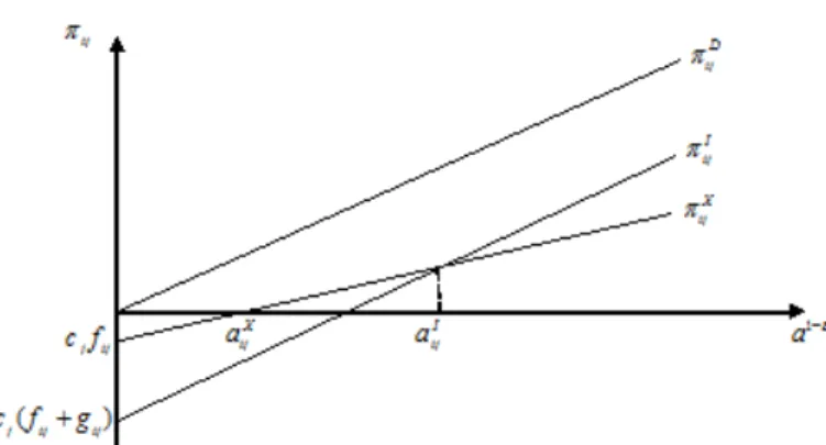
As Figure 1 shows, the productivity threshold required for FDI to be profitable is defined such
that πXij=πIij: aIij = (1−α)Yi cjgij −11 αPi τijcj (τijcj ci )−1−1 −11 . (8)
Implicitly this requires (τijcj
ci )
−1>1, that is, τ
ijcj>ci . Intuitively, in order to make FDI more
profitable than trade, the variable cost of producing in the foreign country must be lower than
that of trade, given the higher fixed costs associated with FDI over trade. Ensuring thataXij>aIij,
that is, the most productive firms engage in FDI, the less productive firms engage in exporting, and the least productive firms only serve domestic market (which is in line with reality - see for example the empirical evidence in HMY) requires that:
aXij aI ij = (1−α)Y i cjfij −11 αPi τijcj (1−α)Y i cjgij −11 αPi τijcj (τijcj ci ) −1−1 1 −1 = g ij fij −11 (τijcj ci ) −1−1 1 −1 >1.
This is equivalent to: gij+fij fij > τ ijcj ci −1
>1. The first term is the ratio of fixed costs for FDI and trade. The second term is the ratio of variable cost of trade v. FDI. The first inequality ensures that the threshold for FDI is higher than that for trade. The second inequality ensures that the threshold for FDI is positive. Different patterns of trade/FDI for each country pair
could be observed. If we denote the cumulative distribution function G(a) with support [aL,aH]
to describe the distribution of a across firms and aH > aXij > aIij > aL, the most productive
firms in country j engage in FDI with country i, the less productive firms engage in trade with country i, and the least productive firms only serve their domestic market. Noting that:
πDj = (1−α) c ja αPj 1− Yj πijX = (1−α) τ ijcja αPi 1− Yi−cjfij πijI = (1−α) cia αPi 1− Yi−cj(fij +gij)
and similarly to HMY, we can draw a graph illustrating the relationships between firms’ decisions
and productivity and showing the different productivity thresholds at hand.6
Figure 1: Exports v. FDI for global firms
. 6
2.3. Reduced fixed costs and the ratio of FDI-sales to trade
We now focus on those country pairs that have both positive trade and positive FDI. Suppose the cumulative distribution of productivity G(a) is Pareto distribution with parameter k and
support [aL,aH]. As in Helpman, Melitz and Yeaple (2004) we assume that k > −1to ensure
that both the distribution of productivity draws and the distribution of firms’ sales have finite
variances. Then G(a)=ak−akL
ak H−akL
. The amount of trade from country j to country i is given by:
SijX = Z aXij aI ij τijcja αPi 1− YiNjdG(a) = kYiNj akH −akL τijcj αPi 1−Z aXij aI ij ak−da (9)
The FDI-related sales from country j to country i is given by:
SijI = Z aIij aL cia αPi 1− YiNjdG(a) = kYiNj ak H −akL τijci αPi 1−Z aIij aL ak−da (10)
Finally, the ratio of trade to FDI-sales is:
SX ij SijI = ci τijcj −1 RaXij aI ij ak−da RaIij aL a k−da = ci τijcj −1(aX ij)k−+1−(aIij)k−+1 (aIij)k−+1−(aL)k−+1 (11) where aXij = (1−α)Yi cjfij 1 −1 αPi τijcj , aIij = (1−α)Yi cjgij 1 −1 αPi τijcj (τijcj ci ) −1−1 1 −1 .
A proportional, possibly migration-induced decrease in the fixed costs for setting up subsidiaries (for exports or foreign production) abroad would affect the productivity thresholds required to do either FDI or trade. More precisely:
Proposition 1. A proportional decrease in the fixed costs to set up a foreign subsidiary either for exports or local production will increase the ratio of FDI-sales to exports.
Proof. Noting the fixed cost for trade asfij∗ =
fij
ω(Mij) and the fixed cost for FDI asg
∗ ij =
gij
ω(Mij),
migration that satisfies the following properties: ω(0) = 0 , ω0(.)>0. The new productivity threshold required for exports and FDI are given by:
aXij∗= (1−α)Yi cjfij∗ !−11 αPi τijcj =aXijω 1 −1 =a X ij(1 +β), (12) aIij∗ = (1−α)Yi cjgij∗ !−11 αPi τijcj (τijcj ci )−1−1 1 −1 =aIijω 1 −1 =a I ij(1 +β). (13)
where β ≡ω−11 −1>0. The amount of trade from country j to country i is now given by:
SijX∗ = kYiNj akH−akL τijcj αPi 1−Z aX ∗ ij aI∗ ij ak−da, (14)
and The FDI-related sales from country j to country i is given by:
SijI∗ = kYiNj ak H −akL τijci αPi 1−Z aI ∗ ij aL ak−da, (15)
Finally, the new ratio of trade to FDI-related sales by:
SijX∗ SI∗ ij = ci τijcj −1 (aX ij)k−+1−(aIij)k−+1 (aIij)k−+1−( aL 1+β)k−+1 . (16)
This new ratio differs from the original ratio only in its denominator, and the denominator is
larger than in the original formula given that k > −1 . The ratio of exports to FDI-sales
therefore decreases when fixed-costs decrease by some fraction.
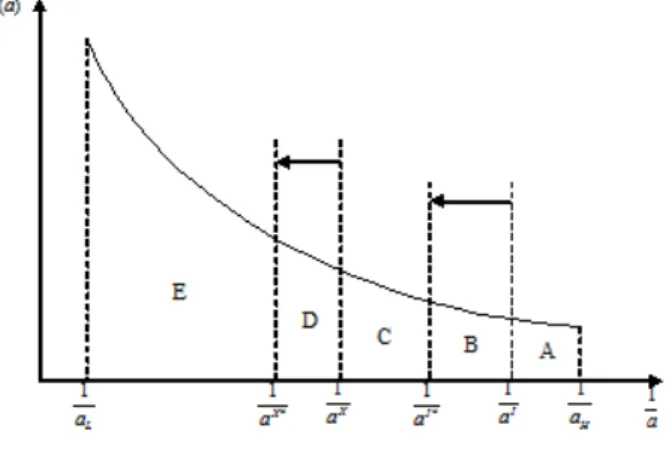
Figure 2 intuitively shows the extent to which this result is driven by the number of firms doing trade and FDI, respectively. Hence, the main testable implication of our model, following from proposition 1, is that the ratio of FDI-sales to exports should increase with migration. However, there is no cross-country bilateral data on the sales of foreign subsidiaries. In our empirical application, therefore, we will use FDI data to proxy for FDI-related sales. In Appendix A, we validate this procedure by showing that for only country for which we have sectoral bilateral data on FDI and FDI-related sales, namely, the United States, there is a clear linear relationship between the two.
7
The x-axis labels the productivity , and the y-axis labels the probability distribution function 1
a. The
Figure 2: The effect of migration on sales:exports v FDI7
As shown on Figure 2 , a proportional decrease in the fixed costs moves the productivity
thresh-olds of both exports a1X and foreign direct investment
1
aI to their new positions and to the left.
Note that a proportional decrease reduces the productivity threshold by the same factor (1+β),
therefore a1I moves more to the left than
1
aX does. Before the decrease, the share of firms doing
FDI is given by the area A and that doing exports by the area B+C. After the decrease, these shares respectively become A+B and C+D. Therefore, the ratio of the number of firms doing FDI v. exports is given by:
Before the decrease: RIX=Area(AreaB)+(AreaA) (C) = BA+C
After the decrease: R∗IX=AreaArea((CA)+)+AreaArea((BD)) = CA++BD
R∗IX-R∗IX=AreaArea((CA)+)+AreaArea((BD))−Area(AreaB)+(AreaA) (C) = A(C(B−D+D)()+B+BBC)
When A(B-D)+BB>0, , the ratio of number of firms in FDI to exports increases as the fixed cost decreases. The model in this section shows this is always verified if the distribution of firms is Pareto. Given our definition of the fixed costs either to export or to setup the subsidiary abroad, both exports and FDI are stimulated due to effect of the migration on the sales network. Moreover, the FDI are fostered by the migrants network due to their impact on the setup production costs. Therefore, an increase in the stock of migrants in the export country increases relatively more the FDI than the exports.
3. Data
We describe in this section our data sources and treatment.
3.1. Trade data
The bilateral trade flows are from the CEPII gravity dataset. It provides a "square" gravity dataset for all world pairs of countries for the period 1948 to 2006. There are 203 "‘country titles" in the dataset over the period 2001-2006. All the countries are identified by their ISO3 code. In the original dataset, data was restricted to observations where trade flows are non-missing. Other trade-related data taken from this dataset including indicators of: using the same currency (or belong to currency union), existence of regional trade agreement (free trade agreement), and sharing common legal system.
We expanded the dataset to cover all the pairs between the 203 countries, and assumed zero trade flows if they were missing. In our analysis, the trade data is calculated by taking the average of six year’s trade flows during 2001 and 2006 . The original data used current dollar as unit, therefore we used the US CPI-US data to deflate it before taking the average. The dataset is available
at http://www.cepii.fr/anglaisgraph/bdd/gravity/col\_regfile09.zip. A description of
the dataset can be found on the CEPII website at http://www.cepii.fr/anglaisgraph/bdd/
gravity.htm 3.2. FDI data
The bilateral FDI position (accumulated FDI) are from the OECD International Direct Invest-ment Statistics. It provides foreign direct investInvest-ment record for inflows from all countries to the OECD countries and outflows from the OECD countries to all countries. These records come from each member country. It is possible that country A keeps a record of inflow from country B, and country B keeps a record of outflow from country A. These two records do not need to be equal. The dataset covers the period from 1990 to 2010. In order to fully utilize the FDI dataset, we combined the inflow and outflow dataset into one dataset. In the cases where both inflow and outflow source data are available, we take the outflow source data in our combined dataset. As a result, our dataset covers all the country pairs with at least one of the two countries belonging to OECD.
In our analysis, the FDI data is calculated by taking the average of six year’s FDI positions during 2001 and 2006. The original data used current US dollar million as unit, therefore we used the US CPI-U data to deflate it before taking the average. For certain countries, the earliest
available data in the series is later than 2001. In these cases we start from the earliest data-available date of the period 2001-2006, and take the average of the following years. For example, Estonia has FDI outflow data only starting from the year 2003. In this case, we took the average of 2003-2006 deflated FDI for Estonia, instead of taking the average of 2001-2006 by assuming zero-value observations in 2001 and 2002. In our study, negative FDI is treated as zero.
The dataset is available at OECD ilibrary http://www.oecd-ilibrary.org. The ratio of FDI
to trade is directly computed by dividing FDI by trade. In the case of zero trade, the ratio data is treated as missing (not included in the regressions except for the probit regression). In our probit analysis, zero ratio is considered equivalent to zero FDI.
3.3. Migration data
We use the Frederic Docquier and Parsons [8] dataset, the last extension of the Docquier and Marfouk [4] dataset, which has been extended to include bilateral data on migration by country of birth, skill category (skilled v. unskilled, the former having college education) and gender for 195 sending/receiving countries in 1990 and 2000. The main additional novelty is that the dataset now captures South-South migration based mainly on observations and occasionally on
estimated data points (for the skill structure). See http://perso.uclouvain.be/frederic.
docquier/filePDF/DMOP-ERF.pdf.
3.4. Other data
The geographic data is from CEPII Distances dataset. There are two datasets: country level file geo_cepii.dta and bilateral file distance_cepii.dta. Bilateral variables from distance_cepii dataset include: indicators of sharing border, sharing official language, history of coloniazing; geographic distance. We take the country-specific "landlocked" entry from the geo_cepii dataset. We assigned "1" to the "landlocked" variable of those country pairs where has at least one of the two countries is considered landlocked.
The dataset is available at http://www.cepii.fr/anglaisgraph/bdd/distances.htm.
The "doing business" data is available athttp://www.doingbusiness.org. In our analysis,
sev-eral different doing business indicators were used as restriction variables for our 2-stage regres-sions. These indicators include: time (days) to start a business, procedures to start a business, and procedures to register for property. We build the indicators from the original doing business dataset by translating them into 0-1 dummy variables. Take the "time (days) to start a business" indicator as an example. we will assign the value "1" to the “time to start a business" indicator of countries pair if the receiving country of FDI (trade) has a value above the median of all the countries.
4. Empirical methodology
The model described in section 2 extends the HMR framework into two dimensions. First, we introduce migration as a determinant of trade flows. Second, we consider the determination of FDI flows in addition to trade flows. It then yields a generalized gravity equation that accounts for the self-selection of firms into export markets and their impact on trade volumes and that can assess how changes in migration induce changes in exports and FDI sales. As described in proposition 1, we postulate that migration from the country where firms are targeting sales reduces the costs of both exporting to that country and the costs of setting up a subsidiary in that country. Then the model predicts that a proportional reduction in the fixed costs of selling abroad and the fixed costs of setting up a subsidiary brought about by migration has the effect of increasing both exports and FDI sales. Furthermore, the model predicts the increase in FDI sales exceeds the increase in exports.
The aim of the analysis is then to estimate the log-linearized version of eq. 14, eq. 15 and eq. 16 that relates the logarithm of expot sales, the logarithm of FDI-related sales and the relative sales to the logarithm of the stock of migrant respectively.
The log-linear form of eq. 14, expressing the export volume from i to j yields the following estimating equation:
sXij =β0+θj+θi−λddij +βmmij+ωij+uij (17)
The LHS is log(exports) abroad. The first term on the RHS is a constant. The second and third
terms are selling country and buying country fixed effects respectively.8 The variablemij is the
logarithm of the stock of migrants from country j to country i reflecting the role of migration from
the buying country to the selling country to reduce the transaction costs for sellers. The termdij
is a generic representation of distance including standard bilateral variables commonly included in gravity equation estimation which affect the volume of firm-level exports, such as geographic distance, common border, colonial ties, common language and same legal system. AS HMR, we
assume that the variable trade costs are stochastic due to i.i.d unmeasured trade frictions uij
which are country pair-specific. Therefore, whiledij captures observable variable trade costs,uij
reflects the non-observables variable trade costs and is such that uij v N(0,σ2u). The variable,
8More precisely,θj=log(N
ωij is a term representing the effect of firm heterogeneity and it corrects the potential omitted
variable bias usually present in the estimation of the standard gravity equation.9
Due to the Pareto asumption, the proportional reductions in both fixed cost of selling abroad and the fixed costs of setting up a subsidiary, migration only affect the volume of firm-level exports and not the decision to export.
The estimating equation for the FDI sales is derived in an identical way10:
sIij =β0+θj+θi−λddij+βmmij +ωijI +uij (18)
This equation is similar to eq. 17 except for ωijI which is defined ash(aaI
L)
k−+1− 1 (1+β)k−+1
i 11 In other words, migration does not only affect the volumes of FDI-sales but also the decision to make FDI instead of exporting. Eq. 18 highlights that even tough the reduction of fixed cost has been proportional, it affects FDI sales and exports differently. It also shows how the HMR estimation must be adjusted to correctly specify the relation between FDI sales and migration.
Finally, the definition of ωijI shows how important it is to control for the fraction of firms that
make FDI sales from j to i in order to consistenly estimate the relation between FDI sales and
migration. We follow HMR to define a latent variableZij which enables us to define the variable
WijI.12 Zij is defined as the following
(1−α)Yi αPiaL ci −1 cjgij 1− c −1 i (τijcj)−1 (19)
Zij represents then the ratio of the variable profit related to FDI-sales for the most
produc-tive firm to the fixed costs to set up a subsidiary in country i time the relaproduc-tive variable cost which reflects the proximity-concentration tradeoff. Note that this latent variable which enables
to estimate the unobserved endogenous variable,Wij, has been derived from a firm-level decision.
Eq. 17 and eq. 18 enables us to compare the impact of migrants on exports and FDI-sales and then analyze which type of fixed costs are more affected by the migration.
9ω
ij=[(aX)k−+1−(aI)k−+1]whereaX andaI are defined in eq. 2.3.
10
Assuming identical assumptions concerning the variables trade costs.
11(1 +β)≡ω−11 −1as defined in section 2.
12
The Pareto assumption as well as the specification of the trade and fixed costs enable us to
structurally estimate eq. 17 and eq. 18 using HMR’s method.13 As HMR, we augment those
equations with the the standard Heckman [11] correction for sample selection, ηij. A consistent
estimate of this term is obtained from the inverse Mills ratio. However, it does not correct for the biases due to underlying unobserved firm heterogeneity. In order to correct both for biases due to trading partner selection and firm heterogeneity, we estimate the equation using nonlinear least squares parametrically, semiparametrically and nonparametrically finding robust effects of migration in reducing barriers to trade and FDI. Such method already captures any selection issue as well as a part of the potential omitted variable bias linked to trade barriers as well described in HMR. Moreover, we believe that this estimation method enables to alleviate several identification issues that the literature traditionally faces when analyzing the relation between either trade and migration or FDI-sales and migration. It will well know that those relations potentially suffers from simultaneity issue as well as potential reverse causality. Indeed, on the one hand, unobserved variables such technological shocks in the exporting country may trigger both FDI from j to i (through a cost reduction) and migration from i to j (through a higher real wage). On the other hand, FDI may foster the migration towards the country j that invests (through training in country j or making aware of new opportunities in this country). Trade can also foster migrations through the decrease of the price index and then the increase in real wage. Those identification issues justify why we wanted to define this relationship between the sales abroad and the migration in a theoretical framework including heterogeneous firms as well as the estimation method described above. First, the theoretical framework defined in section 2 enables us to derive the effect of the migration on the extensive margin (the share of firms setting up subsidiary abroad) from a firm decision level. It seems then unlikely that the firm decision of the most productive firm have been driven by the migrants setting up in the country j due to the past FDI-sales done by country j. Second, the fixed effects already capture unobserved characteristics that may have triggers either trade or FDI and migration simultaneously (such the technological shocks mentionned above). Third, the reverse causality should affect current flows of migration. This potential reverse causality explains why we use a lagged stock of migration. Indeed, current flows of migration counts for a small share of the total stock and are not present in lagged stock of migration. Notwithstanding, we suspect that some potential identification issues might still be present. Any unobserved factor affecting either the fixed cost to export or to start a subsidiary abroad and the stock of migrant would lead to an omitted variable bias
13
which include any common characteristics across the country such cultural proximity. We try to circumvent this problem by estimate the linearized version of eq. 16, the ratio between the exports and the sales induced by FDI:
sxij−sIij =β0+θj+θi−λddij+βmmij +ωijratio+uij (20)
The LHS is the logarithm of the relative sales.The first term on the RHS is a constant. The
second and third terms are selling country ((1−)log(cj)) and buying country ((−1)log(ci)))
fixed effects respectively. The variable mij is the logarithm of the migration from country j
to country i. dij captures observable variable trade costs. The variable ωijratio is the share of
firm setting up subsidiary in country i relative to the share of firms exporting. It is defined
as (aX)k−+1−(aI)k−+1
(1+β)(aI
aL)
k−+1
−1
. It derives from the decision of the marginal firm to either export or to set up subsidiary abroad relative to the choice to set up subsidiary abroad for the most productive firm. The effect of migration on the share of exporters relative to the share of firms investing abroad is then determined by a decision at the firm-level. The aim of taking the ratio is then to define the relation between the migration and the decision for a firm serving abroad to either export or sets up a subsidiary. In other words, we analyze how migration affects the proximity-concentration tradeoff. This narrower relation should reduce the endogeneity issue because the potential omitted variable bias could only exist if any unobserved shock is correlated with migration and the relative minimization cost determining the relative sales. Therefore, the only unmeasured shocks would could question the validity of the estimates are those which affect the decision to migrate and the firm’s decision to either export or investing abroad. Although we believe that the specification of the ratio may reduce the potential endogeneity, we suspect that some omitted variable bias may subsist to the fixed effects, the use of the lag of variables or to the ratio’s specification. As we will discussed in depth in the next section, the results we derived for the variables such legal system or common language can be an indicator that some unobserved cultural characteristics can also affect both the migration and the relative decision to invest abroad. Other types of unobserved factors such as any technological shocks could affect the relative decision to invest abroad and the decision to migrate such technological progress in the communication tools. Such shocks might foster FDI relative to trade as well as improve the network of migrants. Those unmeasured country-pair specific shocks hinders the quality of our estimation and preclude any potential causal interpretation. In the next section, after presenting the general results, we further discuss and present different alternative specifications which have been estimate in order to identify the causal effect of the migration on FDI-sales.
5. Results
We first present results for exports and FDI in the same fashion as in HMR. For each table, the results in column 1 present the first stage probit estimation and column 2 the corresponding Heckman flow equation estimation. The exclusion restriction used when we estimate the exports equation is the number of days to start a business in the importing country from the Doing Business database. The number of days to start a business is related to the fixed costs associated with establishing a distribution network in the importing country. When we estimate the FDI equations, we use the number of procedures to start a business in the host country as the exclusion restriction. This represents the fixed cost of setting up a subsidiary production facility. Column 3 provides a benchmark equation that does not correct for any biases. Column 4 provides the parametric estimation correcting for both selection and firm heterogeneity using nonlinear least squares. Columns 5 relaxes the pareto assumption for G(.). The Pareto distribution does not constraint the baseline specification. Finally, Column 6 and Column 7 relax the joint normality assumption for the unobserved trade costs. Those specifications still yield similar results. Column 8 represents the case where only firm heterogeneity is controlled for and column 9 represents the case in which only selection is corrected.
Our results are similar to the one found by HMR using data from a different time period, namely 2001-2006. We find that exports to foreign locations are explained both by selection patterns whereby trading partners are matched as well as underlying unobserved firm heterogeneity de-termining the extensive and intensive margins of trade volume growth. As in HMR, we find that firm heterogeneity induces more substantial biases in estimating the effects of trade frictions in explaining sales abroad. Our results also highlight the different reactions of trade flows and FDI sales according to the type of costs. Indeed, in table A.2 and table A.6. The distance has a stronger effect on trade flows than on the FDI sales currency union and trade agreements and whether a country is landlocked or not do not significantly affect FDI flows. On the contrary, colonial tie has a much stronger impact on the investment abroad than on the exports. Moreover, we need to use different regulation costs to instrument either the formation of trading relation-ship or the decision to set up a subsidiary abroad. Those results lead us to further investigate factors affecting the costs either to export or to build up a subsidiary such as the migration. We then introduce migration as an explanatory variable. As described in section 4, we use the lagged stock of migrants from the importing country living in the exporting country in 2000 in order to alleviate some potential endogeneity issues. We use both total migration and skilled migration stocks, and find differentiated results as to the elasticity of FDI sales and trade flows.
We find that the elasticity of both exports and FDI with respect to the stock of migrants is higher when we consider skilled migrants as opposed to all migrants. We estimate the elasticity of exports to the country of origin of migrants to be 9.5% when we use the stock of skilled migrants. We estimate the corresponding elasticity of FDI to be 24.3%. This indicates that FDI is more sensitive to migration to the home country of multinational corporations than are exports to migration from the importing to exporting country.
From table A.10, we present the results for the ratio between exports and the FDI is taken. As explained above, we aim to estimate the ratio for two reasons. First of all, it enables us to compare how migration affects the relative sales and then to better identify which type of costs would be more affected by the stock of migration. Second, the ratio aims to identify the source of the potential subsisting omitted variables biases and to mitigate them. This relation estimates how the migration affects the relative sales. Therefore, any potential endogeneity issue would subsist if unobserved shocks are correlated with migration and the relative minimization cost determing the relative sales.
The model described in section 2 predicts that the ratio of FDI sales to export sales will be increasing with migration into the exporting country that is also home base to multinationals. We find indeed that the ratio of FDI to exports is higher, the higher the stock of migrants from the buying country. This effect is more pronounced in the case of skilled migrants. The elasticity of the FDI to exports ratio with respect to skilled migration is 18%. This means that for a given increase in migration from country j to country i there is a propensity for from i to j FDI to grow 18% more than exports from i to j. Indeed, the theory predicts that given a proportional fall due to migration in the fixed costs of selling abroad and the fixed costs of setting up production abroad, there is a larger increase in sales associated with FDI than exports. Concerning, the endogeneity issue, taking the ratio between the trade flows and the FDI enables to restrict the relation between migration and the firm’s decision to either export or build a subsidiary abroad. Moreover, we are able to better identify the source of potential endogeneity. Indeed, some variables such legal system or common language reflect some aspects of the cultural proximity between two countries and can then indicate us whether some cultural characteristics could still affect simultaneously the migration and the relative decision to invest abroad. Tables 2 to 10 show that variables such as common language, colonial tie or same legal system affect trade and FDI. These factors are also likely to affect the stock of migrants from country i to country j. For instance, the same legal system increases the average volume of trade by 39.1 % and the average volume of FDI by 45.1%. It also rises the probability to export by 0.8 % and the probability to build a subsidiary in country i by 8%. When the ratio is taken, this variable does
not affect significantly the relative sales but still interfers wih the decision to either export or set up a subsidiary. In other words, an identical legal system in both countries provides a stronger incentive to firms to invest in the sending country instead of exporting. The ratio seems then to alleviate some of the potential endogeneity issue but might not fully eliminate it since some cultural variables seem to also affect the decision to either export or invest abroad. Therefore, some potential omitted variable biases might subsist to the fixed effects, the lag of variables as well as the ratio. Variables such legal system or common language can be an indicator that some cultural characteristics affect simultaneously the migration and the relative decision to invest abroad. Other types of unobserved shocks such as any technological shocks ( such new communication means) could also affect the relative decision to invest abroad and the migration. Those unmeasured country-pair specific shocks might hinder the quality of our estimation and justify why we are still currently working on this potential identification issue.
6. conclusion
The evidence on globalization suggests that while international trade has risen dramatically in recent decades, the rise in FDI and skilled migration is even more pronounced. It is important to understand the linkages among these various dimensions of globalization. In the current paper we explore the relationship between skilled migration and sales abroad (both export and FDI related). The channel we analyze is the international information transmission of migrants about business opportunities in their country of origin. These business opportunities arise both for exporters and investors. The traditional view from the standard trade literature is that migration and sales abroad are substitutes. In that framework, either workers migrate to satisfy foreign demand or foreign demand is satisfied by sales abroad (merchandise shipments or multinational corporation subsidiary set-up). However, when migration reduces transaction costs associated with sales abroad (through business network formation and information diffusion), migration may complement rather than substitute trade and FDI. In particular, migrants who engage in economic activity in their destination country through their interactions convey information to businesses about sales opportunities (both for exports and FDI) in their country of origin. We find that the elasticity of both exports and FDI with respect to the stock of migrants is higher when we consider skilled migrants as opposed to all migrants. The effect is more pronounced in the case of skilled migrants in the sense that when we use the stock of total migrants, we obtain elasticities that are lower. This is true for all specifications. This suggests that skilled migration is the type of migration that is most relevant for understanding the role of migration in reducing transaction costs from selling abroad. We build a model that augments Helpman
et al. [13] and Helpman et al. [12] by incorporating the possibility that the transaction costs (especially their fixed component) associated with selling and producing abroad are reduced by migration. Our model predicts that the ratio of FDI sales to export sales will be increasing with migration into the exporting country that is also home base to multinationals. Indeed, the theory predicts that given a proportional fall, due to migration, in the fixed costs of selling abroad and the fixed costs of setting up production abroad, there is a larger increase in sales associated with FDI than exports. Empirically, we find indeed that the ratio of FDI to exports is higher, the higher the stock of migrants from the buying country living in the seller country.
We estimate the elasticity of exports to the country of origin of migrants to be 9%, when we
use the stock of skilled migrants. We estimate the corresponding elasticity of FDI to be 25%.
This indicates that FDI is more sensitive to migration to the home country of multinational corporations than are exports to migration from the importing to the exporting country. The
elasticity of the FDI to exports ratio with respect to skilled migration is 18%. This means that
for a given increase in migration from country j to country i there is a propensity for FDI from
i to j to grow 18%more than exports from i to j. The predicted theoretical impact of migration
in stimulating FDI sales exceeds the impact on export sales. Empirically, we find as reported above that indeed the elasticity of FDI with respect to migration from the buying country is larger than that of exports, and that indeed the FDI/exports ratio tends to rise with migration. Our results suggest the importance of migration for the formation of international networks for business information diffusion. Both information about foreign distribution and doing business abroad appears to be transmitted by migrants in their destination country about sales in their country of origin. In particular, even after controlling for origin and destination country fixed effects, as well as bilateral variables measuring geographic and institutional distance, migration is a robust determinant of both exports and FDI from the destination country of the migrants to their origin country. The information channel is consistent with the fact that skilled migration rather than total migration has the stronger link with exports and FDI. As the model predicts, we also find that migration has a stronger impact on FDI than on exports. This makes sense since migrants not only transmit information about distribution which is useful for both exports and FDI sales but also transmit information about setting up of production facility which is useful for the multinational corporations in choosing the location of their subsidiaries. The analysis suggests that to the extent that international transactions are facilitated by the information transmitted by migrants, the impact is stronger on FDI than on trade. This is consistent with the view that setting up a subsidiary in a new country requires much more information than simply shipping merchandise.
[1] Alfaro, L., Kalemli-Ozcan, S., Volosovych, V., May 2008. Why doesn’t capital flow from rich to poor countries? an empirical investigation. The Review of Economics and Statistics 90 (2), 347–368.
[2] Aroca, P., Maloney, W. F., 2005. Migration, trade, and foreign direct investment in mexico. World Bank Economic Review 19 (3), 449–472.
[3] Combes, P.-P., Lafourcade, M., Mayer, T., May 2005. The trade-creating effects of business and social networks: evidence from france. Journal of International Economics 66 (1), 1–29. [4] Docquier, F., Marfouk, A., 2006. International migration by educational attainment (1990-2000). In: C. Ozden and M. Schiff (eds). International Migration, Remittances and Devel-opment. Palgrave Macmillan: New York.
[5] Docquier, F., Rapoport, H., September 2012. Globalization, brain drain, and development. Journal of Economic Literature 50 (3), 681–730.
[6] Felbermayr, G. J., Jung, B., August 2009. The pro-trade effect of the brain drain: Sorting out confounding factors. Economics Letters 104 (2), 72–75.
[7] Foley, C. F., Kerr, W. R., 2012. Us ethnic scientists and foreign direct investment placement. Management Science.
[8] Frederic Docquier, Abdeslam Marfouk, C. O., Parsons, C., 2012. Geographic, gender and skill structure of international migration. Working paper, Université catholique de Louvain. [9] Gould, D. M., May 1994. Immigrant links to the home country: Empirical implications for
u.s. bilateral trade flows. The Review of Economics and Statistics 76 (2), 302–16.
[10] Head, K., Ries, J., February 1998. Immigration and trade creation: Econometric evidence from canada. Canadian Journal of Economics 31 (1), 47–62.
[11] Heckman, J. J., January 1979. Sample selection bias as a specification error. Econometrica 47 (1), 153–61.
[12] Helpman, E., Melitz, M., Rubinstein, Y., 05 2008. Estimating trade flows: Trading partners and trading volumes. The Quarterly Journal of Economics 123 (2), 441–487.
[13] Helpman, E., Melitz, M. J., Yeaple, S. R., March 2004. Export versus fdi with heterogeneous firms. American Economic Review 94 (1), 300–316.
[14] Iranzo, S., Peri, G., September 2009. Migration and trade: Theory with an application to the eastern-western european integration. Journal of International Economics 79 (1), 1–19.
[15] Javorcik, B. S., ï¿12zden, a., Spatareanu, M., Neagu, C., March 2011. Migrant networks and
foreign direct investment. Journal of Development Economics 94 (2), 231–241.
[16] Kugler, M., August 2006. Spillovers from foreign direct investment: Within or between industries? Journal of Development Economics 80 (2), 444–477.
[17] Kugler, M., Rapoport, H., February 2007. International labor and capital flows: Comple-ments or substitutes? Economics Letters 94 (2), 155–162.
[18] Lucas, Robert E, J., May 1990. Why doesn’t capital flow from rich to poor countries? American Economic Review 80 (2), 92–96.
[19] Melitz, M. J., November 2003. The impact of trade on intra-industry reallocations and aggregate industry productivity. Econometrica 71 (6), 1695–1725.
[20] Munshi, K., May 2003. Networks in the modern economy: Mexican migrants in the u.s. labor market. The Quarterly Journal of Economics 118 (2), 549–599.
[21] Rauch, J. E., Casella, A., January 2003. Overcoming informational barriers to international resource allocation: Prices and ties. Economic Journal 113 (484), 21–42.
[22] Rauch, J. E., Trindade, V., February 2002. Ethnic chinese networks in international trade. The Review of Economics and Statistics 84 (1), 116–130.
[23] Tong, S. Y., November 2005. Ethnic networks in fdi and the impact of institutional devel-opment. Review of Development Economics 9 (4), 563–580.
Appendix A. FDI data as a proxy for FDI-related sales
As is shown in section 2, proposition 1, a proportional decrease in the fixed costs to set up a foreign subsidiary either for exports or local production will increase the ratio of FDI-related sales to exports. In order to testify the proposition, we need to gather data on FDI-related sales. Unfortunately, in most instances, data on FDI-related sales is not available. In this appendix, we attempt to overcome this data constraint by empirically approximating FDI-related sales with FDI data. We used the US sample, which is the only available source for FDI- sales related data. Figure A.3 depicts the relationship between the amount of US FDI and the foreign affiliate sales in 147 countries worldwide. Countries with missing data on FDI or affiliate sales were excluded from this graph. FDI refers to the year and FDI position, taking the average of 2001-2006 after deflating by the US CPI_U index. Sales refers to the sales of all foreign affiliates. A “foreign affiliate" is a foreign business enterprise in which there is U.S. direct investment, that is, in which a U.S. person owns or controls 10 percent of the voting securities or the equivalent. Here FDI data comes from the CEPII dataset, in line with other sections of this paper.
Figure A.3: US FDI and US foreign affiliate sales, average of 2001-2006
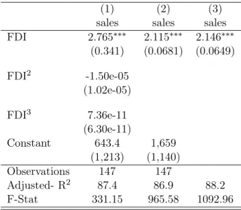
The correlation between the two is 0.9354, indicating a very high linear relationship. Regressing foreign affiliate sales data on FDI with various specifications yields the following result:
Specification (1) includes both higher order products of FDI and constant term. Specification (2) includes only FDI and constant term. Specification (3) includes only FDI and suppresses the constant term. As we can see, adding higher order products does not help increase the
Table A.1: Regression of foreign affiliate sales on FDI
(1) (2) (3)
sales sales sales
FDI 2.765∗∗∗ 2.115∗∗∗ 2.146∗∗∗ (0.341) (0.0681) (0.0649) FDI2 -1.50e-05 (1.02e-05) FDI3 7.36e-11 (6.30e-11) Constant 643.4 1,659 (1,213) (1,140) Observations 147 147 Adjusted- R2 87.4 86.9 88.2 F-Stat 331.15 965.58 1092.96
Standard errors in parentheses
∗
p<0.1,∗∗ p<0.05,∗∗∗ p<0.01
explaining power of FDI on FDI-sales. The coefficient on FDIˆ2, FDIˆ3 and the constant term
are not significant. After suppressing the higher order terms, the adjusted R-squared decreases a little bit, but the overall significance of the model increases substantially as the F-stat tripled. The significance of coefficient on FDI also increases. The constant term is again not significant. This suggests us to try specification (3). This specification yields the highest adjusted R-square stats, F-stat, and the significance of coefficient on FDI. The results show that there is a robust linear relationship between US foreign affiliate sales and US FDI. If we assume that this linear relationship also holds for data on other countries, then our analysis in section 2 would hold for the ratio of FDI to trade. This would validate our empirical study in section 4.
T able A.2: 2 001-2006 A v erage T rade, No Migration (1) (2) (3) (4) (5) (6) (7) (8) (9) Ind(trade) ln( trade) ln(trade) ln(trade) ln(trade) ln(trade) ln(trad e) ln(trad e) ln(trade) Probit ol s b enc hmark nls P olynomial bin 50 bin 100 firm heterogeneit y firm selection ln(distance) -0.0521 ∗∗∗ -1.663 ∗∗∗ -1.663 ∗∗∗ -1.052 ∗∗∗ -1.176 ∗∗∗ -1.154 ∗∗∗ -1.144 ∗∗∗ -0.955 ∗∗∗ -1.732 ∗∗∗ (0.0028) (0.031) (0.031) (0.06 3) (0.045) (0.050) (0.050) (0.049) (0 .031) Common b order -0.0182 0.725 ∗∗∗ 0.725 ∗∗∗ 0.859 ∗∗∗ 0.847 ∗∗∗ 0.859 ∗∗∗ 0.844 ∗∗∗ 0.884 ∗∗∗ 0.662 ∗∗∗ (0.0221) (0.132) (0.132) (0.13 9) (0.129) (0.128) (0.128) (0.131) (0 .134) Currency union 0.0221 ∗∗ 0.842 ∗∗∗ 0.842 ∗∗∗ 0.491 ∗∗ 0.516 ∗∗∗ 0.500 ∗∗ 0.502 ∗∗ 0.433 ∗∗ 0.935 ∗∗∗ (0.0059) (0.202) (0.202) (0.19 3) (0.195) (0.196) (0.196) (0.195) (0.205) F ree trade agreemen t 0.0275 ∗∗∗ 0.897 ∗∗∗ 0.897 ∗∗∗ 0.551 ∗∗∗ 0.695 ∗∗∗ 0.675 ∗∗∗ 0.667 ∗∗∗ 0.495 ∗∗∗ 0.881 ∗∗∗ (0.0034) (0.085) (0.085) (0.09 7) (0.081) (0.082) (0.082) (0.083) (0.086) Coun try is landlo ck ed -0.0139 ∗ -0.647 ∗∗∗ -0.647 ∗∗∗ -0.478 ∗∗∗ -0.475 ∗∗∗ -0.477 ∗∗∗ -0.486 ∗∗∗ -0.454 ∗∗∗ -0.673 ∗∗∗ (0.0077) (0.128) (0.128) (0.12 4) (0.126) (0.127) (0.127) (0.127) (0.128) Same legal sytem 0.0075 ∗∗∗ 0.359 ∗∗∗ 0.359 ∗∗∗ 0.262 ∗∗∗ 0.301 ∗∗∗ 0.296 ∗∗∗ 0.298 ∗∗∗ 0.246 ∗∗∗ 0.359 ∗∗∗ (0.0024) (0.046) (0.046) (0.04 6) (0.046) (0.046) (0.046) (0.046) (0.046) Same official language 0. 0237 ∗∗∗ 0.819 ∗∗∗ 0.819 ∗∗∗ 0.431 ∗∗∗ 0.478 ∗∗∗ 0.469 ∗∗∗ 0.463 ∗∗∗ 0.372 ∗∗∗ 0.869 ∗∗∗ (0.025) (0.065) (0.065) (0.074) (0.069) (0. 070) (0.070) (0.069 ) (0.066) Colonial tie -0.2913 ∗∗ 0.541 ∗∗∗ 0.541 ∗∗∗ 1.744 ∗∗∗ 1.451 ∗∗∗ 1.494 ∗∗∗ 1.515 ∗∗∗ 1.932 ∗∗∗ 0.479 ∗∗∗ (0.199) (0.175) (0.175) (0.245) (0.168) (0. 174) (0.173) (0.176 ) (0.182) Time (da ys) to start a bus iness -0.0955 ∗∗∗ 0.036 (0.0253) (1.058) δ 1.126 ∗∗∗ (0.100) z 3.250 ∗∗∗ 1.330 ∗∗∗ (0.527) (0.070) z 2 -0.493 ∗∗∗ (0.159) z 3 0.028 ∗ (0.016) η 0.543 ∗∗∗ 1.810 ∗∗∗ 0.749 ∗∗∗ (0.125) (0.263) (0.118) Observ atio ns 19547 15800 15800 15800 15800 15800 15800 1580 0 15800 R 2 68.7 68 .7 69.3 69.5 69.6 69.7 69.3 68.8 Standard errors in paren theses.They are clustered b y coun try pair. ∗ p < 0.1, ∗∗ p < 0.05, ∗∗∗ p < 0.01
T able A.3: 2001-2006 A v erage T rade, T otal Migration (1) (2) (3) (4) (5) (6) (7) (8) (9) Ind(trade) ln(trade) ln(trade) ln(trade) ln(trade) ln(trade) ln(trade) ln(trade) ln(trade) Probit ols b enc hmark nl s P olynomial bin 50 bi n 100 firm heterogene it y firm selection ln(total migration in 2000) 0.001819 ∗ 0.096 ∗∗∗ 0.096 ∗∗∗ 0.066 ∗∗∗ 0.073 ∗∗∗ 0.072 ∗∗∗ 0.073 ∗∗∗ 0.062 ∗∗∗ 0.092 ∗∗∗ ( 0. 000945) (0.010) (0.010) (0.011) (0.009) (0.010) (0.0 10) (0.010) (0.010) ln(distance) -0.053 ∗∗∗ -1.595 ∗∗∗ -1.595 ∗∗∗ -1.015 ∗∗∗ -1.127 ∗∗∗ -1.089 ∗∗∗ -1.107 ∗∗∗ -0.936 ∗∗∗ -1.656 ∗∗∗ (0.0032) (0.034) (0.03 4) (0.066) (0. 047) (0.051) (0.051) (0.052) (0.035) Common b order -0.026 0. 288 ∗∗ 0.288 ∗∗ 0.539 ∗∗∗ 0.510 ∗∗∗ 0.521 ∗∗∗ 0.512 ∗∗∗ 0.570 ∗∗∗ 0.253 ∗ (0.0256) (0.134) (0.13 4) (0.151) (0. 132) (0.133) (0.133) (0.134) (0.136) Currency union 0.023 ∗∗ 0.802 ∗∗∗ 0.802 ∗∗∗ 0.439 ∗∗ 0.464 ∗∗ 0.451 ∗∗ 0.459 ∗∗ 0.395 ∗∗ 0.889 ∗∗∗ (0.0057) (0.203) (0.20 3) (0.199) (0. 196) (0.196) (0.197) (0.197) (0.205) F ree trade agreemen t 0.0276 ∗∗∗ 0.715 ∗∗∗ 0.715 ∗∗∗ 0.451 ∗∗∗ 0.594 ∗∗∗ 0.565 ∗∗∗ 0.574 ∗∗∗ 0.406 ∗∗∗ 0.707 ∗∗∗ (0.0034) (0.087) (0.08 7) (0.100) (0. 083) (0.083) (0.083) (0.085) (0.088) Coun try is landlo ck ed -0 .0149 ∗∗ -0.643 ∗∗∗ -0.643 ∗∗∗ -0.464 ∗∗∗ -0.457 ∗∗∗ -0.456 ∗∗∗ -0.450 ∗∗∗ -0.444 ∗∗∗ -0.665 ∗∗∗ (0.0079) (0.129) (0.12 9) (0.127) (0. 127) (0.127) (0.127) (0.128) (0.130) Same legal system 0.00806 ∗∗∗ 0.391 ∗∗∗ 0.391 ∗∗∗ 0.303 ∗∗∗ 0.343 ∗∗∗ 0.334 ∗∗∗ 0.333 ∗∗∗ 0.288 ∗∗∗ 0.390 ∗∗∗ (0.0026) (0.048) (0.04 8) (0.048) (0. 048) (0.048) (0.048) (0.048) (0.048) Same official language 0.0253 ∗∗∗ 0.767 ∗∗∗ 0.767 ∗∗∗ 0.384 ∗∗∗ 0.426 ∗∗∗ 0.408 ∗∗∗ 0.420 ∗∗∗ 0.336 ∗∗∗ 0.814 ∗∗∗ (0.0027) (0.069) (0.06 9) (0.079) (0. 073) (0.075) (0.075) (0.074) (0.070) Colonial tie -0.3475 ∗∗∗ 0.263 0.263 1.516 ∗∗∗ 1.201 ∗∗∗ 1.262 ∗∗∗ 1.231 ∗∗∗ 1.695 ∗∗∗ 0.222 (0.2199) (0.165) (0.16 5) (0.259) (0. 164) (0.168) (0.169) (0.172) (0.171) Time (da ys) to start a bu siness -0.0781 ∗∗∗ 1.24 (0.0462) (0.890) δ 1.044 ∗∗∗ (0.103) z 3.199 ∗∗∗ 1.236 ∗∗∗ (0.558) (0.071) z 2 -0.485 ∗∗∗ (0.169) z 3 0.026 (0.017) η 0.486 ∗∗∗ 1.755 ∗∗∗ 0.605 ∗∗∗ (0.131) (0.282) (0.126) Observ atio ns 17898 14447 14447 14447 14447 14447 14447 14447 14447 R 2 66.7 66. 7 67.3 67.6 67.7 67.9 67.2 66.8 Standard errors in paren theses.They are clustered b y coun try pair. ∗ p < 0.1, ∗∗ p < 0.05, ∗∗∗ p < 0.01
T able A.4: 2 001-2006 A v erage T rade, High Skilled Migration (1) (2) (3) (4) (5) (6) (7) (8) (9) Ind(trade) ln( trade) ln(trade) ln(trade) ln(trade) ln(trade) ln(trad e) ln(trad e) ln(trade) Probit ol s b enc hmark nls P olynomial bin 50 bin 100 firm heterogeneit y firm selection ln(high skilled migr ation in 2000) .000826 0. 095 ∗∗∗ 0.095 ∗∗∗ 0.081 ∗∗∗ 0.091 ∗∗∗ 0.090 ∗∗∗ 0.091 ∗∗∗ 0.078 ∗∗∗ 0.086 ∗∗∗ (0.002) (0.012) (0.012) (0.014) (0.012) (0. 012) (0.012) (0.012 ) (0.012) ln(distance) -0.054 ∗∗∗ -1.620 ∗∗∗ -1.620 ∗∗∗ -0.987 ∗∗∗ -1.106 ∗∗∗ -1.064 ∗∗∗ -1.052 ∗∗∗ -0.927 ∗∗∗ -1.682 ∗∗∗ (0.0033) (0.034) (0.034) (0.06 7) (0.049) (0.054) (0.053) (0.053) (0 .035) Common b order -0.015 0.485 ∗∗∗ 0.485 ∗∗∗ 0.629 ∗∗∗ 0.613 ∗∗∗ 0.631 ∗∗∗ 0.631 ∗∗∗ 0.639 ∗∗∗ 0.455 ∗∗∗ (0.207) (0.135) (0.135) (0.146) (0.132) (0. 132) (0.132) (0.134 ) (0.136) Currency union 0.0237 ∗∗ 0.909 ∗∗∗ 0.909 ∗∗∗ 0.508 ∗∗ 0.540 ∗∗∗ 0.513 ∗∗∗ 0.495 ∗∗ 0.477 ∗∗ 0.988 ∗∗∗ (0.006) (0.204) (0.204) (0.199) (0.197) (0. 197) (0.197) (0.198 ) (0.206) F ree trade agreemen t 0.0287 ∗∗∗ 0.805 ∗∗∗ 0.805 ∗∗∗ 0.485 ∗∗∗ 0.635 ∗∗∗ 0.605 ∗∗∗ 0.600 ∗∗∗ 0.442 ∗∗∗ 0.799 ∗∗∗ (0.006) (0.086) (0.086) (0.100) (0.082) (0. 083) (0.083) (0.085 ) (0.087) Coun try is landlo ck ed -0.0145 ∗∗ -0.637 ∗∗∗ -0.637 ∗∗∗ -0.450 ∗∗∗ -0.444 ∗∗∗ -0.446 ∗∗∗ -0.435 ∗∗∗ -0.436 ∗∗∗ -0.659 ∗∗∗ (0.006) (0.130) (0.130) (0.127) (0.128) (0. 128) (0.128) (0.129 ) (0.130) Same legal system 0.008 ∗∗∗ 0.387 ∗∗∗ 0.387 ∗∗∗ 0.293 ∗∗∗ 0.334 ∗∗∗ 0.326 ∗∗∗ 0.320 ∗∗∗ 0.281 ∗∗∗ 0.388 ∗∗∗ (0.003) (0.048) (0.048) (0.048) (0.048) (0. 048) (0.048) (0.048 ) (0.048) Same official language 0. 0253 ∗∗∗ 0.788 ∗∗∗ 0.788 ∗∗∗ 0.369 ∗∗∗ 0.412 ∗∗∗ 0.397 ∗∗∗ 0.395 ∗∗∗ 0.333 ∗∗∗ 0.838 ∗∗∗ (0.0027) (0.069) (0.069) (0.08 0) (0.074) (0.075) (0.075) (0.075) (0.070) Colonial tie -0.3321 ∗∗ 0.300 ∗ 0.300 ∗ 1.584 ∗∗∗ 1.247 ∗∗∗ 1.319 ∗∗∗ 1.351 ∗∗∗ 1.728 ∗∗∗ 0.273 (0.2165) (0.174) (0.174) (0.25 9) (0.171) (0.175) (0.175) (0.177) (0.179) Time (da ys) to start a bus iness -0.078 ∗∗∗ 0.042 (0.0423) (0.892) δ 1.111 ∗∗∗ (0.103) z 3.292 ∗∗∗ 1.271 ∗∗∗ (0.560) (0.071) z 2 -0.497 ∗∗∗ (0.170) z 3 0.027 (0.017) η 0.416 ∗∗∗ 1.728 ∗∗∗ 0.599 ∗∗∗ (0.132) (0.282) (0.127) Observ atio ns 17898 14447 14447 14447 14447 14447 14447 1444 7 14447 R 2 66.6 66 .6 67.2 67.5 67.7 67.8 67.2 66.7 Standard errors in paren theses.They are clustered b y coun try pair. ∗ p < 0.1, ∗∗ p < 0.05, ∗∗∗ p < 0.01
T able A.5: 20 01-2006 A v erage T rade, Lo w Skilled Migration (1) (2) (3 ) (4) (5) (6) (7) (8) (9) Ind(trade) ln (trade) ln(trade) ln(trade) ln(trade) ln(trade) ln(trad e) ln(tra de) ln(trade) Probit ols b enc hmark nls P olynomial bin 50 bin 100 firm heterogeneit y firm selection ln(lo w skilled migration in 2000) 0.0015 0.096 ∗∗∗ 0.096 ∗∗∗ 0.070 ∗∗∗ 0.075 ∗∗∗ 0.075 ∗∗∗ 0.074 ∗∗∗ 0.066 ∗∗∗ 0.093 ∗∗∗ (0.0009) (0.010) (0.010) (0.0 11) (0.010) (0.010) (0.010) (0.010) (0.010) ln(distance) -0.0532 ∗∗∗ -1.598 ∗∗∗ -1.598 ∗∗∗ -1.014 ∗∗∗ -1.128 ∗∗∗ -1.108 ∗∗∗ -1.106 ∗∗∗ -0.934 ∗∗∗ -1.659 ∗∗∗ (0.0032) (0.034) (0.034) (0.0 66) (0.048) (0.052) (0.052) (0.052) (0.035) Common b order -0.024 0.279 ∗∗ 0.279 ∗∗ 0.516 ∗∗∗ 0.490 ∗∗∗ 0.487 ∗∗∗ 0.489 ∗∗∗ 0.546 ∗∗∗ 0.244 ∗ (0.0032) (0.135) (0.135) (0.1 52) (0.133) (0.133) (0.133) (0.135) (0.136) Currency union 0. 0236 ∗∗ 0.803 ∗∗∗ 0.803 ∗∗∗ 0.439 ∗∗ 0.464 ∗∗ 0.468 ∗∗ 0.460 ∗∗ 0.394 ∗∗ 0.892 ∗∗∗ (0.0058) (0.203) (0.203) (0.1 99) (0.197) (0.196) (0.198) (0.197) (0.205) F ree trade agreemen t 0.0278 ∗∗∗ 0.715 ∗∗∗ 0.715 ∗∗∗ 0.446 ∗∗∗ 0.590 ∗∗∗ 0.570 ∗∗∗ 0.571 ∗∗∗ 0.400 ∗∗∗ 0.707 ∗∗∗ (0.0035) (0.087) (0.087) (0.1 00) (0.083) (0.083) (0.084) (0.085) (0.088) Coun try is landlo ck ed -0.0149 ∗∗ -0.641 ∗∗∗ -0.641 ∗∗∗ -0.463 ∗∗∗ -0.456 ∗∗∗ -0.460 ∗∗∗ -0.455 ∗∗∗ -0.443 ∗∗∗ -0.664 ∗∗∗ (0.0079) (0.129) (0.129) (0.1 27) (0.127) (0.127) (0.127) (0.128) (0.130) Same legal system 0.0080 ∗∗∗ 0.392 ∗∗∗ 0.392 ∗∗∗ 0.303 ∗∗∗ 0.344 ∗∗∗ 0.339 ∗∗∗ 0.336 ∗∗∗ 0.288 ∗∗∗ 0.391 ∗∗∗ (0.0026) (0.048) (0.048) (0.0 48) (0.048) (0.048) (0.048) (0.048) (0.048) Same official language 0.0249 ∗∗∗ 0.771 ∗∗∗ 0.771 ∗∗∗ 0.386 ∗∗∗ 0.429 ∗∗∗ 0.424 ∗∗∗ 0.421 ∗∗∗ 0.336 ∗∗∗ 0.819 ∗∗∗ (0.0027) (0.069) (0.069) (0.0 79) (0.073) (0.075) (0.075) (0.074) (0.070) Colonial tie -0.3429 ∗∗∗ 0.270 0.270 1.517 ∗∗∗ 1.203 ∗∗∗ 1.230 ∗∗∗ 1.251 ∗∗∗ 1.697 ∗∗∗ 0.229 (0.2185) (0.165) (0.165) (0.2 59) (0.163) (0.168) (0.169) (0.172) (0.171) Time (da ys) to start a busi ness -0.1633 ∗∗∗ 0.397 (0.463) (0.789) δ 1.048 ∗∗∗ (0.104) z 3.195 ∗∗∗ 1.240 ∗∗∗ (0.559) (0.071) z 2 -0.483 ∗∗∗ (0.169) z 3 0.026 (0.017) η 0.488 ∗∗∗ 1.756 ∗∗∗ 0.614 ∗∗∗ (0.131) (0.282) (0.126) Observ atio ns 17897 1 4446 14446 1444 6 144 46 14 446 14446 14446 14446 R 2 66.7 66 .7 67.3 67.6 67.7 67.8 67.2 66.8 Standard errors in paren theses. They are clustered b y coun try pair ∗ p < 0.1, ∗∗ p < 0.05, ∗∗∗ p < 0.01
T able A.6: A v erage FDI P osition, No Migration (1) (2) (3) (4) (5) (6) (7 ) (8) (9) Ind(FDI) ln(FDI) ln(FDI) ln(FDI) ln (FD I) ln(FDI) ln(FDI) ln(FDI) ln(FDI) Probit ols b enc hmark nls P olynom ial bin 5 0 bin 100 firm heterogeneit y firm select ion ln(distance) -0.1736 ∗∗∗ -1.248 ∗∗∗ -1.248 ∗∗∗ -1.089 ∗∗∗ -1.128 ∗∗∗ -1.157 ∗∗∗ -1.156 ∗∗∗ -0.917 ∗∗∗ -1.337 ∗∗∗ (0.146) (0.100) (0.100) (0.133) (0.119) (0.114) (0 .118) (0.117) (0.104) Common b order 0.218 ∗∗ 0.395 0.395 0.273 0.315 0.374 0.384 0.210 0.370 (0.108) (0.274) (0.274) (0.246) (0.274) (0.277) (0 .279) (0.277) (0.282) Currency union 0.537 ∗∗∗ 0.188 0.188 0.023 0.083 0.083 0.063 -0 .010 0.068 (0.081) (0.213) (0.213) (0.257) (0.216) (0.215) (0. 217) (0.219) (0.219) F ree trade agreemen t 0.2 28 0.261 0 .261 0. 191 0.209 0.275 0.279 0.149 0.266 (0.040) (0.253) (0.253) (0.207) (0.248) (0.249) (0. 250) (0.251) (0.251) Coun try is landlo ck ed -0.173 ∗∗∗ 0.440 0.440 0.624 0.729 0.718 0.748 0.555 0.540 (0.021) (0.458) (0.458) (0.458) (0.461) (0.477) (0. 497) (0.452) (0.459) Same legal system 0.705 ∗∗∗ 0.603 ∗∗∗ 0.603 ∗∗∗ 0.573 ∗∗∗ 0.562 ∗∗∗ 0.572 ∗∗∗ 0.574 ∗∗∗ 0.486 ∗∗∗ 0.699 ∗∗∗ (0.012) (0.117) (0.117) (0.123) (0.121) (0.122) (0. 123) (0.120) (0.119) Same official language 0.222 ∗∗∗ 0.608 ∗∗∗ 0.608 ∗∗∗ 0.515 ∗∗ 0.535 ∗∗ 0.575 ∗∗∗ 0.584 ∗∗∗ 0.465 ∗∗ 0.599 ∗∗∗ (0.036) (0.210) (0.210) (0.222) (0.209) (0.209) (0. 211) (0.211) (0.211) Colonial tie 0.196 ∗∗∗ 1.254 ∗∗∗ 1.254 ∗∗∗ 0.994 ∗∗∗ 1.003 ∗∗∗ 1.038 ∗∗∗ 1.004 ∗∗∗ 0.753 ∗∗∗ 1.395 ∗∗∗ (0.050) (0.206) (0.206) (0.250) (0.233) (0.237) (0. 238) (0.231) (0.211) Pro ce dures to start a business -0.282 ∗∗∗ -0.342 (0.0227) (0.728 ) δ 0.131 ∗∗∗ (0.246) z 4.039 ∗∗∗ 0.605 ∗∗∗ (0.949) (0. 114) z 2 -1.085 ∗∗∗ (0.313) z 3 0.097 ∗∗∗ (0.032) η 0.0.888 ∗∗∗ 1.726 ∗∗∗ 0.522 ∗∗∗ (0.157) (0.338) (0.149 ) Observ ati ons 748 3 2337 2337 2337 233 7 2337 2337 233 7 2337 R 2 75.1 75.1 75.8 75.6 76.3 76.8 7 5.4 75.3 Standard errors in paren theses. They are clustered b y coun try-pair ∗ p < 0.1, ∗∗ p < 0.05, ∗∗∗ p < 0.01