Possibilistic KNN regression using tolerance intervals

Possibilistic KNN regression using tolerance intervals

Mohammad Ghasemi Hamed, Mathieu Serrurier, Nicolas Durand

To cite this version:

Mohammad Ghasemi Hamed, Mathieu Serrurier, Nicolas Durand. Possibilistic KNN regression

using tolerance intervals. IPMU 2012, 14th International Conference on Information Processing

and Management of Uncertainty in Knowledge-Based Systems, Jul 2012, Catania, Italy. 299,

Part III, pp 410-419, 2012,

<

10.1007/978-3-642-31718-7 43

>

.

<

hal-00938763

>

HAL Id: hal-00938763

https://hal-enac.archives-ouvertes.fr/hal-00938763

Submitted on 24 Apr 2014

HAL

is a multi-disciplinary open access

archive for the deposit and dissemination of

sci-entific research documents, whether they are

pub-lished or not.

The documents may come from

teaching and research institutions in France or

abroad, or from public or private research centers.

L’archive ouverte pluridisciplinaire

HAL, est

destin´

ee au d´

epˆ

ot et `

a la diffusion de documents

scientifiques de niveau recherche, publi´

es ou non,

´

emanant des ´

etablissements d’enseignement et de

recherche fran¸cais ou ´

etrangers, des laboratoires

publics ou priv´

es.

Possibilistic KNN regression using tolerance

intervals

IRIT - Universit´e Paul Sabatier

118 route de Narbonne 31062, Toulouse Cedex 9, France

2

ENAC/MAIAA - 7 avenue Edouard Belin 31055 Toulouse, France

Abstract. By employing regression methods minimizing predictive risk, we are usually looking for precise values which tends to their true re-sponse value. However, in some situations, it may be more reasonable to predict intervals rather than precise values. In this paper, we focus to find such intervals for theK-nearest neighbors (KNN) method with precise values for inputs and output. In KNN, the prediction intervals are usually built by considering the local probability distribution of the neighborhood. In situations where we do not dispose of enough data in the neighborhood to obtain statistically significant distributions, we would rather wish to build intervals which takes into account such distri-bution uncertainties. For this latter we suggest to use tolerance intervals to build the maximal specific possibility distribution that bounds each population quantiles of the true distribution (with a fixed confidence level) that might have generated our sample set. Next we propose a new interval regression method based on KNN which take advantage of our possibility distribution in order to choose, for each instance, the value of K which will be a good trade-off between precision and uncertainty due to the limited sample size. Finally we apply our method on an aircraft trajectory prediction problem.

Keywords: Possibilistic regression, tolerance interval,K-nearest neighbors.

1

Introduction

When dealing with regression problems, it may be risky to predict a point which may be illusionary precise. In these cases, predicting an interval that contains the true value with a desired confidence level is more reasonable. In this scope, one can employ different statistical methods to find a response value prediction interval. These intervals can be estimated once for the whole dataset based on residuals. However, the disadvantage of this approach is to assume that predic-tion interval sizes are independent of test instances. On the other hand, local estimation methods, such as KNN regression, can be used to find an interval that is more likely to reflect the instance neighborhood. In order to calculate such local intervals we have to estimate the probability distribution of the neigh-borhood. But, Even if we know the family of the probability distribution, the

estimated local interval does not reflect the uncertainty on the estimated distri-bution which is caused by the limited size of the sample set. The goal of this paper is to find such interval for KNN.

One interpretation of the possibility theory is in term of families of prob-ability distributions [3]. For a given sample set, there exists already different methods for building possibility distribution which encodes the family of proba-bility distribution that may have generated the sample set[1, 11]. The mentioned methods are based on confidence bands. In this paper we suggest to use tolerance intervals to build the maximal specific possibility distribution that bounds each population quantile of the true distribution (with a fixed confidence level) that might have generated our sample set. The obtained possibility distribution will bound each confidence interval independently with a desired confidence level. On the contrary, a possibility distribution encoding confidence band will bound all the confidence intervals simultaneously with a desired confidence level. This is why our proposed possibility distribution has always smallerα-cuts than the other ones and it still guarantee to obtain intervals which contains the true value with a desired confidence level. This is particularly critical in domains imposing some security constraints. We embed this approach into KNN regression in order to obtain statistically significant intervals. We also propose to take into account the tolerance interval calculus while choosing the parameter K. The obtained interval, will be a good trade-off between precision and uncertainty with respect to the sample size.

This paper is structured as follows: we begin with a background on the possi-bility and probabilistic interpretation of the possipossi-bility theory. We will then look at the different possibility distribution inferred from the same sample set. In the fourth section we will see different KNN interval regression algorithm and finally we compare the mentioned approaches on the prediction of aircraft altitude.

2

Possibility theory

Possibility theory, introduced by Zadeh [14, 5], was initially created in order to deal with imprecisions and uncertainties due to incomplete information which may not be handled by a single probability distribution. In the possibility theory, we use a membership functionπto associate a distribution over the universe of discourseΩ. In this paper, we only consider the case ofΩ=R.

Definition 1 A possibility distribution πis a function fromΩ to(R→[0,1]).

Definition 2 The α-cut Aα of a possibility distributionπ(·) is the interval for which all the point located inside have a possibility degree π(x) greater or equal thanα:Aα={x|π(x)≥α, x∈Ω}

The definition of the possibility measureΠ is based on the possibility dis-tributionπsuch asΠ(A) =sup(π(x),∀x∈A). One interpretation of possibility theory is to consider a possibility distribution as a family of probability distri-butions (see [3]). Thus, a possibility distribution πwill represent the family of

the probability distributions Θ for which the measure of each subset of Ω will be bounded by its possibility measures :

Definition 3 A possibility measureΠ is equivalent to the familyΘof probability measures such that

Θ={P|∀A∈Ω, P(A)≤Π(A)}. (1)

In many cases it is desirable to move from the probability framework to the possibility framework. Dubois et al.[6] suggest that when moving from probabil-ity to possibilprobabil-ity framework we should use the “maximum specificprobabil-ity” principle which aims at finding the most informative possibility distribution. The “most specific” possibility distribution for a finite mode probability distribution has the following formula [4] :

π∗(x) =sup(1−P(I_β∗), x∈I_β∗)

where π∗ _{is the “most specific” possibility distribution, I}∗

β is the smallest β

-content interval [4]. Therefore, given f and its transformation π∗ _{we have :}

A∗

1−β =Iβ∗. The equation (1) states that a possibility transformation using [6]

encodes a family of probability distributions for which each quantile is bounded by a possibility α-cut.

Note that for every unimodal symmetric probability density functionf(·), the smallest β-content intervalI_β∗ off is also its inter-quantile by taking lower and upper quantiles respectively at 1−β

2 and 1−

1−β

2 . Thus, the maximum specified

possibility distributionπ∗(·) off(·) can be built just by calculating theβ-content inter-quantileIβ off(·) for all the values ofβ, where β∈[0,1].

3

Inferring possibility distribution from data

Having a sample set drawn from a probability distribution function, one can use different statistical equations in order to express different kinds of uncertainty related to the probability distribution that underlies the sample set. Thus, it can be valuable to take benefit of possibility distributions to encode such uncertain-ties in a more global manner. Given the properuncertain-ties expected, we can describe two different types of possibility distribution : possibility distribution encoding confidence band and possibility transformation encoding tolerance interval. Af-ter a brief description of the first one, we will focus more deeply on the last one which is the most suitable for regression.

In frequentist statistics, a confidence band is an interval defined for each value

x of the random variable X such that for a repeated sampling, the frequency of F(x) located inside the interval [L(x), U(x)] for all the values ofX tends to the confidence coefficient γ. The confidence band of a parametric probability distribution can be constructed using confidence region of parameters of the underlying probability distribution [2]. In this case the confidence band or its maximum specified possibility transformation represents a family of probability

distribution that may has been generated by all the parameters included in the confidence region used to build the confidence band (see Aregui and Denoeux [1] and Masson and Denoeux [11]).

A tolerance interval is an interval which guarantee with a specified confidence level γ, to contain a specified α% proportion of the population. As the sample set grows, confidence intervals downsize towards zero, however, increasing the sample sample size leads the tolerance intervals to converge towards fixed values which are the quantiles. We will call an α tolerance interval(tolerance region) with confidence levelγ, anα-contentγ-coverage tolerance interval we represent it byI_γ,αT . Eachα-content γ-coverage tolerance, by definition contains at least

α% proportion of the true unknown distribution, hence it can be encoded by the (1−α)-cut of a possibility distribution. So for a given γ we represent α -contentγ-coverage tolerance intervals,α∈(0,1) of a sample set by (1−α)-cuts of a possibility distribution which we name asγ-confidence tolerance possibility distribution (γ-CTP distributionπCT P

γ ).

Possibility transformation encoding tolerance interval : normal case

When our sample set comes from a univariate normal distribution, the lower and upper tolerance bounds (XL and XU, respectively) are calculated by the

equation (2) in which ¯X is the sample mean, S the sample standard deviation,

χ2

1−γ,n−1represents the p-value of the chi-square distribution withn−1 degree

of freedom andZ1₋1−α

2 is the critical value of the standard normal distribution

with probability (1−1_−α

2 ) [7]. The boundaries of the α-cutAα = [XL, XU] of

the built possibility distribution is defined as follows:

XL= ¯X−kS, XU = ¯X−kS wherek= v u u t (n−1)(1 + 1 n)Z 2 1−1−α 2 χ2 1−γ,n−1 (2) We obtain the following possibility distributionπCT P

γ :

πCT P_γ (x) = 1−max{α, x∈Aα} whereAα=Iγ,T1−α (3)

For more detail on the different tolerance intervals see [7]. In the figure (3) we represented the 0.95 CTP distribution (πCT P

0_.95 using equation (2)) for different

sample set drawn from the normal distribution (all having (X, S) = (0,1)). The green distribution represents the probability-possibility transformation of

N(0,1). Note that forn≥100 the tolerance interval is approximately the same as the estimated distribution.

Possibility transformation encoding tolerance interval : distribution free case The problem of non-parametric tolerance interval was first treated by Wilks [13]. Wald [12] generalized the method to the multivariate case. The principle for finding a distribution free α-contentγ-coverage tolerance interval or region of continuous random variableX is based on order statistics. For more

information on finding k in (2) values for distribution free tolerance intervals and regions see [13, 12, 7]. Note that when constructing possibility distributions encoding tolerance intervals based on Wilks method which requires finding metrical head and tail order statistics (Wald definition does not have the sym-metry constraint), we obtain possibility distributions which do not guarantee that our α-cuts include the mode and they are not also the smallest possible

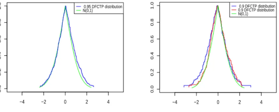
α-cuts. In fact, for any symmetric unimodal distribution, if we choose the Wilks method, we will have tolerance intervals which are also the smallest possible ones and include the mode of the distribution. For the calculation of the sam-ple size requirement for tolerance intervals see [7]. In figure 1, we have the blue curves which represent the distribution-free 0.95-confidence tolerance possibility distribution for a sample set of size 450 (0.95 DFCTP distribution) drawn from

N(0,1) and the green distribution which represent the possibility transformation forN(0,1). In figure (2), we used two different sample set withn= 194 to build two different 0.9 DFCTP distributions. In this example, in order to reduce the required sample size, we restricted the biggestαto 0.98.

● −4 −2 0 2 4 0.0 0.2 0.4 0.6 0.8 1.0 0.95 DFCTP distribution_N(0,1)

Fig. 1. Distribution free 0.95-confidence tolerance possibility distribution for a sam-ple set with size 450 drawn fromN(0,1).

● −4 −2 0 2 4 0.0 0.2 0.4 0.6 0.8 1.0 0.9 DFCTP distribution_{0.9 DFCTP distribution} N(0,1)

Fig. 2.Distribution free 0.9-confidence tol-erance possibility distributions for a sample set with size 194 drawn fromN(0,1).

4

Interval prediction with K-Nearest Neighbors

4.1 K-Nearest Neighbors (KNN)

Smoothing is the process of creating an approximating function that looks for capturing relevant patterns in the data, while filtering noise. In a classical re-gression problem, we havempairs (−→xi, yi) of data where−→xiis a vector of input

variables and yi is the response value. These data follows an unknown mean

functionrwith a random error termǫdefined as:

yi=r(−→xi) +ǫi, where E(ǫi) = 0. (4)

A KNN estimator is a local estimator of the functionrbased on the neighborhood of the considered instance. A KNN is defined as follows :

ˆ r(−→x) = ( n X i=1 Kb(−→x − −→xi))− 1 n X i=1 Kb(−→x − −→xi)yi (5)

whereKb(u) = 21bI(|u| ≤b) (I(·) is the indicator function) is an uniform kernel

with a variable bandwidthb=d(k), where d(k) is the distance between−→x and its furthest K-nearest neighbors. Mack [10] considered the KNN estimator in a general case with kernels other than the uniform kernel. In the same work, he studied the bias and variance of this more general KNN estimator.

4.2 Possibilistic KNN with fixed K

In some problems, we are not only interested in obtaining the most probable regression response value, but we would rather look for intervals which for all input instances simultaneously contain their corresponding response values with a desired probability. It means that the frequency of all the response variables which are contained in their corresponding prediction intervals is at least the prefixed given value. As we saw in the definition of smoothing, equation (4), we suppose that the error is a random variable. Based on our a priori knowledge about the distribution of the error we can use different statistical methods to predict a such intervals.

In machine learning problems, it is common to suppose that the response variable yi in regression is a random variable distributed with N(f(xi), σ2i)

where σ2

i = V ar(ǫi) and estimate yi by its maximum likelihood estimation

ˆ

yi = N( ˆf(xi),σˆ2i). Based on the normality assumption of the errors, there

are two methods used in order to estimate N(f(xi), σi2). In the case of

ho-moscedasticity (the variance of the distribution is constant) for all error terms, the sample variance of the residuals will be used as the estimation of the variance of error. This method is usually used for global approaches like ordinary least square estimation, SVM or neural networks in which the model is assumed to be homoscedastic, or with negligible heteroscedasticity. The heteroscedasticity (the variance depends on the input vector) may also be ignored when we do not dispose of enough data in order to perform significant evaluations. In the other hand, if we assume that our model is heteroscedastick, one can estimate the dis-tribution of the error by a normal disdis-tribution which its mean is still estimated by the KNN estimated value and its variance is estimated by the variance of the sample set in the neighborhood of xi. Since KNN is a local estimation method

used for situations where it is less efficient to use a global model than a local one, exploiting the neighborhood of the input data to estimate the local distribution of error may be justified.

However, if the distribution of the error is estimated locally, it does not take into account the sample size, therefore the estimated quantiles of the error or the response variable may not contain the desired proportion of data. In order to have a more cautious approach, we propose to build a possibility distribution withα-cuts which guarantee to contain, with a confidence levelγ, the (1−α)% proportion of the true unknown distribution. Possibility distributions for the neighborhood of−→xibuilt byγconfidence bands guarantee with confidence level

γ, that all its α-cuts simultaneously contains at least (1−α)% proportion of true unknown distribution that may have generated the neighborhood of −→xi

(the simultaneous condition holds for one input instance). If we consider a γ -CTP distributionπCT P

γ , it guarantee that eachα-cut, independently, will contain

(1−α)% proportion of the true unknown distribution that may have generated the data. Of course, this property is weaker, but it is sufficient in the case of interval prediction and it leads to more specific possibility distributions. Thus, given a input vector −→x we will take the mean ¯X = ˆr(−→x) and the standard deviationSas the standard deviation of theyi of theKnearest instances. After

choosing a value for the confidence level γ (usually 0.95) we build πCT P γ using

Equation 3. Now we will use theπCT P

γ distribution for each instance to obtains

intervals which ensure us to have simultaneously (1−α)% of the response variable for all input instances. It means that for all input vector −→xi the percentage of

α-cuts which contains the correspondingyi will be at leastγ(for ex: 0.95).

4.3 KNN Interval regression with variable K using 0.95 CTP distribution

It is common to fix K and use a weighted KNN estimator, we will call this combination as “KNN regression” or “KNN regression with fixedK”. The fixed

K idea in KNN regression comes from the homoscedasticity assumption. In this section we propose to use the tolerance interval to find the “best”Kfor eachxi.

Let the sample set containing theK-nearest neighbors ofxi beKseti. For each

xi, we begin by a initial value ofK and we build the 0.95 CTP distribution of

Kseti. Now taking theK which yields the most specific 0.95 CTP distribution

means that for each xi, we choose the value of K that has the best trade off

between the precision and the uncertainty to contain the response value. Indeed, whenKdecreases the neighborhood considered is more faithful but uncertainty increases. On the contrary, when K increases, the neighborhood becomes less faithful but the size of the tolerance intervals decrease. In fact the mentioned possibility distribution takes into account the sample size, so its α-cuts will reflect the density of neighborhood. Thus, by choosing theK that minimizes a fixedα-cut (the 0.05-cut in our case) ensures to have the best trade off between the faithfulness of the neighborhood and the uncertainty of the prediction due to the sample size.

The idea is to use prediction intervals which are the most reasonable. For in-stance, for each given−→xiandk, the 0.05-cut of theπγCT P contains at least, with

a prefixedγ confidence level, 95% of the true distribution that may have gener-atedyi, because it contains at least 0.95% of the population of the true unknown

Algorithm 1Possibilistic local KNN

1: M INK←K

2: IntervalSizemin←Inf

3: for all i∈5, . . . , M AXK do

4: Kseti←Find the K nearest neighbors ofxi

5: IntervalSize←0.05-cut of 0.95 CTP distribution ofKseti

6: if IntervalSize≤IntervalSizemin then

7: M INK ←i

8: IntervalSizemin←IntervalSize

9: end if

10: end for

normal distributions that may have generated theKseti. This approach explores

the neighborhood for the value ofkthat is the most statistically significant. The

M INK andM AXK in the algorithm 1 are global limits which stop the search

if we did not found the best K. This may occurs when we have some area of the dataset where the response variable is relatively dense. In practice, we know that this kind of local density is not always a sign of similarity, therefore we put these two bounds to restrict our search in the region where we think to be the most likely to contain the best neighborhood ofxi.

5

Application to aircraft trajectory prediction

In this section, we compare the effectiveness of the regression approaches men-tioned previously with respect to an aircraft prediction problem. Our data set is composed of 8 continuous precise regression variables and one precise response variable. The predictors are selected among more than 30 features obtained by a principal component analysis on a variables set giving informations about the aircraft trajectory, the aircraft type, its last positions and etc. Our goal is to compare these methods when predicting the altitude of a climbing aircraft 10 minutes ahead. Because the trajectory prediction is a critical task, we are in-terested in predicting intervals which contains 95% of the time the real aircraft position, thus we mainly use the inclusion percentage to compare method results. The database contains up to 1500 trajectories and all the results mentioned in the following are computed from a 10-cross validation schema. In a first attempt we will use 2

3of instances will to tune the hyper-parameters. Then all of instances

will serve to validate the results using a 10-cross validation schema. In the hyper-parameters tuning we used the Root Mean Squared Error (RMSE) of response variable (trajectory altitude) to find the best fixedKand localK. The final result for the fixedKwasK= 11 withRM SE= 1197 and (M INK, M AXk) = (7,30)

with RM SE= 1177 for KNN regression with variable K. The kernel function used in our methods was the Tricube kernel Kb(u) = 8170b(1− |u|

3

)3

I{|u|≤b} .

The RMSE found by the two approaches demonstrate that, for this data set, the variableK selection method is as efficient as the conventional fixedK method. We used the following methods to estimate a prediction interval for our response

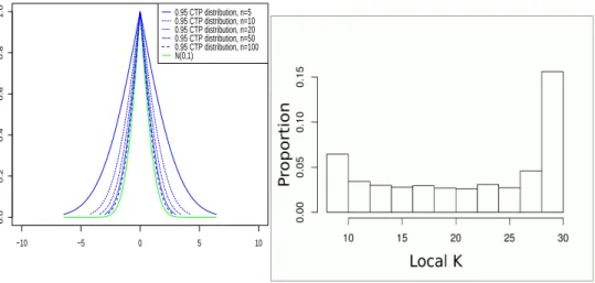
variable : “KNN Interval regression with variable K using 0.95 CTP distribu-tion” (VKNN-CTP), “KNN interval regression using 0.95 CTP distribution” (KNN-CTP), “KNN Interval regression with global normal quantile” (KNN) and “KNN Interval regression with local normal quantile” (LKNN). The table below contains the mean interval size together with their standard deviation in parenthesis and the inclusion percentage of the compared methods. We can notice that the conventional fixedKKNN approaches (KNN-normal global and local) are not enough underestimate the confidence interval size. As expected, the KNN approaches based on the 0.95 CTP distribution, always over estimate these intervals. The most specific estimation is made with the VKNN-CTP al-gorithm. Figure 4 shows the histogram of different values of K found by using the 0.95 CTP distribution. We can observe that the values ofK are uniformly distributed along the range with a maximum reached forK= 25. It suggest, as expected, that the dataset is not homoscedastic.

KNN LKNN KNN-CTP VKNN-CTP Inclusion percentage 0.933 0.93 0.992 0.976 0.95 Interval size (A0.05) 4664 (0) 4694 (1397) 7865 (2341) 5966 (1407)

Table 1.Inclusion percentage compared to the interval size.

● −10 −5 0 5 10 0.0 0.2 0.4 0.6 0.8 1.0 0.95 CTP distribution, n=5 0.95 CTP distribution, n=10 0.95 CTP distribution, n=20 0.95 CTP distribution, n=50 0.95 CTP distribution, n=100 N(0,1)

Fig. 3.0.95-confidence tolerance possibility distributions for a sample set with sizes 5 to 100 and (X, S) = (0,1) in green.

Fig. 4.Histogram ofKfound by using 0.95 CTP distribution.

6

Conclusion

In this work, we propose a method for building a possibility distribution encod-ing tolerance intervals of a sample set drawn from a normal distribution with unknown parameters. Theα-cuts of theπCT P

γ distribution bound the (1−α)%

proportions the true unknown normal distribution with the confidence level γ, regardless of the size of the sample set. Then, we embed these new kind of pos-sibility distributions into a KNN regression algorithm. The suggested method is valuable to be employed for heteroscedastick data. This approach exploits the neighborhood in order to find an “optimal”K for each input instance. The possibility distribution allows us to choose intervals for the prediction that are guaranteed to contain a chosen amount of possible response values. We compared our approach with classical ones on an aircraft trajectory prediction problem. We show that classical KNN provide smaller confidence intervals which fail to guar-antee the required level of inclusion percentage. For future works, we propose to build in the same way the possibility distributions encoding prediction intervals [8][9]. We will also extend this approach to normal mixtures and distribution free sample sets.

References

1. A. Aregui and T. Denœux. Constructing predictive belief functions from continuous sample data using confidence bands. InISIPTA, pages 11–20, July 2007.

2. R. C. H. Cheng and T. C. Iles. Confidence bands for cumulative distribution functions of continuous random variables. Technometrics, 25(1):pp. 77–86, 1983. 3. D. Didier. Possibility theory and statistical reasoning. Compu. Stat. Data An.,

51:47–69, 2006.

4. D. Dubois, L. Foulloy, G. Mauris, and H. Prade. Probability-possibility transfor-mations, triangular fuzzy sets and probabilistic inequalities. Rel. Comp., 2004. 5. D. Dubois and H. Prade. Fuzzy sets and systems - Theory and applications.

Aca-demic press, New York, 1980.

6. D. Dubois, H. Prade, and Sandra Sandri. On possibility/probability transforma-tions. InIFSA, pages 103–112, 1993.

7. G. J. Hahn and W. Q. Meeker. Statistical Intervals: A Guide for Practitioners. John Wiley and Sons, 1991.

8. G.J. Hahn. Factors for calculating two-sided prediction intervals for samples from a normal distribution. JASA, 64(327):pp. 878–888, 1969.

9. H. S. Konijn. Distribution-free and other prediction intervals.Am. Stat., 41(1):pp. 11–15, 1987.

10. Y. P. Mack. Local properties ofk-nn regression estimates. 2(3):311–323, 1981. 11. M. Masson and T. Denoeux. Inferring a possibility distribution from empirical

data. Fuzzy Sets Syst., 157:319–340, February 2006.

12. A. Wald. An extension of wilks’ method for setting tolerance limits.Ann. of Math. Stat., 14(1):pp. 45–55, 1943.

13. S. S. Wilks. Determination of sample sizes for setting tolerance limits. Ann. of Math. Stat., 12(1):pp. 91–96, 1941.

14. L.A. Zadeh. Fuzzy sets as a basis for a theory of possibility. Fuzzy Set. Syst., 1(1):3–28, 1978.