University of Kent
School of Economics Discussion Papers
An empirical validation protocol
for large-scale agent-based models
Sylvian Barde, University of Kent
Sander van der Hoog, Bielefeld University
July 2017
An empirical validation protocol
for large-scale agent-based models
?
Sylvain Barde
aSander van der Hoog
bJuly 4, 2017
Abstract
Despite recent advances in bringing agent-based models (ABMs) to the data, the estimation or calibration of model parameters remains a challenge, especially when it comes to large-scale agent-based macroeconomic models. Most methods, such as the method of simulated moments (MSM), require in-the-loop simulation of new data, which may not be feasible for such computationally heavy simulation models.
The purpose of this paper is to provide a proof-of-concept of a generic empirical validation method-ology for such large-scale simulation models. We introduce an alternative ‘large-scale’ empirical val-idation approach, and apply it to the Eurace@Unibi macroeconomic simulation model (Dawid et al., 2016). This model was selected because it displays strong emergent behaviour and is able to generate a wide variety of nonlinear economic dynamics, including endogenous business- and financial cycles. In addition, it is a computationally heavy simulation model, so it fits our targeted use-case.
The validation protocol consists of three stages. At the first stage we use Nearly-Orthogonal Latin Hypercube sampling (NOLH) in order to generate a set of 513 parameter combinations with good space-filling properties. At the second stage we use the recently developed Markov Information Criterion (MIC) to score the simulated data against empirical data. Finally, at the third stage we use stochastic kriging to construct a surrogate model of the MIC response surface, resulting in an interpolation of the response surface as a function of the parameters. The parameter combinations providing the best fit to the data are then identified as the local minima of the interpolated MIC response surface.
The Model Confidence Set (MCS) procedure of Hansen et al. (2011) is used to restrict the set of model calibrations to those models that cannot be rejected to have equal predictive ability, at a given confidence level. Validation of the surrogate model is carried out by re-running the second stage of the analysis on the so identified optima and cross-checking that the realised MIC scores equal the MIC scores predicted by the surrogate model.
The results we obtain so far look promising as a first proof-of-concept for the empirical validation methodology since we are able to validate the model using empirical data series for 30 OECD countries and the euro area. The internal validation procedure of the surrogate model also suggests that the combination of NOLH sampling, MIC measurement and stochastic kriging yields reliable predictions of the MIC scores for samples not included in the original NOLH sample set. In our opinion, this is a strong indication that the method we propose could provide a viable statistical machine learning technique for the empirical validation of (large-scale) ABMs.
Keywords: Statistical machine learning; surrogate modelling; empirical validation.
?We are grateful to Herbert Dawid, Jakob Grazzini, Matteo Richiardi, and Murat Yıldızo˘glu for helpful discussions and
suggestions. In addition, the paper has benefited from comments by conference participants at CEF 2014 held in Oslo, and CEF 2016 held in Bordeaux. SH acknowledges funding from the European Union’s Horizon 2020 research and innovation programme under grant agreement No. 649186 - Project ISIGrowth (”Innovation-fuelled, Sustainable, Inclusive Growth”).
Non-Technical Summary
Despite recent advances in bringing agent-based models (ABMs) to the data, the estimation or calibration of model parameters remains a challenge, especially when it comes to large-scale agent-based macroeconomic models. Most methods, such as the method of simulated moments (MSM), require in-the-loop simulation of new data, which may not be feasible for models that are computationally heavy to simulate. Nevertheless, because ABMs are becoming an important tool for policy making it is a relevant issue to be able to validate them properly, so that they can be compared to other policy-related models.
Our work proposes a new 3-stage protocol for validating computationally demanding simulation models, based on previous work by Salle & Yildizoglu (2014). The major advantage of this protocol is that it relies on a set of metrologies that are all available as ‘off-the-shelf’ software, requiring only a coordination of their implementation:
1. Efficient sampling & Data generation: The protocol start by generating an efficient sampling of the parameter space of the ABM, using the Near-Orthogonal Latin Hypercube (NOLH) design of Cioppa and Lucas (2007). This is followed by the generation of simulated data using the ABM on the sample points provided by the NOLH. This is the computationally heavy step, which only needs to be performed once.
2. Probabilistic modelling using MIC scoring & Empirical data: The simulated data is first used to train the Markov Information Criterion (MIC) algorithm of Barde (2016a,2016b) on each sample point, which is then scored on the empirical data. This is provides a ‘response surface’ by mapping from the pre-determined set of NOLH parameter calibration points into a fitness landscape using the MIC score as the fitness metric.
3. Surrogate modeling of MIC Response Surface using kriging: In the final stage we use kriging (Krige, 1951) to generate a surrogate model of the set of MIC responses and obtain an interpolated ‘MIC response surface’. By optimizing over this simpler model it is relatively quick to find new candidate sample points with possibly better performance.
The 3-stage protocol is applied to the Eurace@Unibi model of Dawid et al. (2016,2017). This macroeconomic ABM displays strong emergent behaviour and is able to generate a wide variety of nonlinear economic dynamics, including endogenous business and financial cycles. In addition, it is a computationally heavy simulation model, so it fits our targeted use-case. The empirical data used for the analysis consists of monthly data for 3 macroeconomic data (Industrial production, CPI and unemployment rate) from 30 OECD countries and the Eurozone.
Following the first step of the protocol 513 distinct sample points are generated using an NOLH design for 8 core parameters of the model. The simulated data generated in the first stage consists of 1000 simulated series of 1000 time periods for each sample point. Because a single series requires 13 minutes and 20 seconds to run, generating the full set requires 114,000 CPU hours. While using a High Performance Computing (HPC) cluster speeds up the process, Eurace@unibi remains a heavy model to simulate. By contrast, the scoring of the data using the MIC in the second stage only requires a modest 513 CPU hours.
The results obtained by applying the protocol to the Eurace@unibi model are promising, as tight estimated are obtained for several parameters of the Eurace@unibi. The quality of the kriging model is tested by re-running the protocol on a new sample of points obtained through the optimistion of the response surface, and by verifying that the predicted MIC values provided by the kriging model match the realised MIC score obtained through the validation exercise. The very high correlation (0.926) between the MIC scores predicted by the kriging model and the ones obtained by re-running the entire protocol confirms that kriging provides an accurate interpolation of the MIC response surface.
While this exercise provides a successful proof-of-concept for the protocol, particularly the kriging stage, several weaknesses are identified. A first is the fact that the NOLH design cannot be extended easily if further samples are required. This can be remedied by using another design, such as a sobol sequence, which can be extended more easily. Another weakness is the fact that the MIC measurement relies on univariate conditioning, which probably introduces measurement errors when used in a multivariate setting and reduces the accuracy of the response surface. Solving this problem requires using a multivariate version of the MIC, which is the focus of ongoing research.
1
Introduction
Despite recent advances in bringing agent-based models (ABMs) to the data, the estimation or cali-bration of model parameters remains a challenge, especially when it comes to large-scale agent-based macroeconomic models. Most methods, such as the method of simulated moments (MSM), require in-the-loop simulation of new data, which may not be feasible for models that are computationally heavy to simulate.1 Nevertheless, ABMs are becoming an important tool for policy making and it is therefore a relevant issue to be able to compare ABMs to other policy-related models:
“With regard to policy analysis with structural macroeconomic models, an important question is how agent-based models can be used to deliver answers to the type of questions policy makers typically ask of DSGE models. [...] A comparison of agent-based and DSGE models with regard to such questions should be tremendously useful for practical macroeconomic policy analysis.” (Wieland et al., 2012, p.12).
Currently two main challenges exist for agent-based macroeconomists: bringing their models to the data and bringing them to the policy-makers. To address the Lucas Critique (Lucas, 1976) agent-based modellers should generate models that are both empirically validated and policy-relevant. For such empirically and policy-relevant ABMs, the replication of stylized facts does not appear to be a strong enough criterion for model selection since in principle multiple underlying causal structures could generate the same statistical dependencies and therefore match the same set of stylized facts equally well (Guerini and Moneta, 2016). In this view, model comparison and selection should occur at the level of the underlying causal structures, rather than at the level of the statistical dependencies that result from these structures. According to this approach, the objective for policy-relevant ABMs should be to minimize the distance between the causal mechanisms incorporated in the ABM and the causal mechanisms that underlie the real-world data generating process (RW DGP). At this stage, developing more rigorous methods to compare such causal mechanisms is one of the most important open problems in the agent-based modelling community. Resolving this issue will undoubtedly strengthen the reliability, trust and confidence that both academics and policy-makers put in the policy recommendations coming from such models.
An alternative approach is to remain agnostic about the underlying causal structures and instead try to match the conditional probability structures that are embedded in the data. In this view, the appropriate method for model comparison and selection is to minimize the distance between two distributions, namely the distribution of the data resulting from the model and the distribution of the empirical data. This is the approach we have adopted here.
The purpose of this paper is to provide a proof-of-concept of a generic empirical validation methodol-ogy for such large-scale simulation models. We introduce an alternative ‘large-scale’ empirical validation approach, and apply it to the Eurace@Unibi macroeconomic simulation model (Dawid et al., 2016). This model was selected because it displays strong emergent behaviour and is able to generate a wide variety of nonlinear economic dynamics, including endogenous business- and financial cycles. In addition, it is a computationally heavy simulation model, so it fits our targeted use-case.2
Our example application uses a large-scale agent-based macroeconomic model, but in principle the method is agnostic about the underlying DGP. For our method it is irrelevant how the model is imple-mented or how it is simulated, as long as the simulator produces sequential time series data. In addition, the model validation technique that we propose is applicable to any model structure (predictor device) that formally can be represented as a finite-state machine with closed suffix set (FSMX, Rissanen, 1986), or equivalently, by a finite-order Markov process. Most, if not all, computational models in economics can be represented using such formalisms.
In developing our method we rely on the literature on Design and Analysis of Simulation Experiments (DASE, Kleijnen, 2007), which emphasizes the importance of a good Design of Experiments (DoE). This
1A possibility for in-the-loop parameter adjustments would be to use computational steering methods, see Wagner et al.
(2010), who develop an interactive data exploration framework. The parameter adjustments can take place either within-simulation (parameters are adjusted during a within-simulation run), or post-mortem-within-simulation (parameter adjustments occur
is particularly important when dealing with computationally heavy simulation models or data-intensive methodologies, such a laboratory or field experiments, where the experimenter is not able to generate unrestricted amounts of data. In such cases a sequence of carefully designed experiments is required to obtain a sufficient amount of data to cover the range of possible outcomes. In addition, we adopt a Response Surface Methodology (Box and Wilson, 1951), to ensure the validation protocol is able to handle computationally heavy simulation models. Broadly speaking, our proposed methodology consists of three stages, following Salle and Yıldızo˘glu (2014):
1. Start with an experimental design and efficient sampling method, followed by data generation using the simulation model (computationally heavy step).
2. Training and scoring by considering the simulated data as a ‘response surface’ of the model. That is, as a mapping from a pre-determined set of parameter calibration points into a fitness landscape using the MIC score as fitness metric.
3. Surrogate modelling and validation by optimizing over the interpolated ‘MIC response surface’ to find new candidate sample points with possibly better performance.
At the first stage (experimental design, efficient sampling and data generation), we use the Nearly-Orthogonal Latin Hypercube sampling (NOLH) method of (Cioppa, 2002; Cioppa and Lucas, 2007) to generate an efficient experimental design matrix consisting of 513 parameter combinations for eight structural parameters of the Eurace@Unibi model. The resulting sample of the parameter space has two important properties which will be critical for the third stage. Firstly, the sample has good space-filling properties, ensuring good coverage of the parameter space. Secondly, the obtained parameter vectors are nearly orthogonal to each other, increasing the effectiveness of the surrogate model. Once the 513 sample points (parameter calibrations) have been generated by the NOLH sampling method these are used to generate corresponding sets of simulated time series using Monte Carlo simulations of the ABM with 1,000 replication runs per sample.
At the second stage (training and scoring) we use the recently developed Markov Information Criterion (MIC, developed by Barde, 2016a,b) to score the synthetic data sets against the empirical data using macroeconomic target variables for 30 OECD countries and the euro area. The MIC methodology is a generalization of the standard concept of an information criterion to any model that is reducible to a finite-order Markov process. Its main feature of interest is that different models can be scored against an empirical data set using merely the simulated time series data, remaining agnostic about the underlying causal mechanisms and without the need to construct a statistical structure. In order to learn the Markov transition probabilities of the underlying DGP, the Context Tree Weighting algorithm (CTW, developed by Willems et al., 1995) is applied to the simulated time series, yielding the conditional probabilities required to score each model against the empirical data. The CTW algorithm is proven to provide an optimal learning performance, in the sense that it achieves the theoretical lower bound on the learning error. As explained in Barde (2016a), this means that a bound correction procedure can be applied to the raw CTW score to correct the measurement error due to learning, thus enabling an accurate measurement of the informational distance between the model and the data.
By considering the model as an input/output response function, i.e. as a mapping from a space of inputs/parameter calibrations into a space of outputs/variables, we use the MIC score as a fitness measure for each parameter calibration. This concept is then used to construct a ‘model response surface’ that we call the ‘MIC Response Surface’ of the model consisting of the MIC scores for the 513 NOLH sample points. This surface is a fitness landscape over which we interpolate and minimize in the third stage.
At the third stage (surrogate modelling and validation) we use stochastic kriging (Krige, 1951; Klei-jnen, 2017) to construct a surrogate model of the ‘MIC Response Surface’ generated at stage two. The surrogate model is an interpolation between the realized MIC scores yielding predicted MIC scores for model calibrations that have not yet been tried, possibly resulting in new sample points that are promising candidates for better model calibrations with higher fitness/lower MIC scores. We proceed by identifying the local minima across the interpolated MIC Response Surface, selecting those parameter combinations that provide the lowest predicted MIC score, i.e. providing the best fit to the empirical data by mini-mizing the relative Kullback-Leibler distance. Next, validation of the surrogate model is carried out by
generating supplementary training data for the newly identified best parametrisations using the original, computationally heavy, simulation model. After re-running the second stage of the analysis on these supplementary samples and cross-checking the realised MIC values against the predicted MIC scores of the surrogate model, we are able to confirm whether or not the surrogate model is able to detect local MIC minima of the MIC Response Surface. Such an internal validation procedure could be seen as an in-sample prediction test of the surrogate model.3
The results we obtain so far look promising as a first proof-of-concept for the methodology since we are able to validate the model using the empirical data sets for 30 OECD countries and the euro area. The internal validation procedure of the surrogate model also suggests that the combination of NOLH sampling, MIC measurement and stochastic kriging yields reliable predictions of the MIC scores for samples that are outside of the original NOLH sample set. In our opinion, this is a strong indication that the method we propose could provide a viable statistical machine learning technique for the empirical validation of (large-scale) ABMs.
This rest of this paper is organized as follows. In Section 2 we give an overview of related literature. Section 3 provides an overview of our methodology. Section 4 gives a brief overview of the model, the parameters selected for calibration, and the empirical data that we used. Section 5 discusses the results. Section 6 concludes with a discussion of current limitations of the protocol and suggestions for future extensions.
2
Literature
2.1
Key challenges for ABM validation
Ten years ago Windrum et al. (2007) identified several key issues concerning the empirical validation of ABMs in response to a perceived lack of discipline and robustness in the field of agent-based modelling in economics. The first issue is that the neoclassical community has consistently developed a core set of theoretical models and applied these to a wide range of issues. On the other hand, the agent-based community had not yet done so. A second issue is the lack of comparability between different ABMs: “Not only do the models have different theoretical content but they seek to explain strikingly different phenomena. Where they do seek to explain similar phenomena, little or no in-depth research has been undertaken to compare and evaluate their relative explanatory performance.” (ibid., p. 198). Finally, a third issue is the relationship between ABMs and the empirical data: “[E]mpirical validation involves examining the extent to which the output traces generated by a particular model approximate reality.” (ibid.).
Over the course of the last ten years the agent-based modelling community has tackled the first of these important issues successfully, namely to apply the same ABMs to different policy questions and to adopt standard modelling tools. Examples run from agent-based macroeconomic models with deliberately simple structures that focus on a single market transmission mechanism (Arifovic et al., 2013; Assenza and Delli Gatti, 2013; De Grauwe and Macchiarelli, 2015; Riccetti et al., 2015) to models with a more holistic perspective that model a system of integrated markets (Mandel et al., 2010; Dosi et al., 2010; Dawid et al., 2016).4 The field is at a stage where several large-scale, agent-based macroeconomic models have been constructed with the specific purpose of performing macroeconomic policy analyses (see e.g., Dosi et al., 2015; Dawid et al., 2017) and this now necessitates bringing these models to the data.
Progress has been slower, however, on the two issues of model comparison and empirical validation. A key debate, presented below, is to clarify what the goals of empirical validation of ABMs should be. The existing macro-ABMs are all slightly different in scope and in scale, mainly due to their application to different policy domains. This makes a comparison of their predictive accuracy an important aspect that needs to be investigated.5
3Note that the additional training data set produced after the kriging step is minor in relation to the initial data volume
that needs to be generated for the original training data at stage 1. The supplementary data is needed in order to refine the empirical parameter validation at stage 3.
The current paper seeks to address the second and third issues identified above by offering a method-ology for model comparison and model selection against an empirical dataset. This method can be used to bridge the gap between model selection/comparison and model calibration/estimation since it works on the basis of a pre-existing set of parameter calibrations with no new parameter calibrations being generated iteratively (no in-the-loop simulation).
2.2
Validation concepts and methods for ABM
In order to provide some clarity within the wide array of different modelling choices, we classify current models in the Agent-based Macroeconomics literature into two main groups, either small or large-scale agent-based macroeconomic models (see also Richiardi, 2015 and Salle and Yıldızo˘glu, 2014 for similar assessments). Due to the distinct approaches it seems quite difficult to make model comparisons or to do quality assessments, which would explain the lack of a general methodology for model comparison and empirical estimation. The problem gets aggravated due to the lack of objective model selection criteria and quantitative measures of fit to data sets.
A generic model classification scheme for model validation is proposed by Epstein and Axtell (1994), who categorize ABMs into four classes according to their level of empirical relevance:
• Level 0: The model is a caricature of reality, as established through the use of simple graphical devices (e.g., allowing visualization of agent motion).
• Level 1: The model is in qualitative agreement with empirical macro structures, as established by plotting, say, distributional properties of the agent population. (This can be associated to matching stylized facts.)
• Level 2: The model produces quantitative agreement with empirical macrostructures, as established through on-board statistical estimation routines.
• Level 3: The model exhibits quantitative agreement with empirical microstructures, as determined from cross-sectional and longitudinal analysis of the agent population.
The current literature on empirical validation of ABMs shows a progression from models at level-1, concerned with the qualitative matching of stylized facts, to models at level-2, concerned with quantitative estimation. The focus is currently shifting towards the development of more rigorous empirical validation techniques. However, all of the approaches that are currently proposed still use macro variables as the observables. The final step, moving towards models at level-3, would require observables at the micro level. A challenge for such a truly agent-based estimation methodology is data availability at the level of individual agents, which would require highly disaggregated data (see also Chen et al., 2014 and Grazzini and Richiardi, 2014).
Lux and Zwinkels (2017) survey the burgeoning literature on the empirical validation of agent-based models over the last decade. They discuss various methods for estimation and calibration of ABMs, covering reduced-form statistical models, Method of Simulated Moments (MSM), numerical Maximum Likelihood (ML) including Bayesian estimation, Markov Chain Monte Carlo (MCMC), Sequential Monte Carlo (SMC), Particle Filter Markov Chain Monte Carlo (PMCMC), and state-space methods. Since it is not our intention to provide a survey ourselves, below we just mention those contributions from the literature that are closest to our proposed methodology.
A particular issue of some importance for large-scale ABMs is in-the-loop data simulation versus post-mortem data analysis. In-the-loop data simulation is often used in estimation algorithms to search the parameter space by iteratively updating the parameter values and then simulating new data for the new parameter constellation. This works well when the fitness landscape is smooth and we can use a gradient search method, but may fail for rugged fitness landscapes. Another issue is that given a computational budget, a gradient search algorithm may be too costly for computationally heavy simulation models. For such cases, it may be better to start with a pre-specified, discrete set of parameter constellations followed by simulations for all points in this restricted space, and to perform a post-mortem analysis of the generated data sets.
and trading protocols – the application of this model to different policy questions may require to simulate it with a different population size or with different parameter constellations.
2.3
Surrogate modelling and meta-modelling
Meta-modelling or surrogate modelling could be a source of theoretical discipline for agent-based modellers since it forces the modeller to think about how to formulate a problem in terms of a structural, reduced-form statistical model (Bargigli et al., 2016). The benefit of such a surrogate modelling approach is that it makes it easier to compare two models. If we want to make a model comparison between two large, complex ABMs, we could first create a surrogate model of both of them, and then compare the structure of the two surrogates. The same holds if we want to make a comparison between a model and some empirical data set. We could first create a surrogate model of the synthetic data set and of the empirical data set and then compare the two surrogates. However, this may not hold if the modeller adopts a non-parametric statistical approach or uses machine learning techniques that are purely data-driven and agnostic about the underlying DGP.
A first surrogate modelling approach is to use a structural reduced-form statistical model as the metamodel (Gilli and Winker, 2001, 2003; Mandes and Winker, 2016; Bargigli et al., 2016; Guerini and Moneta, 2016). This method consists of estimating a statistical model on the data produced by the simulation model. If the original simulation model is a high-dimensional, non-linear stochastic model, a clear advantage of the reduced-form meta-model is that it can be used to circumvent the curse of dimen-sionality when used for practical, policy-relevant analyses. However, there are also several challenges, for example how to select the statistical structure, how many time-lags to use, and how many interaction terms should be included. An example would be to estimate a SVAR model on both the simulated data and the empirical data and then compare the two statistical structures (Guerini and Moneta, 2016).
A second method is to use a state-space representation as the metamodel (Salle and Yıldızo˘glu, 2014). The advantage is that there is no need to specify any pre-defined statistical structure, so we can adopt a “let the data speak” methodology. A disadvantage of this approach is that the “let the data speak” methodology does not work in the age of big data, where statistical methods are over-determined by the data (there is too much of it), and a priori theoretical constraints become necessary to restrict the statistical methods being used.
A third approach is to use a statistical machine learning technique to directly extract a meta-model from the data generated by the model (Dosi et al., 2016). This method consists of applying a machine learning algorithm to the simulated time series data without first having to pre-define any particular statistical structure. However, since only the model’s observable variables are used, this method remains at the surface. In particular, it does not take into account the mapping from parameters into observable variables in terms of a fitness landscape where the measure of fitness is the model’s distance to the data, as a function of the parameter input.
The approach we take in this paper, which is similar in spirit to the third method, is to use indirect inference using statistical machine learning techniques. But we first construct intermediate metrics from the data of the original model, and only then extract a meta-model based on such metrics. The method consists of extracting the conditional probability structure of the state transition matrix for the underlying Markov process, using only the time series data from the original model, and then to measure the distance between the distribution of the simulated data and the distribution of an empirical data series.
The advantage of this approach is that it is purely data-driven and therefore agnostic about the underlying data generating process. No information is needed about the internal structure of the model or of the statistical structure of any surrogate model. This makes the method applicable to any process, even to those for which the data generator is inaccessible. The only requirement is that the data source is able to generate a sufficient amount of sequential time series data to train the algorithm.
A disadvantage of our method could be that without any information about the internal structure of the model, the method may be using the data inefficiently. Providing such additional information about the underlying statistical structure could then enhance the method’s effectiveness. Another possible problem with this technique could be that meta-modelling using statistical machine learning could lead to computationally heavy estimation methods. However, a pragmatic trade-off exists between the time taken by a machine to perform extensive computations versus the time spent by an econometrician or other scientist to specify the appropriate statistical structure to estimate. Often, the required computational resources are cheap in comparison to the scientist’s salary. Therefore this method may be said to sacrifice
Resource costs that should be taken into account should not only involve the time it takes to per-form the computations, but also storage space, maintenance costs of software and hardware, and data archiving costs. The scientific choice of what is the best modelling approach usually does not take such considerations into account, but in the era of Big Data Analytics these might have to be taken more seriously. Furthermore, such computational resource limits may even become prohibitive, depending on the size of the simulation model and the degree of accuracy required for the selected machine learning technique. For example, running certain algorithms on large-scale models such as climate models or large traffic simulations require high-end hardware and software that is usually not available at the level of individual academic institutions. A possible solution would then be to make use of High performance computing (HPC) centres which typically concentrate resources between institutions regionally.
3
Methodology
The proposed calibration and validation exercise relies on a combination of four existing methodological approaches which we detail below. These draw broadly on the recommendations of Barde (2016a,b) and Salle and Yıldızo˘glu (2014) and provide the major advantage that they are all available as ‘off-the-shelf’ software, requiring only a coordination of their implementation.
3.1
Markov Information Criterion and Model Confidence Set
The Markov Information Criterion (MIC) is a recent model comparison methodology developed in Barde (2016a) that provides a measurement of the cross entropy between a model and an empirical data set for any model reducible to a Markov process of arbitrary order. In an analogous manner to a traditional information criterion (AIC, BIC, etc.), once the cross entropy is measured for each candidate model in the comparison set, taking differences across models provides a measurement of the relative Kullback and Leibler (1951) distance between a model and the data. Its key feature compared to other information criteria, however, is that it only requires an empirical data series and a simulated data series provided by the model, which makes it particularly appealing to agent-based models.
The intuition behind the MIC measurement is that the observed transitions in the simulated data from each model can be used to reconstruct the transition matrix for the corresponding Markov process underlying it. Once the transition matrix of each model is available, it can be used in combination with the observed transitions in the empirical data to provide a score for each model. In practice, this is done in two stages. In the first stage, the simulated data is processed using the the Context Tree Weighting (CTW) algorithm of Willems et al. (1995) in order to reconstruct the transition matrix, which is stored in a binary context tree. In a second stage, the Elias (1975) algorithm provides the MIC measurement by measuring the cross entropy of each observation of the empirical data, based on the conditional probabilities extracted from the context tree.
It is important to point out that the main design priority of the MIC is not the estimation of a model’s parameters, but instead the provision of an accurate measurement of the distance between a model and the data, and the ability to statistically test any differences in distance across models to select between them. The first of these two properties is feasible due to the CTW algorithm that is proven to optimally reconstruct transition probabilities for all Markov processes of arbitrary order. As pointed out by Barde (2016a), the implication is that the bias incurred by having to use the frequencies observed in the simulated data to proxy the true underlying probabilities of the Markov process can also be measured and corrected, resulting in an unbiased measurement of the cross-entropy.
The second key property of the methodology is that given a set of at least two models, one can test the statistical significance of differences in the MIC scores across the models. This is possible because the cross-entropy is measured at the level of each individual observation, thus providing a vector of scores over the empirical data rather than a single scalar value. As an example, given two models and N
empirical observations, determining if the models are equivalent involves determining whether the mean of the vector ofN MIC score differences is statistically different from zero, following for example Diebold and Mariano (1995).
More generally, given a set M of candidate models, the statistical identification of the best model from theN×M observation-level MIC scores can be carried out using the model confidence set (MCS)
procedure of Hansen et al. (2011). This method identifies the subset of modelsM1−αwhich cannot be
distinguished in terms of their predictive ability at theα% confidence level. As shown in Barde (2016a) and Barde (2016b), the MCS procedure can easily be integrated with the MIC measurements to provide a confidence interval in the space of models around the model that is identified as the ‘best fit’ according to the aggregate MIC scores.
The method of inference underlying the Model Confidence Set procedure is abduction (Peirce, 1997), also known as retroduction, or inference to the best explanation (Harman, 1965; Lipton, 2004; Halas, 2011). Abduction can be paraphrased as the elimination of implausible explanations from a set of possible explanations. The MCS consists of only those models that could not be eliminated as possible explanations of the empirical data.
One important caveat of the methodology, which will be discussed in more detail in Section 5, is that the current implementation of the MIC protocol (Barde, 2016a) is based on univariate time series. While theoretically there is no obstacle in mapping a multivariate model to its underlying Markov process using the CTW algorithm, the exponential increase in the dimension of the state space that results from integrating multiple variables requires a more efficient implementation of the algorithm, in order to maintain tractable run-times and memory requirements. As a result, in this paper the overall MIC scores for each calibration are obtained by summing over the univariate MIC scores for each individual target variable. This is clearly an extremely simplistic assumption, as it ignores any correlation between the variables. Nevertheless, this strategy is equivalent to that used in naive Bayes classifiers, where the features allowing the classification of an instance are treated as strictly independent, even though they may not be so in reality. Another argument to use the sum of the univariate MICs, rather than a multivariate variant, is that the MIC scores are in fact log-scores, and therefore summing over them is similar to taking the sum of log-likelihood scores. The univariate approach used here should therefore be seen as a first-order approximation, the accuracy of which will be tested by comparing the results to the results from a multivariate implementation of the MIC protocol in the near future.
3.2
Sampling design points: Nearly-Orthogonal Latin Hypercube Sampling
Because the MIC is not a parameter estimation methodology, but instead a criterion designed to support model comparison and model selection, it relies on the availability of pre-existing simulated data from a set of candidate models. Given the objective of this paper to evaluate the ability of the MIC to identify ‘good’ calibrations of the Eurace@Unibi model, this imposes a choice of sampling procedures over the parameter space of the model.
Following the recommendations of Salle and Yıldızo˘glu (2014), we use the NOLH sampling method of Cioppa and Lucas (2007) in order to generate a nearly-orthogonal design matrix for the experimental design. These authors argue that an efficient experimental design requires a sampling from the parameter space that is orthogonal and possess good space-filling properties. Orthogonality of the parameter vectors facilitates the identification of the effect of univariate parameter variations on the output variable of interest, while good space-filling properties ensure there is sufficient coverage of the entire parameter space as well as a uniform density of sample points across the space.
The NOLH sampling design possesses both of these properties by construction. First of all, the sample forms a Latin hypercube in the parameter space, therefore every sample point takes a unique value in each dimension. Given a large enough sample size, this provides a high level of resolution over the chosen parameter interval. Secondly, while finding exactly orthogonal Latin hypercubes with good space filling properties can be a difficult problem to solve numerically, Cioppa (2002) shows that it is easier to construct Latin hypercubes with good space-filling characteristics for which the parameter vectors are nearly orthogonal.
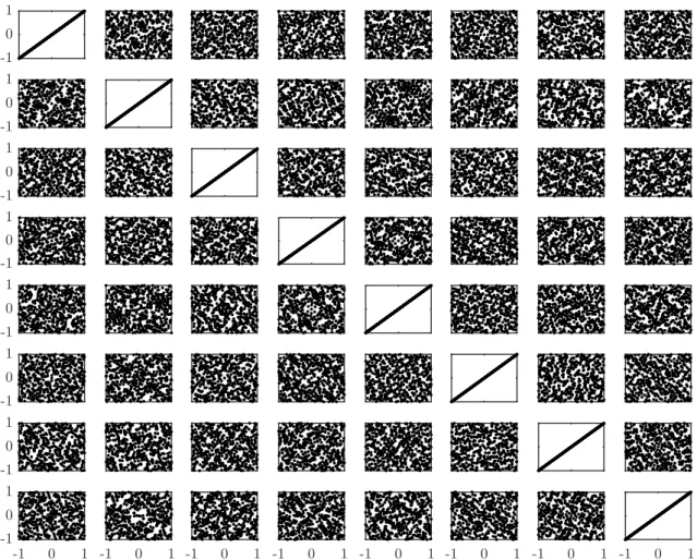
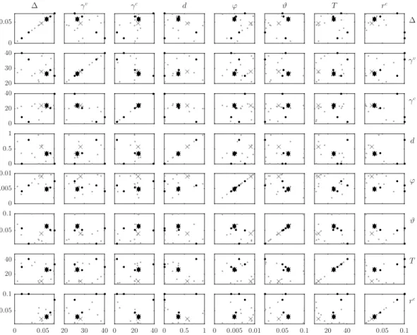
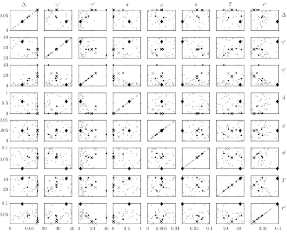
Using the extension procedure outlined in Cioppa (2002), a 513×8 design matrix is constructed from the basic 129×22 matrix provided in appendix D of that paper. A two-way scatter plot of the sample is provided in Figure 1. The first benefit of using the NOLH sampling approach for the analysis carried out here is that it provides flexibility around the central calibration of the model parameters thus enabling the comparison of the same model calibration to 31 empirical data series.
-1 0 1 -1 0 1 -1 0 1 -1 0 1 -1 0 1 -1 0 1 -1 0 1 -1 0 1 -1 0 1 -1 0 1 -1 0 1 -1 0 1 -1 0 1 -1 0 1 -1 0 1 -1 0 1
Figure 1: Scatter diagram with 513 samples from an 8-dimensional parameter space. Shown are the projections ofR8onto the 2-parameter subspaces inR2.
with respect to variations in the parameter values, essentially providing a confidence interval over the parameter space. This will be important in evaluating the ability of the MIC to discriminate amongst candidate calibrations, which is the main objective of this experiment.
3.3
Surrogate modelling: Stochastic Kriging
As previously stated, one of the aims of this paper is to evaluate the ability of the MIC to serve as the basis for the generation of a response surface in the parameter space, through the use of a surrogate model (also known as a meta-model). The motivation is that for large agent-based models the high dimensionality of the parameter space and the emergent behaviour of the model make it computationally prohibitive to specify an I/O mapping from the inputs (model parameters) to outputs (target variables). Instead, the literature suggests to use a surrogate model to approximate the responses of the full-scale ABM. In our case, the aim is to provide a surrogate model for the MIC values over the parameter space in order to identify good parameter calibrations.
Following the suggestion by Salle and Yıldızo˘glu (2014) we select stochastic kriging as our surrogate modelling methodology. The main justification for this is theoretical, as kriging is known to provide the best linear unbiased prediction (BLUP). Furthermore, Salle and Yıldızo˘glu (2014) argue that the combination of NOLH sampling and kriging is very efficient at providing good surrogate models, due to the near-orthogonality of the sample vectors and the BLUP property. This property is highly desirable in our case given the complexity of the Eurace@Unibi model and its relatively high dimensionality in both parameters and variables.
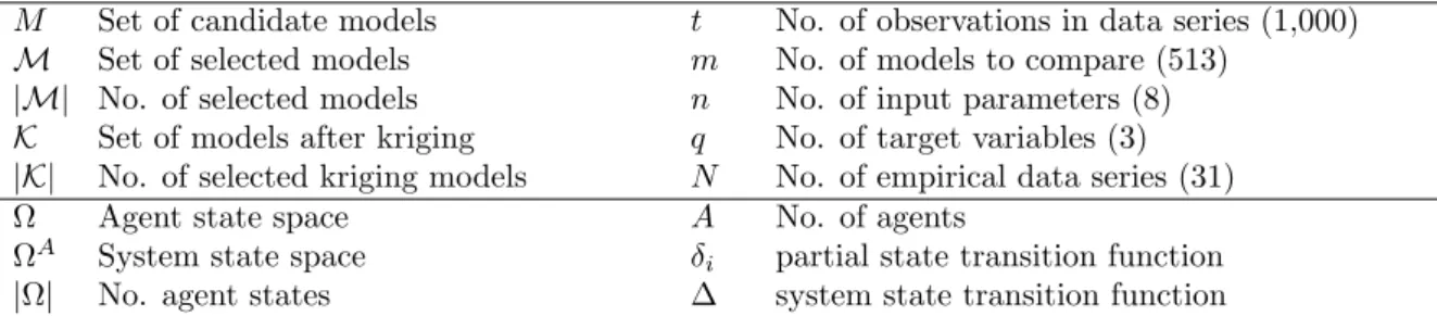
Table 1: Notation
M Set of candidate models t No. of observations in data series (1,000)
M Set of selected models m No. of models to compare (513)
|M| No. of selected models n No. of input parameters (8) K Set of models after kriging q No. of target variables (3) |K| No. of selected kriging models N No. of empirical data series (31)
Ω Agent state space A No. of agents
ΩA System state space δi partial state transition function
|Ω| No. agent states ∆ system state transition function
A second motivation for this choice is more practical, as the ooDACE toolbox for Matlab already provides kriging as a direct surrogate modelling method. Given that both the MIC and MCS approaches developed by Barde (2016a) have also been implemented in Matlab, this allows for the construction of an integrated protocol using ‘off-the-shelf’ solutions. More specifically, the procedure used for building the surrogate model for each country isstochastic kriging (SK, see Kleijnen, 2017, Sect. 5), where the MIC values obtained for each sample point are treated as noisy measurements, as opposed toordinary kriging (OK) where the observations are treated as deterministic signals. This is done to account for the fact that, as shown in Barde (2016a), the MIC measurement noisy, especially at relatively low levels of training. Using the terminology of Kleijnen (2007), the MIC measurement will already contain an element of intrinsic noise, which needs to be accounted for separately from the extrinsic noise process used by ordinary kriging.6
3.4
The validation protocol: a formal exposition
The validation protocol consists of a sequence of steps listed in Appendix 6. Below we go through these steps using a formal presentation. Table 1 provides an overview of notation. The first step is to define a simulation model as an Input/Output function, mapping model parameters into model variables. Definition 3.1. (Input/Output Function) Let a simulation model be specified bynparameters (model inputs) and by q target variables (model outputs). Imposing bounds on the parameter ranges yields a domain D ⊂Rn. Let an input signal s∈ D be an n-vector, and the corresponding output response of
the model denoted byy∈Rq. The simulation model is defined by the Input/Output function
f :D →Rq, s7→y, y=f(s). (1)
In Definition 3.2 we define the Input/Output Correspondence of a simulation model.
Definition 3.2. (Input/Output Correspondence) Let a simulation model be defined as an I/O function
f as in Def. 3.1. Further, let a set of candidate models M be given by a collection ofminput signals, denoted by S ={s1, ..., sm}, where S is an element of the sampling space S ∈ S ⊂ Rm×n. The set of
input signalsSis mapped to a set of output responsesY = (y1, ..., ym), which is an element of the output
response space Y ∈ Y ⊂ Rm×q. The setY is obtained by applying the function f element-wise to the
elements ofS, i.e. {y1=f(s1), ..., ym=f(sm)}.
TheInput/Output Correspondence (IOC) of the simulation model is a many-to-many correspondence,
6The implementation of stochastic kriging in the ooDACE toolbox in Matlab is called regression kriging. All settings of
the ooDACE toolbox are set to their default values. In particular, the bounds on the 8 hyper parameters are set to [-2,2] (in log10scale).
mapping a set of inputsS∈ S to a set of output responses Y ∈ Y:7
IOC:S → Y, S7→Y, (2) where si7→yi(si) for each i= 1, ..., m.
In the following, we will refer to the set of output responses Y as the Output Response Data of the model, given the input signalsS. In Definition 3.3 the MIC Response Surface (MICRoS) is defined, by applying the MIC-measurement function element-wise to the Output Response Data of the model. Definition 3.3. (MIC Response Surface) LetY ∈ Ybe the Output Response Data of a model, as defined in Def.3.2. Suppose we have obtained, for each of the output responses, the MIC measurement wrt. some empirical data series. The (univariate) MIC Response Surface (MICRoS) of the model is defined as the mapping:
M IC:Y →Rm, Y 7→M IC(Y), (3)
where yi,j(si)7→M IC(yi,j(si)) for each i= 1, ..., m, j= 1, ..., q,
and M IC(yi(si)) := q
X
j=1
M IC(yi,j(si)) for each i= 1, ..., m. (4)
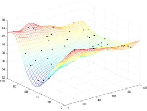
The last line (4) indicates that we consider the univariate variant of the MIC measurement of a model, by taking the sum of MIC scores across the individual target variablesj = 1, ..., q. Essentially, the MICRoS is anm-dimensional manifold embedded in an (m+ 1)-dimensional space. It consists of the realized MIC scores over the sample spaceS. Figure 2 provides an example of a 2-dimensional response surface and its interpolation surface (Couckuyt et al., 2014). Note that the black dots correspond to the response surface proper, while the smooth surface is the interpolated response surface. For the experiment in this paper, the parameters are: m= 513,n= 8,q= 3, and the number of empirical data series (OECD countries) isN = 31. Since in our case the MIC Response Surface is an 8-dimensional manifold embedded in a 9-dimensional space, we cannot easily provide a visualization for it.
Note that the MIC measurements do not constitute an estimation method as such since they only provide us with a metric of the distance between a simulated data series and an empirical data series. Note however that the MIC Response Surface can give us some information about promising not-yet sampled calibration points that lie in between the points that we have actually sampled. To provide us with predicted MIC scores for such non-sampled points in the parameter space, we adopt a statistical surrogate modelling approach that provides us with an interpolation function over the MIC scores.8
Specifically, this interpolation is carried out by applying stochastic kriging to the MIC Response Surface obtained in Def. 3.3. This final step is formally described in Def. 3.4.
Definition 3.4. (Interpolated MIC Response Surface) Let a MIC Response Surface be anm-dimensional manifold, as defined in Def.3.3. Applying stochastic kriging as the interpolation function over this man-ifold yields a continuous sub-manman-ifold ofRm. The result of this interpolation is called the interpolated MIC Response Surface, given by:
k:Rm→Rm, M IC(Y)7→k(M IC(Y)). (5)
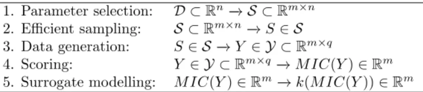
Here the function k(.) represents the application of stochastic kriging to the MIC Response Surface. The entire validation protocol can now be summarized by the sequence of steps in Table 2 (see Appendix 6 for a pseudo algorithm).
7In the above definition, the collection of model output responsesy(s) is defined in terms of the ‘target variables’ yj.
Such target variables may refer either to variables that are directly observable from the model output (for example, the unemployment rate), or may refer to derived variables constructed after the simulation data has been obtained (target
Table 2: Sequence of steps for the protocol. 1. Parameter selection: D ⊂Rn−→ S ⊂Rm×n 2. Efficient sampling: S ⊂Rm×n −→S∈ S 3. Data generation: S ∈ S −→Y ∈ Y ⊂Rm×q 4. Scoring: Y ∈ Y ⊂Rm×q−→M IC(Y)∈ Rm 5. Surrogate modelling: M IC(Y)∈Rm−→k(M IC(Y))∈ Rm
Next, given the interpolated MIC Response Surface, we try to find all local minima of this surface using a constrained optimization algorithm. This is the final step of the protocol, and is done in order to identify promising new sample points that lie outside of the initial 513 NOLH sample points.9 The reason we cannot simply take the global minimum of the interpolated surface is due to the intrinsic noisiness of the MIC measurement as a measure for the relative Kullback-Leibler distance, which could result in selecting a false local minimum as the global minimum.
The performance of the resulting kriging model as a surrogate model for the MIC Response Surface over the sample spaceScan be evaluated using the leave-one-out cross-validated prediction error (cvpe), which is obtained by successively treating each sample point as an out-of-sample test. Formally, let ˆ
ki(M IC(y)) be the kriging predictor for the interpolated MIC Response Surface at sample point si,
obtained by applying Def. 3.4 to the set of m−1 responses that excludes yi. The cvpe is obtained by
calculating the squared deviation between this leave-one-out predictor and the actual MIC measurement atsi, as follows: cvpe= 1 m m X i=1 M IC(yi)−ˆki(M IC(y)) 2 (6) A lower value of the cvpe indicates that the kriging model is better at predicting MIC scores out-of-sample across the interpolated MIC response surface.
4
Application of the protocol
4.1
A brief overview of the Eurace@Unibi artificial macroeconomy
Below we give a brief and general overview of the Eurace@Unibi macroeconomic model. For the most up-to-date model description we refer to Dawid et al. (2016). An overview of the results from various policy applications is given by Dawid et al. (2017).
Consumption goods producers’ production output decision. A typical Eurace@Unibi model economy contains 80 firms producing consumption goods. The output level of firm i is determined according to a Leontief production function with complementarity between physical capital and human variables could for instance be ratios of certain macroeconomic variables such as the debt-to-GDP ratio). Also, the target variable could refer to any statisticsm(Y) that are constructed from the simulated data series (see Windrum et al., 2007).
8It is quite likely that the interpolation of the MIC Response Surface only works well in between the set of sample points
already sampled, but not in regions outside of the sampled subspaces. This is another argument why we need to ensure a good initial coverage of the parameter space, and hence the combination of NOLH + SK seems to be a perfect match, as explained by Salle and Yıldızo˘glu (2014).
9In practice, this is carried out using Matlab’s build-infminconfunction. The minimization process converges fast and
without errors, but is sensitive to the starting point, indicating the presence of local minima in the response surface. In order to ensure robustness, the optimization procedure is run with 1,000 different random starting points within the sample space. For each local minimum found, a count is kept of the number of initial conditions in its basin of attraction, and only those local minima are kept that attract at least 10 out of 1,000 initial conditions. In other words, the basin of attraction of the local minima should have a mass of at least 1%. This ensures only those local minima with a significant basin of attraction are selected.
Figure 2: Illustration of a model’s response surface. Black dots denote the output response of the model at selected sample points. In this example, the model’s output is used directly to obtain a 2-dimensional interpolation surface. In our validation protocol, however, we need an intermediary step to compute the MIC scores, and then we interpolate over these to obtain the MIC Response Surface. Source: Lophaven et al. (2002, p.22).
capital, given by:
Qi,t= V X v=1 min " Ki,tv ,max " 0, Li,t− V X k=v+1 Ki,tk ## | {z }
effective no. machines used of vintagev
× min [Av, Bi,t] | {z } effective productivity , (7)
wherevdenotes the different vintages of physical capitalKi,tv , with newer vintages being of higher quality and therefore possessing a higher productivity per unit of capital. Li,t denotes the workforce and Av
denotes the productivity of capital of vintage v. Finally, Bi,t denotes the average productivity of the
firm’s employees, determined by the average specific skill level of the workforce. Note that the sum outside of the outer brackets goes over the vintagesv, so that we first determine the contribution of each vintage in isolation, and then sum over these to obtain the total production quantityQi,t. The individual
contributions consist of two terms: the effective number of machines of vintagevbeing used to produce, and the effective productivity of these machines, which depends on the average productivity of labour and capital due to the complementarity of these two input factors. In the first term of the overall product, i.e. in the effective number of machines used,Kv
i,t is the number of units of physical capital of vintagev
that need to be operated by employees in a 1:1 ratio, demonstrating the complementarity in real terms. In productivity terms, the complementarity shows itself in the second term of the product, min [Av, B
i,t].
Households’ consumption choice. The default model economy is populated by 1600 households and the consumption decision of households is described by a discrete choice model. McFadden (1973, 1980) has shown that the conditional choice probabilities of a population of consumers can be derived as rational choice behavior of an individual consumer, by adopting a random utility framework. Let the utility of consumerhfrom consuming goodibe given by the random utility function
uh(pi,t) = ¯uh−γcln(pi,t) +h,i,t, (8)
where ¯uh is the base utility of the product (identical across firms) and h,i,t captures the contribution
of the (horizontal) product properties of product i to the utility of consumer hin period t. The term −γcln(p
i,t) represents the fact that consumers prefer cheaper products to more expensive ones, assuming
they cannot discern any quality differences.
Assuming that in each period each consumer chooses the product with the highest utility and that
h,i,t is a random idiosyncratic term following an extreme value distribution, McFadden has shown that
the conditional choice probability of consumerhfor productiis given by
P[Consumerhselects producti] = exp (−γ
cln(p i,t))
P
jexp(−γcln (pj,t))
Here the parameterγcdenotes the price sensitivity of consumers wrt. price differences between the goods
to choose from. This parameter can also be interpreted as the intensity of price competition between the consumption goods producers in the model.
Consumption goods producers’ investment decision. For the investment decision the firm needs to decide how much to invest, but also what vintage to purchase. For the latter choice, the firm considers the ratio between the effective productivity of a particular vintage, ˆAef fi,t (v), and its price,pv
t. The vintage
choice then follows a similar specification as used for the consumer’s choice described above, with the conditional choice probability by firmi for vintagevgiven by:
P[Firmiselects vintagev] =
exp γvln ˆ Aef fi,t (v) pv t P vexp γvln ˆ Aef fi,t (v) pv t . (10)
Banks’ interest rate setting on firm loans. There are typically 20 banks in the economy that provide deposit accounts for households and firms, and maintain the payment settlement system. All money in the Eurace@Unibi artificial economy is stored in bank deposit accounts as electronic money, and all transfers are electronic as well, so there is no need for cash money in the usual sense. Banks provide credit to firms in order to finance their production or to make other payments (for instance, for debt servicing or dividend payouts). However, in the default model implementation, only the consumption goods producers can apply for loans. Household cannot get consumptive credits or mortgage loans to purchase real-estate. Also, the investment goods producer does not need any loans since it does not use any labour or capital inputs to produce, and the investment goods (machines) are produced on demand, so it also does not need any money to make advance payments.
The total volume of credit that can be created by the banks is restricted by banking regulations, possibly resulting in credit rationing for the firms. The floor level for the interest rate on commercial loans is given by the Central Bank’s base rate rc (the policy rate). This is supplemented by a mark-up
on the base rate that depends on the financial health of the firm, which is an increasing function of the firm’s financial leverage (debt-to-equity ratio). The bank’s own funding costs play only a minor role in the interest rate offered to borrowers and are added as a random idiosyncratic termbtfor each new loan contract. The bank’s offered interest rate is given by:
ri,tb =r c 1 +λB·P Dk,tb + b t , where bt∼U[0,1]. (11) Here P Db
k,t is the bank’s assessment of the firm’s Probability of Default on the loan, which is given
by:
P Dbk,t= max
3×10−4,1−exp −ν(Di,t+Lbk,t)/Ei,t
, (12)
whereDi,t andEi,t denote the current debt and equity of firm i, andLbk,tis the new loan indexed byk
that is to be added to the total debtDi,t. Default values for the parameters are: ν = 0.10 and λB = 3
(these parameters are not varied in this paper).
Labour market, firms’ base wage offer. The labour market is modelled as a fully decentralized market with direct interaction between individual firms and unemployed job seekers. A firm makes a base wage offer wbase
i,t , driven by labour market tightness. The firm increases its base wage offer by a
factorϕif it is unable to fill all open vacancies:
wi,tbase+1= (1 +ϕ)wi,tbase. (13)
Thus, the parameter ϕ reflects the firm’s willingness to pay for higher wages in case of labour market tightness.
4.2
Parameter selection and parameter calibration
In this subsection we provide more information on the design of experiments, which parameters were selected, how the parameter ranges were set, and what would be the influence of a variation of a parameter within the context of the model.
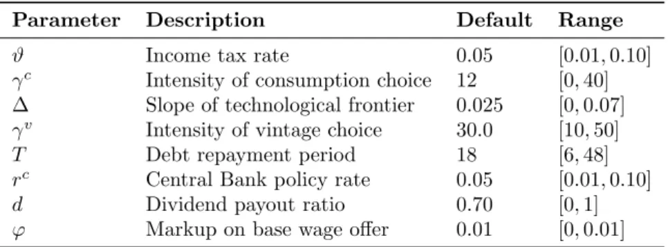
The model contains 33 parameters to model 5 markets and 1 household sector. A full list is given in the appendix in Table 13. From this list, eight parameters were selected to be used for the empirical validation experiment in this paper. These eight parameters are listed in Table 3. The parameter ranges were set based on domain knowledge and previous model explorations by the original authors of the model. Below we describe the influence of each of the eight selected parameters.
First, the income tax rateϑfor the household sector is the tax rate on all forms of household income, including wages, unemployment benefits, dividend income from share holdings and interest income from bank deposits. Higher values of ϑ signify less disposable income and lower purchasing power for the household. Hence, this will typically result in lower demand, lower output and higher unemployment rates.
Second, on the consumption goods market, the parameterγc is the logit parameter in the conditional
choice probability of the households’ consumption choice problem. In (9) this parameter reflects the sensitivity of consumers wrt. differences in prices between multiple firms selling the same consumption good in the Mall, and measures the intensity of price competition on the market. Higher values of γc
signify a more competitive market, typically resulting in a more unstable economy due to lower profit margins.
Third, on the investment goods market we select two parameters. The first is the parameter ∆ controlling the slope of the technological frontier, which is reflected by a jump in the productivity of the best-practice technology after a successful innovation. Note that the occurrence of innovations is stochastic. Higher values of ∆ signify a greater jump in technological progress, typically leading to higher productivity of the capital stock of the consumption goods producers. But note, however, that only those firms that actually invest in the new vintage will benefit from this increased productivity. Also, since the productivity of physical capital is complementary to the productivity of the labour force in the Leontief production function (7), the firm needs to hire workers with higher specific skill levels in addition, to take advantage of the increased physical capital productivity. The parameter value of ∆ is also used to increase the price of the new vintage when it enters the market. Therefore a higher value of ∆ will also mean that investments in the current best-practice technology becomes more expensive, which might lead some consumption goods producers to rather invest in older vintages first. Hence, the diffusion of new technologies could slow down for higher values of ∆.
Fourth, the second parameter we select on the investment goods market is γv, which is the logit parameter in the conditional choice probability of the consumption goods firms, as given in (10). It controls the intensity of choice to select vintagevover any of the other vintages available. Higher values ofγv imply that a firm is more sensitive to differences wrt. the ratios between the effective productivity and the price.
Fifth, on the credit market we select two parameters as well. The first is the parameterT that reflects the length of the debt repayment period. Increasing the parameterT will give firms more time to repay their debts, but it will also lead to more leverage. In tranquil times this will lead to higher levels of production and more investments, but in times of crisis it results in more financial instabilities.
Sixth, the second parameter on the credit market that we select is the Central Bank base rate rc. In
(11) higher levels ofrclead to higher interest rates on deposits and to higher interest rates on commercial
loans. The overall effect is therefore ambiguous, as it may lead to higher income flows for households and firms alike on their deposit accounts through the interest channel, but it may also lead to higher interest payments for firms that need to service their debts.
Seventh, on the financial market we select the parameterdthat sets the dividend payout ratio for all (active and profitable) firms and banks. A higher dividend payout ratiodhas a positive effect on demand since the dividends are an income flow for the household sector, and thus functions as a purchasing power enhancing effect. But at the same time dividend payout are also an expenditure for the corporate sector, so it may crowd out investments.
Finally, the eight’ parameter is ϕ, related to the labour market, which controls the factor by which firms adjust their base wage offer. In (13) a higher value ofϕsignifies that firms will increase their base
Table 3: Selected list of parameters from the Eurace@Unibi model used in this paper.
Parameter Description Default Range
ϑ Income tax rate 0.05 [0.01,0.10]
γc Intensity of consumption choice 12 [0,40]
∆ Slope of technological frontier 0.025 [0,0.07]
γv Intensity of vintage choice 30.0 [10,50]
T Debt repayment period 18 [6,48]
rc Central Bank policy rate 0.05 [0.01,0.10]
d Dividend payout ratio 0.70 [0,1]
ϕ Markup on base wage offer 0.01 [0,0.01]
wage by a greater percentage in case they are unable to fill their open vacancies. Under conditions of labour market tightness this might lead to wage push inflation.
4.3
Simulation: Generation of the training data
Our use case has multiple parameter sets (typicallym= 513 sets) and multiple Monte Carlo replication runs per set (typically 1,000 runs per set). This yields an embarrassingly parallel computing problem, since all the individual simulation runs are independent from each other. Therefore they can be arbitrarily distributed across many compute nodes, and launched as a distributed computational problem on a computing cluster.10
The simulated data is divided into two sets, an in-sample data set consisting of 99% (990 series per NOLH sample) and an out-of-sample data set for the remaining 1% (10 series per NOLH sample), for each of the 513 NOLH samples. The 99% set forms the training data that is used by the CTW algorithm to build the set of 513 context trees corresponding to each calibration. The trees encode the reconstructed Markov transition matrices that can be used to extract the conditional probabilities required to score the calibrations on the empirical data. The out-of-sample 1% set is used for an internal validation exercise, in order to investigate whether the training data is sufficient to give the MIC discriminatory power over the 513 NOLH samples. Such an internal validation exercise could be seen as an out-of-sample prediction test. The exercise uses each trained context tree to score the 513 ×10 runs belonging to the out-of-sample data set in order to establish whether the trees are able to identify the specific calibration they were trained on. If this is the case, then we can conclude that the MIC is able to discriminate between the calibrations, thus validating the training stage.
4.4
Empirical data
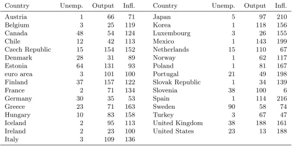
The macroeconomic data are used for the empirical calibration exercise covers 30 OECD countries and the euro area. We use three target variables (the names in parenthesis refer to variable names in the Eurace@Unibi model): the harmonized monthly unemployment rate (unemployment rate), the monthly year-on-year growth rate of industrial production, considering only the manufacturing sector (output growth rate), and the monthly year-on-year growth rate of the CPI (inflation rate). The relatively large number of countries examined and the choice of a monthly data frequency are both motivated by the desire to have as large an empirical data set as possible, in order to facilitate the statistical analysis of the MIC scores using the MCS procedure.
A basic description of the data, including the countries used, number of observations and bounds for each series, is provided in Table 9 in appendix C. All data series are taken from the Stats OECD website,
10We have used a simple round-robin algorithm (like card shuffling) to allocate the runs to a fixed number of job lists.
We used 4750 job lists consisting of 9 consecutive blocks of 12 runs each, yielding 108 runs in total per job list. Each job list takes almost exactly 2 hours of wall-time to complete on a compute node with 2 Westmere hexa-core processors (Xeon
and the start date corresponds to the point in time at which all three data series became available.11 The
harmonised unemployment rate data is directly available as a monthly rate, whereas the growth rates of manufacturing production and the CPI were downloaded as monthly index values and then transformed into monthly year-on-year growth rates by the authors. Similarly, the simulation data for aggregate firm output and the price index are produced as monthly values first, and then need to be transformed into monthly year-on-year growth rates before we start the validation protocol.
Because the MIC methodology treats both empirical and simulated data sets as if they are the output from a Markov process, all data series need to be discretized before the methodology can be applied. This requires choosing a set of bounds to define the support of each variable, as well as a choice of resolution
r, in order to determine the number of discrete states of each variable (2r). Discretizing the support of the target variables implies that information is inevitably discarded. However, as explained more fully in Barde (2016a), the MIC is not affected by the discretization procedure if the discretization error is pure white noise, i.e. distributed as an i.i.d. uniform random variable. As a result, one can check that a given choice of bounds and resolution are appropriate for the procedure by testing the error term for this.
The main difficulty encountered in the procedure is to set ranges on the target variables to account for the variability reported in Table 9. The resolution is set tor = 7 bits for all three variables while the unemployment rates are restricted to [1%,25%], manufacturing output growth rates are restricted to [−30%,30%] and the inflation rates are restricted to [−2%,20%], with any out-of-bounds observations taking the value of the corresponding bound. Tables 10, 11 and 12, also in appendix C, display the results of the discretization tests for these values of the upper and lower bounds and resolution. The Komogorov-Smirnov test is used to check that the discretization error is uniformly distributed, while two Ljung-Box tests are used to test for independence, one by testing for autocorrelation in the discretization error itself, the other by testing for cross-correlation of the error with the discretized variable.
These tables show first of all that the combination of bounds and resolutions are sufficient in nearly all cases to ensure that the discretization error is uniformly distributed. The few cases where this is not the case, such as the unemployment series for Greece, or the inflation series for Ireland and Mexico, seem to occur due to the relatively large number of out-of-bound observations. Autocorrelation of the discretization error does not seem to be a problem for unemployment, and to a lesser extent for manufacturing output growth, however quite a few countries fail the test for CPI inflation. The test that performs poorest for all three variables is the correlation with the discretized variable, suggesting that the discretization error still contains information with respect to the state variable. However, if the error is uniform and not autocorrelated, this is less of an issue as long as the correlation is low. Of the 21 failed cross-correlation tests over the 3 variables and 31 series, only six have an absolute Pearson correlation coefficient above 0.1, and the largest case observed is -0.134 for unemployment in Chile.
5
Results
5.1
Internal validation of the MIC
As explained in Section 4.3, after the first stage in which we compute MIC scores using 99% of the training data (for each NOLH sample separately), an internal validation test is carried out using the remaining 1% of the training data, in order to verify that the training data is sufficient to give the MIC discriminatory power over the 513 NOLH samples. This internal validation step is not required in order to obtain the MIC scores on the empirical data, but it is helpful as an intermediate confirmation of the robustness of the training data set.
The internal validation is carried out by treating the simulated runs in the 1% training data set as if they were empirical data. We use these to obtain the MIC score for each of the 513 trees that result from the CTW algorithm on the 99% training data set, for all 3 macroeconomic variables. The 1% training data set consists of 513×10×3 series, corresponding to the set of 513 calibrations, the 10 runs in the sample and the 3 variables in the analysis. For each of these series, the internal validation test provides a MIC score for each of the 513 trees generated by using the 99% training data set.
As this is a large set of test scores, the results are summarised using two main statistics. The first is the rank attributed to the ‘true’ calibration, i.e. the rank given where the training and testing calibrations