Federated Matrix Factorization: Algorithm
Design and Application to Data Clustering
Shuai Wang and Tsung-Hui Chang November 2, 2020
Abstract
Recent demands on data privacy have called for federated learning (FL) as a new distributed learning paradigm in massive and heterogeneous networks. Although many FL algorithms have been proposed, few of them have considered the matrix factorization (MF) model, which is known to have a vast number of signal processing and machine learning applications. Different from the existing FL algorithms that are designed for smooth problems with single block of variables, in federated MF (FedMF), one has to deal with challenging non-convex and non-smooth problems (due to constraints or regularization) with two blocks of variables. In this paper, we address the challenge by proposing two new FedMF algo-rithms, namely, FedMAvg and FedMGS, based on the model averaging and gradient sharing principles, respectively. Both FedMAvg and FedMGS adopt multiple steps of local updates per communication round to speed up convergence, and allow only a randomly sampled subset of clients to communicate with the server for reducing the communication cost. Convergence analyses for the two algorithms are respectively presented, which delineate the impacts of data distribution, local update number, and partial client communication on the algorithm performance. By focusing on a data clustering task, extensive experiment results are presented to examine the practical performance of both algorithms, as well as demonstrating their efficacy over the existing distributed clustering algorithms.
Keywords−Federated learning, matrix factorization, model averaging, gradient sharing, clustering.
I. INTRODUCTION
Matrix factorization (MF) is one of the most fundamental models which has vast applications in signal processing and machine learning, including data clustering, dimension reduction, item recommendation, hyperspectral unmixing, and biological analysis, to name a few [1], [2], [3]. Mathematically, a general MF problem is formulated as follows
min
W,H Φ(X,WH) +RW(W) +RH(H) (1a)
s.t. W∈ W,H∈ H, (1b)
Shuai Wang and Tsung-Hui Chang are with the Shenzhen Research Institute of Big Data and School of Science and Engineering, The Chinese University of Hong Kong, Shenzhen 518172, China (e-mail: [email protected], [email protected]).
whereX∈RM×N is the observation data,W∈RM×K andH= [h
1, . . . ,hN]∈RK×N are two matrix
factors, andW andHare some constraints, andRW(·)andRH(·)are regularization functions forWand
H, respectively. The cost functionΦ(X,WH)measures the quality of the approximationX≈WH; for example,Φ(X,WH) = N1kX−WHk2
F is a popular cost function used in many applications. In view of
the increasing volume of real-life data, distributed MF methods that can process large-scale datasets have gained significant interests in the last decade [4]. However, recent emphasis on user privacy has called for new distributed schemes that can realize these MF based applications without revealing the users’ private data. Specific examples include processing distributed patient medical records stored in multiple hospitals [5] and daily personal data of mobile users [6].
As an emerging distributed learning paradigm, federated learning (FL) has been introduced by Google to enable collaborative model learning over distributed data owned by massive clients (e.g., mobile devices or institutions). The FL runs under the orchestration of a central server without the need of knowing the clients’ raw private data. Compared with traditional distributed learning schemes [7], FL faces new challenges. This includes dealing with massively distributed clients in heterogeneous networks which have unbalanced and non-i.i.d. data distribution, and limited communication resource for message exchanges between the server and clients [6].
To train a model under the challenging FL setting, serveral FL algorithms have been proposed [8], [9], [10], [11], [12], mostly based on the classical stochastic gradient descent (SGD) method. In particular, [8] proposed a model averaging algorithm, called FedAvg, where the server coordinates the training by iteratively averaging the local models learned by the clients via SGD. A salient feature of FedAvg over the classical gradient sharing approach is local SGD, where the clients are allowed to perform multiple epochs of SGD locally before sending the local model to the server for averaging. Local SGD has been proven an effective strategy to reduce the required number of communication rounds for producing a good model [8], [11], [12]. The second feature of FedAvg is partial client participation (PCP), where only a small number of clients are sampled and communicate with the server in each communication round. Partial participation can greatly alleviate the network congestion problem especially when the number of clients is large and communication bandwidth is limited. It also models that a client might become offline randomly due to poor link quality. We notice that, while many successful efforts have been made for supervised FL tasks, few works have been done for the MF model (1) and its applications.
A. Related Works
For example, the recent works [13] and [14] studied the federated MF (FedMF) problem for recom-mendation systems. They considered the gradient sharing strategy, where, in each communication round,
the server aggregates the gradient information of the cost function from the clients and applies one step of gradient descent for model training. However, as mentioned in [8], the gradient sharing based methods would require a large number of communication rounds to produce a good model. It is also worth noting that the existing model averaging based FL algorithms [8], [9], [10], [11], [12] are not directly applicable to problem (1) because these existing studies have assumed smooth and unconstrained problems while (1) is constrained, and the existing algorithms are designed to deal with problems with single-block variable while (1) involves two blocks of variables.
On the other hand, although many distributed MF methods have been proposed, they did not consider the FL scenario and address the associated issues. Specifically, a large body of the existing distributed MF methods are parallel implementations of the centralized sequential SGD or alternating least square (ALS) algorithms, either on MapReduce [15], [16], [17] or Parameter server [18]. Analogously, parallel implementations of the multiplicative rule [19] and block coordinate descent [20], [4] on MapReduce are developed for non-negative MF (NMF) models. Again, these works usually assume that there is a shared memory that all nodes can access, and careful model/data partition is required for efficient parallelization. Another category of works considered decentralized MF methods such as [21], [22], [23], [24] with the absence of the central server. Consensus methods are often used to achieve distributed optimization. However, the critical issues of FL such as unbalanced/non-i.i.d. data are not considered therein.
In summary, firstly, the existing FedMF and distributed MF algorithms have not been fully customized to overcome the challenges of FL in massive and heterogeneous networks. Secondly, the current studies have focused on specific applications (such as item recommendation), there still lacks a systematic algorithm design for the general MF model (1) so that the designed algorithms can subsequently be employed in various MF applications. Thirdly, the existing FedMF works do not present theoretical convergence analysis and thus are not able to analytically explain how various factors, such as non-i.i.d. data distribution and partial communication, can affect the algorithm performance.
B. Contributions
In this paper, we aim to investigate communication-efficient FedMF algorithms. In particular, we propose two novel FedMF algorithms, based on the principles of model average (MA) and gradient sharing (GS), respectively. We assume thatWis a shared variable of all clients whereasHcan be (column-wise) partitioned into multiple local variables exclusively owned by respective clients; see Section II for the detailed FedMF model.
1) We firstly propose a new FedMF algorithm, called FedMAvg, that judiciously combines the al-ternating minimization method and the MA technique, where the former is a popular method for
handling the MF model in (1) [25]. Specifically, in each communication round of FedMAvg, the clients perform one round of local alternating minimization through multiple steps of local projected gradient descent (local PGD) with respect toH andW, followed by averaging the locally learned modelWat the server. Besides, partial client communication (PCC) is adopted to reduce the overall communication cost, where only a sampled subset of clients upload their models to the server in each round. We present a convergence analysis which explicitly characterizes how the number of local updates, PCC and non-i.i.d. data distribution can affect the algorithm convergence. The analysis suggests that adiminishing number of local updates should be used for FedMAvg so that it can be less sensitive to non-i.i.d. data. Unlike the existing analyses [8], [9], [10], [11], [12] which are for smooth unconstrained problems, our analysis overcomes the challenge due to the constraints and two-block variables in problem (1).
2) Secondly, we propose a new GS based FedMF algorithm, called FedMGS, which improves upon the algorithms in [14], [13] in terms of convergence speed and communication efficiency. In FedMGS, the clients are responsible for computing∇WΦand uploading it to the server which is in charge of
updatingW. We focus on MF problems with the squared Frobenius norm cost, i.e., Φ(X,WH) =
1
NkX−WHk2F. By exploring the fact that∇WΦhas a linear separable structure, one can allow both
the clients and the server to perform multiple steps of PGD in each communication round, which thus can improve the convergence speed in a way similar to MA based methods. Analogously, in FedMGS, we allow only a sampled subset of clients to be active and communicate with the server, which reduces the communication cost. Convergence analysis reveals that FedMGS is inherently resilient to non-i.i.d. data distribution.
To examine the performance of the proposed FedMF algorithms, we apply them to the federated data clusteringtask and test them on both synthetic dataset and real datasets including the TDT2 document data [26], the TCGA cancer gene data [27], and the MNIST hand-writing digits data [28]. Extensive experiment results are presented, which not only provide useful insights on how various algorithm parameters and data distribution affect the algorithm performance, but also show the superiority of the proposed algorithms over the existing distributed clustering methods.
Synopsis:Section II presents the FedMF problem model and its application to data clustering. Section III and Section IV respectively present the proposed FedMAvg and FedMGS algorithms and their convergence analyses. Experiment results are presented in Section V, and lastly the conclusion is drawn in Section VI.
Notation: Rm×n denotes the set of m by n real-valued matrices. The (i, j)th entry of matrix A is
vector, andIm is them by m identity matrix, and k · kF is the matrix Frobenius norm.hA,Bi denotes
the inner product between matricesA and B. λmax(A) stands for the maximum eigenvalue of A.
II. FEDERATEDMFANDAPPLICATION TOCLUSTERING A. FedMF Model
By considering the FL setting, we assume that the data matrix can be partitioned asX= [X1,X2, . . . ,XP]
and respectively owned by P distributed clients. Specifically, each client p owns non-overlapping data
Xp ∈RM×Np, whereNp is the number of samples of client p andPPp=1Np =N. Besides, we assume
that there is a server who coordinates the P clients to accomplish the MF task with all the distributed
data X1,X2, . . . ,XP being considered. Note that, under the FL scenario, the number of clients P could
be large, the data size Np, p = 1, . . . , P, could be unbalanced, and the data samples X1,X2, . . . ,XP
could be non-i.i.d. [29], [6].
Let H = [H1, . . . ,HP] be partitioned in the same fashion as X, and let ωp = Np/N, p ∈ P ,
{1, . . . , P}. Moreover, assume thatΦ(X,WH) =PPp=1Φp(Xp,WHp), RH(H) =PPp=1RH(Hp)and
H=H1× H2· · · × HP which are separable with respect to H1, . . . ,HP. Then, one can write the MF
problem (1) as min W,Hp, p=1,...,P F(W,H), P X p=1 ωpFp(W,Hp) (2a) s.t.W∈ W,Hp ∈ Hp,∀p∈ P, (2b) where Fp(W,Hp) = Φp(Xp,WHp) ωp + RH(Hp) ωp +RW(W) (3)
is the local cost function of each client p. As seen, W is a shared variable whereas Hp, p ∈ P, are
client local variables.
The FedMF algorithm should enable the server to coordinate the distributed clients to jointly solve the MF problem (2) without the need of the clients revealing their private raw data. We should emphasize here that problem (2) is much more challenging to solve than the FL problems considered in the literature [8], [9], [10], [11], [12] because problem (2) is non-convex and non-smooth (due to the constraints) and problem (2) involves two blocks of variablesWandH. Thus, the existing FL algorithms that are designed for smooth problems with single-block variable cannot be applied to problem (2). In addition, the GS based methods in [13] and [14] are not communication-efficient solutions to problem (2), as mentioned in Section?? and will be verified in Section V.
B. Federated Clustering via FedMF
As mentioned, the MF model (1) has many applications in signal processing and machine learning. In this paper, we are particularly interested in applying the MF model (1) for data clustering, in view of that clustering is one of the most fundamental data mining tasks.
Take clustering as the example. When Φ(X,WH) = N1kX−WHk2
F, RW(W) =RH(H) =0 and
H={H | 1>hj = 1, [H]ij ∈ {0,1}, ∀i= 1, . . . , K, j = 1, . . . , N}, the MF model (1) corresponds to
the classical K-means formulation [1]. Specifically, in (1), columns of W represent centroids of theK
clusters, while H ∈ H is the cluster assignment matrix where [H]ij = 1 indicates that data sample xj
is uniquely assigned to cluster i. Thus, the K-means algorithm is equivalent to solving the above MF problem (1) via alternating minimization [30]. Interestingly, recent studies have shown that structured MF models such as the orthogonal non-negative MF (NMF) [1], [31] can outperform the K-means in many application scenarios.
However, there lacks algorithms that can perform clustering in FL network. In the literature, there are two main categories for distributed clustering. In the first category, the methods are simply parallel implementations of the centralized clustering algorithms, such as K-means [32], [33], [34] and density based DBSCAN [35], but they usually assume a shared memory, which is opposite to the setting of FL. Distributed clustering methods in the second category target at approximating the centralized clustering methods via constructing so-called coreset, which is a small-sized set of weighted samples whose cost approximates the cost of the original dataset. Thus, clustering over the coreset is approximately the same as clustering over the original dataset, which resolves the large-scale clustering issue. For example, in [36] distributed clients generate local coresets based on local data, and their union constitutes a global coreset, while in [37], a global coreset is directly constructed from locally clustering results. Impressively, these methods are communication efficient since the clients require to communicate with the server for one or two rounds only. Approximation ratios with respect to the referenced algorithms (such as K-means/K-median/K-centers) are also guaranteed [37], [36], [38], [39]. However, these coreset methods are in general no better than their referenced algorithms.
In the next two sections, we present the proposed FedMF algorithms, and then examine their practical performance on the data clustering task in Section V.
III. FEDERATEDMFBYMODELAVERAGING
In this section, we develop a MA based FedMF algorithm, termed FedMAvg, and establish its theoretical property.
A. FedMAvg Algorithm
Straightforward application of the MA technique to the distributed MF problem (2) would lead to an iterative algorithm as follows. For round s= 1,2, . . ., each client p obtains an approximate solution to
the corresponding local subproblem of (2), i.e.,
(Wps,Hsp) = arg min W,Hp
Fp(W,Hp) (4a)
s.t. W∈ W,Hp ∈ Hp. (4b)
Since W in (2) is the shared variable, the server collects and takes certain average of Ws1, . . . ,WPs, denoted by Ws, and broadcasts the average Ws to the clients for the next round of updates.
There are many possible ways to handling problem (4). One approach is simply employing one step of the alternating minimization; that is, givenWs−1 in the previous round, each clientp performs
Hsp = arg min Hp∈Hp Fp(Ws−1,Hp), (5a) Wsp = arg min W∈W Fp(W,H s p). (5b)
In practice, it is sufficient to employ the simple PGD method for (5a) and (5b), respectively. In particular, by following the same spirit as the multiple-step local SGD in FedAvg [8], we propose to approximate (5a) byQ1 ≥1 consecutive steps of PGD with respect toHp, i.e., for t= 1, . . . , Q1,
Hs,tp =PHp Hs,tp −1− 1 cs p∇ HpFp(W s−1,Hs,t−1 p ) , (6)
where Hs,0p =Hsp−1; ctp>0is the step size, and PH denotes the projection operation onto the sets Hp.
Denote Hs
p =Hs,Qp 1 for all p∈ P.
Analogously, we approximate (5b) by Q2≥1consecutive steps of GD (no projection) with respect to
W, i.e., fort=Q1+ 1. . . , Q,
Wps,t=Ws,tp −1− 1
ds∇WFp(W s,t−1
p ,Hs,Qp 1), (7)
where Q= Q1+Q2 and ds > 0 is a step size. After a total number of Q local model updates, each
clientp sends its local model of Wsp =Ws,Qp to the server. The server takes the weighted average and
applies projection operationPW to it
Ws=PW XP p=1 ωpWps−1,Q . (8)
Diminishing Q2: As W is the shared variable, the local GD length Q2 should not be too large since
especially in the presence of heterogeneous non-i.i.d. data. This insight was also found in the classical FedAvg algorithm [8], [11], [12]. To overcome the issue, we propose to consider a diminishing Q2; for
example, we consider Qs
2 = b
ˆ Q
sc+ 1, where Qˆ is a preset number. The intuition is that in the early
iterations the clients should “explore” more by performing more GD updates based on its local data, whereas when the algorithm is close to convergence, they should make small movements only to avoid model deviation. As will be demonstrated later by theoretical analysis and empirical experiments, the strategy of diminishingQ2 can benefit the algorithm convergence significantly.
Partial client communication (PCC): After a total number of Qs = Q
1+Qs2 local updates, each
client p sends Wps,Qs to the server for model averaging. Like FedAvg [8], we let the server samples a
small, fixed-size subset of clients (denoted by As with size |As| = m P) and ask them to upload
their local models Ws
p, p∈ As. The server then simply takes the average of the uploaded messages by
Ws=PW 1 m X p∈As−1 Wsp−1,Q , (9)
followed by projection onto W. Note that under PCC, the clients that are not selected are still active in updating their local variables by (6)-(7), which is different from the PCP[8], [12] where non-selected clients are completely inactive. It will be shown that the PCC scheme actually can provide significant performance improvement, particularly in heterogeneous networks with non-i.i.d data.
The details of the proposed FedMAvg algorithm are summarized in Algorithm 1.
Remark 1 Rather than using the alternating minimization strategy (6)-(7), one may instead approximate problem (4) by applying Q/2 consecutive proximal alternating linearization minimization (PALM) steps
[40] locally at each client p. That is, given Wps,0 , Ws, and Hs,0p , Hsp−1,Q/2 in the round s, each
clientp performs for t= 1, . . . , Q/2
Hs,tp =PHHs,tp −1− 1 cs p∇ HpFp(W s,t−1 p ,Hs,tp −1) , (15) Ws,tp =PWWps,t−1− 1 ds∇WFp(W s,t−1 p ,Hs,tp ) . (16)
The above (15)-(16) are different from (6)-(7) in the order of updates. Intriguingly, our numerical experience suggests that (15)-(16) may not be a good strategy. To gain the insight, one can see that when
Q→ ∞ the updates in (6)-(7) merely correspond to applying a single step of alternating minimization
to the local problem (4), whereas applying Q/2 PALM steps (15)-(16) with Q → ∞ would reach a
Algorithm 1 Proposed FedMAvg algorithm Input:initial values ofW0
1=· · ·=W0P at the server side, initial values of{Hp}0 Pp=1at the clients,A0={1, . . . , P}and
ˆ
Q.
forrounds= 1toS do
Server side:Compute
Ws=PW 1 m X p∈As−1 Wsp−1 , (10)
and select a set of clientsAs(with size |As
|=m) by sampling with replacement according to probabilities{ω1, . . . , ωP},
and broadcastWsto all clients.
Client side:
forclientp= 1toP in paralleldo SetHs,0p =Hps−1 andWs,0p =Ws. forepocht= 1toQ1 do Hs,t p =PHp Hs,t−1 p − ∇HpFp(W s,t−1 p ,Hs,tp −1) cs p , (11) Ws,tp =Wps,t−1. (12) end for forepocht=Q1+ 1toQs=Q1+Qs2 do Wps,t=Ws,tp −1− ∇WFp(Wps,t−1,Hs,tp −1) ds , (13) Hs,tp =Hs,tp −1. (14) end for DenoteWs p=Ws,Q s p andHsp=Hs,Q s p . ifclientp∈ Asthen UploadWs p to the server. end if end for end for
(15)-(16) would be too greedy and may not benefit the global algorithm convergence, especially in the presence of non-i.i.d. data.
B. Convergence Analysis of FedMAvg
Assumption 1 All local cost functions Fp are lower bounded, i.e., Fp(W,Hp) ≥F > −∞, ∀ W ∈
W,Hp ∈ Hp, where the constraint sets W and Hp, p∈ P, are compact and convex.
Assumption 2 Fp are continuously differentiable in both W and Hp. Moreover, ∇HpFp(W
s,·) is
Lipschitz continuous onHp with constant LsHp, and∇WFp(·,H s,Q
p ) is Lipschitz continuous on W with
constantLs Wp.
Note that by Assumption 2,∇WF(·,H)is Lipschitz continuous with constantLsW =qPPp=1ωp(LsWp)2.
SinceW and Hp are compact by Assumption 1, there exist upper and lower bounds for LsWp andLsHp,
e.g., for all p∈ P,
LW ≥LsWp≥LW >0, LH ≥L s
Hp ≥LH >0. (17)
In addition, under compact W and Hp, we can have the following bounds
k∇WFp(W,Hp)− ∇WF(W,H)k2F ≤ζ2, (18)
k∇WF(W,H)k2F ≤φ2, (19)
for allW ∈ W and H∈ H, where ζ and φ are some constants. Equation (19) means that the gradient
ofF is bounded. Equation (18) implies that the deviation between the local gradient ∇WFp and global
gradient ∇WF are also bounded. It is worth noting that the term in (18) is usually used in the FL
literature [41] to quantify the effect of non-i.i.d. data. Different from [41] where (18) and (19) are made as assumptions, in our work we have (18) and (19) to hold naturally since problem (2) is a constrained problem.
To build the convergence condition, we define the following sequence f Ws,t =PW 1 m X p∈As Wps,t , Wfs,0=Ws, (20) t= 1, . . . , Qs, as the instantaneous weighted average of local models. Besides, we define the following
terms as the optimality gap between a stationary solution of problem (2)
GH(Wfs,t,Hs,t), P X p=1 ωp(csp)2 Hs,tp − PHp H s,t p − 1 cs p∇ HpFp(Wf s,t,Hs,t p ) 2 F, ∀t∈ Q1, (21) GW(Wfs,t,Hs,t),(ds)2kWfs,t− PW Wfs,t− 1 ds∇WF(Wf s,t,Hs,t)k2 F, ∀t∈ Qs2, (22)
whereQ1 ,{1, . . . , Q1}andQs2,{Q1+1, . . . , Qs}. Note that ifGH(Wfs,t,Hs,t) =GW(Wfs,t,Hs,t) =
0, then (Wfs,t,Hs,t) is a stationary solution of problem (2). The main theoretical results for FedMAvg
Theorem 1 LetQs 2=b ˆ Q sc+ 1andT = PS
s=1Qs be the total number of gradient evaluations per client.
Moreover, letcs
p = γ21LH,ds=γ2LsW, where γ1 >1andγ2 ≥Q12
q
2(7 + 4L2W/L2W), and letAs (with
|As|=m ≤P) be obtained by sampling with probability {ω
1, . . . , ωP} with replacement. Then, under
Assumptions 1 and 2, the sequence{(Wfs,t,Hs,t)} of FedMAvg satisfies
1 T XS s=1 Q1 X t=1 E[GH(Wfs,t−1,Hs,tp −1)] + S X s=1 Qs X t=Q1+1 E[GW(Wfs,t−1,Hs,t−1)] ≤D T F(Wf1,0,H1,0)−F + 8Dζ2 mγ2LW +96ζ 2 m +2D(1 + 8/m)( 11 3ζ2+φ2) PS s=1C1s T γ3 2LW +( 11 3ζ2+φ2) PS s=1C2s T γ22 + 3(ζ2+φ2)PSs=1C1s 2T , (23) whereD, γ12LH 2(γ1−1) + 6(γ2 2+1)L 2 W (γ2−1)LW , and C1s ,Qs2(Qs2−1)(2Qs2−1), (24a) C2s ,6(3Qs2(Qs2−1)/2 + 4 + 32/m)C1s. (24b)
Proof: See Appendix A.
The bound in (23) shows that the local GD length Q1, Qs2, non-i.i.d. data ζ and PCC m all have
strong impacts on the convergence of FedMAvg. One can notice that if constant Qs2 =Q2 = 1 is used,
then PS
s=1C1s =
PS
s=1C2s = 0, which makes the last three terms in the right hand side (RHS) of (23)
vanish to zero. On the other hand, if T = SQ1 +PSs=1Qs2 is fixed, then increasing Q1 or Qs2 can
potentially reduce the required number of communication rounds S. Thus, there need proper choices of Q1 or Qs2 for a good trade off between convergence performance and communication efficiency. One
can see that if constant Qs2 =Q2 >1 is used, then both PSs=1C1s and
PS
s=1C2s linearly increase with
S and are unbounded. On the contrary, if Qs2 =bQsˆc+ 1, then one can show (see [42, Section 3]) that
both PS
s=1C1s =O( ˆQ3) <∞,
PS
s=1C2s =O( ˆQ5) <∞, and thereby the last three terms in the RHS
of (23) can decrease sublinearly when T is large. Therefore, the diminishing Q2 strategy can trade off
between convergence performance and communication efficiency in a better way than constant Q2.
It can also been seen from the 2nd term in the RHS of (23) that PCC would slow down the algorithm convergence, especially under non-i.i.d. data. Interestingly, when m increases, such negative effect can
be reduced. In fact, when |As|= |m|=P (full participation), the term 8Dζ2 mγ2LW +
96ζ2 m
vanishes, and FedMAvg can converge to a stationary solution problem (2) in a sublinear rate.
Corollary 1 Consider full participation in FedMAvg, i.e.,|As|=P, ∀s, and the use of weighted average
like (8). Let Wfs,t =PW PPp=1ωpW s,t
p for all s and t. Then, under the same setting as Theorem 1,
the sequence {(Wfs,t,Hs,t)} of FedMAvg satisfies
1 T XS s=1 Q1 X t=1 GH(Wfs,t−1,Hs,t−1) + S X s=1 Qs X t=Q1+1 GW(Wfs,t−1,Hs,t−1) ≤DT F(Wfs,0,Hs,0)−F + 1 T 3 2(ζ 2+φ2) S X s=1 C1s+( 11ζ2 3 +φ2) γ2 2 DPSs=1Cs 1 γ2LW + S X s=1 C3s . (25)
whereC3s,6(3Qs2(Qs2−1)/2 + 2)C1s, Dand C1s are defined in Theorem 1.
Proof: See [42, Section 2].
IV. FEDERATEDMFBYGRADIENTSHARING
In this section, we focus on MF models with the squared Frobenius norm loss function Φ(X,WH) =
1
NkX −WHk2F. By carefully exploiting the linear structure of ∇WΦ, we present another FedMF
algorithm, termed FedMGS, and its convergence analysis. A. FedMGS Algorithm
According to the GS principle [8], for problem (2) each client p should compute the gradient∇WFp
and upload it to the server. After collecting ∇WFp, p ∈ P, the server performs one step of PGD with
respect to W, and broadcasts the new W to the clients. More specifically, given Ws−1 at the clients, the client p computes ∇WFp(Ws−1,Hsp) where
Hsp= arg min Hp∈Hp
Fp(Ws−1,Hp). (26)
The PGD performed by the server is Ws=PW Ws−1− 1 ds P X p=1 ωp∇WFp(Ws−1,Hsp) . (27)
Analogous to (6), we can approximate (26) by Q1 ≥ 1 consecutive PGD steps with respect to Hp;
specifically, givenHs,0p =Hps−1, each client p performs for t∈ Q1,
Hs,tp =PHp H s,t−1 p − 1 cs p∇Hp Fp(Ws−1,Hs,tp −1) , (28) and obtain Hs p =Hs,Q 1
p . For example, the FedMF algorithm in [14], [13] adopts Q1 = 1. However, as
pointed out in [8], the GS scheme will need a lot of communication rounds to produce a good model. To overcome this, we not only require Q1 >1, but also require the server to perform multiple steps of
(27), which however is not possible in general since the server cannot access the data and thus cannot obtain the new gradient ∇WF(·,Hs).
Linear gradient structure: Intriguingly, for problem (2) with Φ(X,WH) = N1kX−WHk2
F, we
actually can allow the server to conduct multiple steps of PGD with respect toW in each communication round if the linear gradient structure of∇WF is utilized. Specifically, by (3), we have
∇WF(W,H) = P X p=1 ωp∇WFp(W,Hp) = 2W P X p=1 HpH>p N −2 P X p=1 XpH>p N +∇RW(W). (29)
Thus, it is sufficient for each clientpto send Hsp(Hsp)> andXp(Hsp)> to the server, who is then able to
construct the gradient∇WF(·,Hs)on its own by (29). With this ability, the server can perform multiple
PGD steps in each communication round. Particularly, givenWs,1 =. . .=Ws,Q1 =Ws−1, we let the server performQ2 ≥1 consecutive steps of PGD, i.e., for t∈ Q2 ={Q1+ 1, . . . , Q}
Ws,t=PWWs,t−1− 1
ds∇WF(W
s,t−1,Hs,Q1) . (30)
Partial client participation (PCP): We let the server select only a small subset of clients As (with
size m P) to participate in the FedMF task in each communication round. Different from the PCC
in FedMAvg, the clients that are not selected in As are completely inactive in FedMGS (who neither
perform local updates nor upload message to the server). The FedMGS algorithm are summarized in Algorithm 2.
Algorithm 2 Proposed FedMGS Algorithm
Input:Initial values ofH0,Q1 , . . . ,H0,QP at the clients, and initial value ofW0,Qand G01= P X p=1 2 NH 0,Q1 p (Hs,Qp 1)>, G02= P X p=1 2 NXp(H 0,Q1 p )>, at the server. forrounds= 1toS do
Server side:Select a subset of clientsAs
⊂ P (with size|As
|=m), and broadcastWs =Ws−1,Q to the clients in
As.
Client side:
forclientp= 1toP in paralleldo ifclientp /∈ Asthen
SetHs,t
p =Hsp−1,Q1, ∀t∈ Q1.
else ifclientp∈ As then
SetHs,0 p =Hsp−1,Q. forepocht= 1toQ1 do Hs,tp =PHp Hs,tp −1− 1 cs p∇ HpFp(W s,Hs,t−1 p ) . end for Send the server
Usp=Hs,Qp 1(Hs,Qp 1)>, Vps=Xp(Hs,Qp 1)>. (31) end if end for Server side: SetWs,t=Ws, ∀t∈ Q1, and compute Gs1 =Gs1−1+ 2 N X p∈As (Usp−Usp−1), Gs2 =Gs2−1+ 2 N X p∈As (Vsp−Vsp−1). forepocht=Q1+ 1toQdo Ws,t=PW{Ws,t−1−1 ds∇WF(W s,t−1,Hs,Q1) }, (32) where∇WF(Ws,t−1,Hs,Q1) =Ws,t−1Gs 1−Gs2+∇RW(Ws,t−1). end for end for
B. Convergence Analysis of FedMGS
Here we establish the convergence conditions of FedMGS. For PCP, we assume that the server samples the clients with a uniform probability without replacement to obtain As in each communication round1.
Besides, we define the following virtual sequence assuming that all clients are active in each round s,
i.e., for all p∈ P andt∈ Q1,
e Hs,tp =PHp eH s,t−1 p − 1 cs p∇H pFp(W s,0,Hes,t−1 p ) , e Hs,0p =Hs,0p . (33)
The convergence result for FedMGS is stated below.
Theorem 2 Letcsp = γ2LsHp andds= γ2LsW, whereγ >1, and thatAs (with|As|=m≤P) is obtained
by uniform sampling without replacement. Then, under Assumptions 1 and 2, we have for FedMGS
1 T XS s=1 Q1 X t=1 E[GH(Ws,t−1,Hes,t−1)] + S X s=1 Q X t=Q1+1 E[GW(Ws,t−1,Hs,t−1)] ≤1 T P γ2L H 2m(γ−1)+ γ2L W 2(γ−1) F(W1,0,H1,0)−F . (34)
Proof: See [42, Section 4].
Since the RHS of (34) is bounded and can decrease to zero as T → ∞, both E[GH(Ws,0,Hes,0)] = E[GH(Ws,0,Hs,0)] → 0 and E[GW(Ws,0,Hs,0)] → 0 as s → ∞; this implies that FedMGS will
converge to a stationary point of problem (2). Interestingly, in contract to the FedMAvg which could suffer from the non-i.i.d. data, we can see that FedMGS is resilient to non-i.i.d. data. This point will be further examined via numerical experiments later. Besides, one can also see from (34) that Q1 >1 and
Q2>1 can reduce the number of communication rounds if T is fixed.
Remark 2 Although both FedMAvg and FedMGS are based on alternating minimization and gradient
descent, they adopt very different strategies (MA and GS) for learning over the federated network. Theorem 1 and Theorem 2 also suggest that the two algorithms have different convergence properties in
1Our analysis considers this uniform sampling without replacement, but can be easily extended to the case when the server
the presence of non-i.i.d. data and partial active clients. Moreover, the experiment results in Section V will show that FedMGS can exhibit favorable convergence behaviors than FedMAvg and better clustering performance. However, we should emphasize that FedMGS is restricted to problem (2) with the linear gradient structure in (29). By contrast, FedMAvg can handle a broader range of MF problems of the form of (2) not limited to specific structured cost functions. In the future, it will be interesting to apply FedMAvg to MF models with different cost functions such as the β-divergence [43].
V. EXPERIMENTRESULTS
In this section, we examine the convergence behavior and performance of the proposed algorithms by applying them to the data clustering problem described in Section II-B.
A. Experiment setup
Model: We consider the orthogonal NMF based clustering model in [44, Eqn. (9)] which corresponds
to problem (2) with RW(W) = 0, RH(Hp) = ρ 2 Np X j=1 k1Thp,jk22− khp,jk22 +ν 2kHpk 2 F, (35) Φ(X,WH) = 1 NkX−WHk 2 F, (36) W ={W∈RM×K|W ≥[W] ij ≥W ,∀i, j}, Hp ={Hp∈RK×Np|[Hp]ij ≥0,∀i, j},
where W (resp. W) is set to the maximum (resp. minimum) value of X, and ρ, ν >0 are two penalty parameters. If not mentioned specifically, we set ρ = 10−8 × kXk2
F
N and ν = 10−10× k
Xk2 F
N . Detailed
explanation of RH(Hp) and choice of parameters can be found in [44]. State-of-the-art distributed
clustering methods will also be considered as benchmarks.
Datasets:Four kinds of datasets are considered for evaluation, including synthetic data, the TDT2 data [26], the TCGA data [27], and the MNIST data [28]. Specifically, we follow the Gaussian linear model X=WH+E in [45] to generate a synthetic dataset withM = 2000, N = 10000 and K= 20, where
E∈RM×N denotes the Gaussian noise and the signal to noise ratio (SNR)= 10 log
10(kWHk2F/kEk2F)
dB is set to−3dB. The TDT2 dataset is extracted from the TDT2 corpus which contains 9394 documents
in the largest 30 categories, i.e.K = 30, N = 9394, M = 5000. The TCGA dataset is obtained from the
Cancer Genome Atlas (TCGA) database which contains the gene expression data of 5314 cancer samples belonging to 20 cancer types, i.e. K = 20, N = 5314, M = 5000. Note that the features of the TCGA
and TDT2 datasets are chosen as top-ranked ones by the Pearson’s Chi-Squared Test. Lastly, following [12], we generate a MNIST dataset with K = 10, N = 10000, M = 784.
We distribute the samples of each dataset to P = 100clients in two ways: Case 1: we follow [37] to
obtain balanced and i.i.d. distributed data for the four datasets, respectively. Case 2: For the synthetic, TDT2 and TCGA datasets, we follow the similarity-based partition [37] where the K-means algorithm is applied to the dataset to cluster it into100clusters, and each of the cluster is assigned to one client. This
leads to a highly unbalanced and non-i.i.d. dataset. For the MNIST dataset, we follow [12] to obtain a distributed data where each of the client contains images of two digits only and the numbers of samples among clients are highly unbalanced.
Parameter setting:For FedMAvg, the step sizecs
pandds are set tocsp= 12λmax((W s,0
p )>Ws,0p ),ds=
5λmax(Hs,Q1(Hs,Q1)>). For FedMGS, it is set tocsp = 12λmax((Ws,0)>Ws,0) and ds = 12λmax(Hs,Q1
(Hs,Q1)>). The stopping condition for both algorithms is that the normalized change of the objective valueε= |F(Ws,HFs,Q(W)s−−F1,(HWs−s1−,Q1,H) s−1,Q)| is smaller than10−8 or500communication rounds are achieved. All algorithms under test are initialized with 10 common, randomly generated initial points, and the averaged results are presented.
Communication cost: Only the uplink communication cost is considered since it is the primary
bottleneck whenP is large. We define the communication cost as the accumulated number of real values sent to the server. For the sth round, the accumulated communication cost of FedMAvg is s(mM K)
while that of FedMGS is s(mM K+mK2).
Due to limited space, here we present results on the synthetic and the TCGA dataset only while relegating the results on the TDT2 and MNIST datasets in [42]. The simulation codes are available at https://github.com/wshuai317/FedMF.
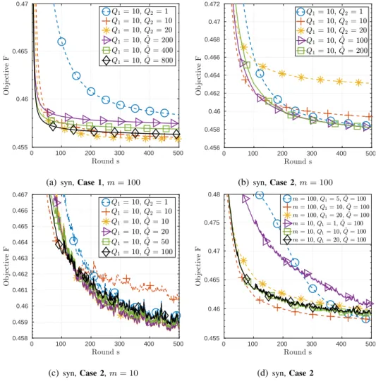
B. Convergence of FedMAvg
In Fig. 1(a) and Fig. 1(b), we present the convergence curves of FedMAvg for Q1 = 10 and for
constantQ2 and diminishingQ2, onCase 1andCase 2of synthetic data, respectively. One can observe
from Fig. 1(a) that for constant Q2, increasing Q2 can speed up the convergence under Case 1 (i.i.d.
data). On the contrary, one can see from Fig. 1(b) that under Case 2(non-i.i.d. data), increasingQ2 can
greatly cause larger floors, whereas, with diminishing Q2, a proper value of Qˆ can not only speed up
the convergence but also achieve a lower objective value. The choice of Qˆ may depend on the dataset.
As shown in [42, Fig. S1(a)], a small value of Qˆ = 5can achieve a good convergence behavior for the
0 100 200 300 400 500 0.455
0.46 0.465 0.47
(a)syn,Case 1,m= 100
0 100 200 300 400 500 0.456 0.458 0.46 0.462 0.464 0.466 0.468 0.47 0.472 (b)syn,Case 2,m= 100 0 100 200 300 400 500 0.458 0.459 0.46 0.461 0.462 0.463 0.464 0.465 0.466 0.467 (c)syn,Case 2,m= 10 0 100 200 300 400 500 0.455 0.46 0.465 0.47 0.475 0.48 (d)syn,Case 2
Fig. 1: Convergence curve versus number of rounds of FedMAvg with different values ofQ1 andQˆ.
Fig. 1(c) considers the PCC scheme withm= 10. By comparing Fig. 1(c) with Fig. 1(b), one can see
that the degradation due to constantQ2becomes more evident when only partial clients communicate with
the server, whereas the diminishingQ2 scheme with a smaller value ofQˆ can converge well. Moreover,
as displayed in Fig. 1(d), increasingQ1 property can also speed up the convergence for both full client
participation and PCC. While Fig. 1(d) is for Case 2, the same trend can be observed for Case 1; see [42, Fig. S1(b)]. The above results well corroborate with Theorem 1.
As discussed in Section III-A, the adopted PCC scheme can yield better performance than the PCP scheme. To verify this, we present in Fig. 2(a) the comparison results of FedMAvg with PCC and PCP, respectively. One can observe that FedMAvg with PCC can significantly outperform that with PCP.
Lastly, we verify the discussion in Remark 1 that the proposed FedMAvg with sequential updating in (11)-(14) is better than the direct application of PALM (15)-(16). In Fig. 2(b), we denote the latter approach as “FedPALM”, and one can clearly see that FedPALM cannot perform well except forQ= 2
0 100 200 300 400 500 0.455 0.46 0.465 0.47 0.475 0.48 0.485 0.49
(a) syn,Case 2,m= 10
0 100 200 300 400 500 0.46 0.47 0.48 0.49 0.5 0.51 (b)syn,Case 1,m= 100
Fig. 2: (a) Comparison between FedMAvg (PCP) and FedMAvg (PCC), and (b) comparison of FedMAvg and naive FedPALM mentioned in Remark 1.
(one step of updates of Wp and Hp per client).
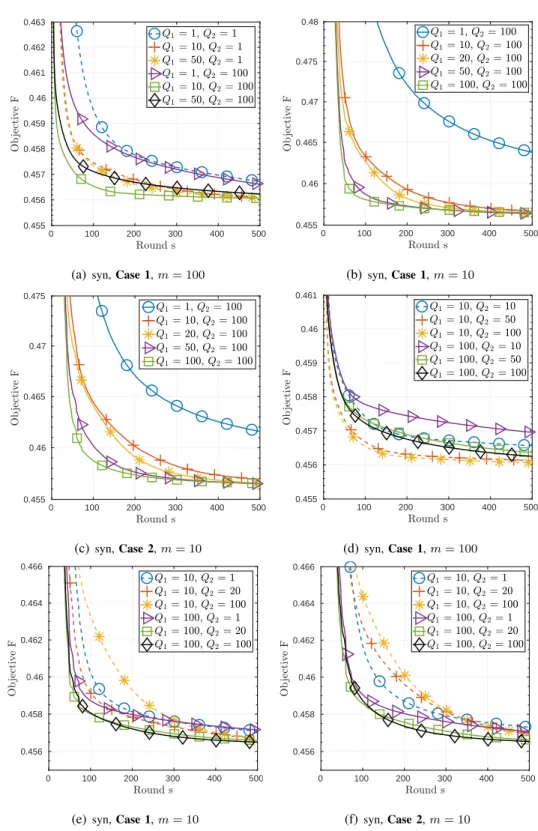
C. Convergence of FedMGS
In Fig. 3, the convergence curves of the FedMGS algorithm on the synthetic dataset are displayed. Fig. 3(a) shows that increasing Q1 can speed up the convergence, but the speedup with Q1 > 10 is not as
significant as that with Q1= 10. One can also see that the method in [13] and [14], which corresponds
to FedMGS withQ1 =Q2 = 1, converges much slower than FedMGS with Q1 >1 andQ2 >1.
As shown in Fig. 3(b), increasingQ1 can monotonically improve the convergence rate whenm= 10;
the same trend is also observed in Fig 3(c) for Case 2 non-i.i.d. data. On the other hand, one can see from Fig. 3(d) that FedMGS with m = 100 (full client participation) and Q1 = 10 or 100 can have
monotonically improved convergence speed when Q2 increases. However, as shown in Fig. 3(e), when
m = 10, increasing Q2 can improve the convergence only if Q1 is also large (Q1 = 100). We remark
that similar insights apply to the Case 2 non-i.i.d data, which are shown in Fig 3(f). In summary, one can conclude that the algorithm convergence can benefit from a largeQ2 and smallQ1 whenm is large
while from both largeQ1 andQ2 when m is small.
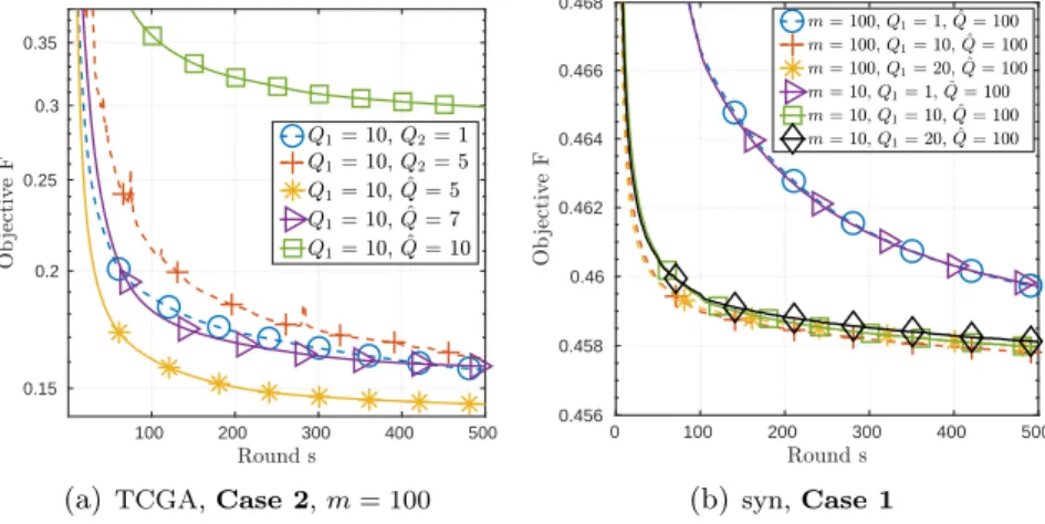
D. Effect of i.i.d and non i.i.d Data
We further examine the performance of FedMAvg and FedMGS when faced with i.i.d (Case 1) and non-iid data (Case 2). One can see from Fig. 4(a) and Fig. 4(c) that data distribution can have a considerable impact on the FedMAvg for both the synthetic and TCGA dataset (also see the results on TDT2 and MNIST datasets in [42, Fig. S2]) although full participation (m= 100) may alleviate the degradation.
0 100 200 300 400 500 0.455 0.456 0.457 0.458 0.459 0.46 0.461 0.462 0.463
(a)syn,Case 1,m= 100
0 100 200 300 400 500 0.455 0.46 0.465 0.47 0.475 0.48 (b)syn,Case 1,m= 10 0 100 200 300 400 500 0.455 0.46 0.465 0.47 0.475 (c)syn,Case 2,m= 10 0 100 200 300 400 500 0.455 0.456 0.457 0.458 0.459 0.46 0.461 (d)syn,Case 1,m= 100 0 100 200 300 400 500 0.456 0.458 0.46 0.462 0.464 0.466
(e) syn,Case 1,m= 10
0 100 200 300 400 500 0.456 0.458 0.46 0.462 0.464 0.466 (f) syn,Case 2,m= 10
Fig. 3: Convergence curve versus number of rounds of FedMGS for different values of Q1 and Q2.
In Fig. 4(b) and Fig. 4(d), the results of FedMGS are shown, and it can be observed that FedMGS is more robust against the data distribution. In particular, when full participation (m= 100), FedMGS can
0 100 200 300 400 500 0.455
0.46 0.465 0.47
(a)FedMAvg, syn
0 100 200 300 400 500 0.455 0.46 0.465 0.47 (b)FedMGS, syn 0 100 200 300 400 500 0.14 0.15 0.16 0.17 0.18 0.19 0.2 (c)FedMAvg, TCGA 0 100 200 300 400 500 0.14 0.15 0.16 0.17 0.18 0.19 0.2 (d)FedMGS, TCGA
Fig. 4: Convergence curve versus number of rounds FedMAvg and FedMGS on the four datasets. It is set thatQ1 = 10for both FedMAvg and FedMGS for all datasets.
FedMGS is equivalent to applying the PALM to problem (2) over the network. E. Comparison between FedMAvg and FedMGS
In Fig. 5, we compare the FedMAvg and FedMGS on the non-i.i.d. synthetic and TCGA dataset (also see the results on TDT2 and MNIST datasets in [42, Fig. S3]). The setting of Q1 and Q2 ( ˆQ) is the
same as that in Section V-D. One can see from Fig. 5(a) and Fig. 5(c) that on the synthetic data FedMGS performs significantly better than FedMAvg for almost all values ofm under test. One can also see that
with increased m both algorithms have improved convergence speed.
Fig. 5(b) and Fig. 5(d) re-plot the same results but with respect to the communication cost. One can see that PCC are quite effective in reducing the communication cost for FedMAvg since a smaller value ofm
0 100 200 300 400 500 0.455
0.46 0.465 0.47
(a)syn,Case 2,F v.s. rounds
0 2 4 6 8 10 108 0.455 0.46 0.465 0.47
(b)syn,Case 2,F v.s. com. cost
0 100 200 300 400 500 0.14 0.15 0.16 0.17 0.18 0.19 0.2
(c)TCGA,Case 2,F v.s. rounds
0 0.5 1 1.5 2 109 0.14 0.15 0.16 0.17 0.18 0.19 0.2
(d)TCGA,Case 2,F v.s. com. cost
Fig. 5: Convergence curve versus number of rounds and communication cost of FedMAvg and FedMGS under non-i.i.d data.
communication costs. The effect of PCP for FedMGS is not that significant because the convergence speed of FedMGS with m = 100 is far faster than that with m <100 on these two dataset. However,
one can see from [42, Fig. S3] that on the MNIST dataset, the FedMGS with m = 10 can save the
communication cost than that with m= 100.
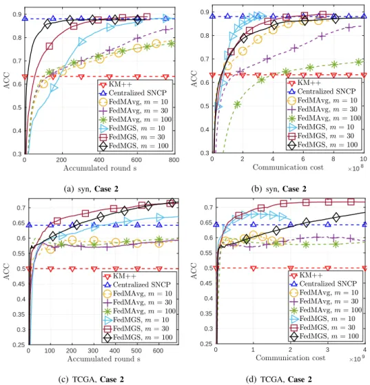
F. Clustering Performance
To evaluating the clustering performance of the proposed algorithms, we follow the successive non-convex penalty (SNCP) approach in [44] to gradually increase the penalty parameterρ in (35) whenever
problem (2) is solved with sufficiently smallε. Specifically, the initialρis set to 10−8 and is updated by ρ= 1.5×ρ wheneverε <1×10⁻⁵ (resp.ε <5×10⁻⁵ ) for FedMAvg (resp. FedMGS). The stopping
0 200 400 600 800 0.3 0.4 0.5 0.6 0.7 0.8 0.9
(a) syn,Case 2
0 2 4 6 8 10 108 0.3 0.4 0.5 0.6 0.7 0.8 0.9 (b)syn,Case 2 0 100 200 300 400 500 600 0.25 0.3 0.35 0.4 0.45 0.5 0.55 0.6 0.65 0.7 (c) TCGA,Case 2 0 1 2 3 4 109 0.25 0.3 0.35 0.4 0.45 0.5 0.55 0.6 0.65 0.7 (d)TCGA,Case 2
Fig. 6: Clustering accuracy versus number of accumulated rounds or communication cost of FedMAvg and FedMGS for different datasets.
addition, the centralized SNCP method [44, Algorithm 1 & 2] and the popular K-means++ [46] are also implemented as two benchmarks.
Fig. 6 presents the clustering accuracy (ACC) [26] versus accumulated round number and communica-tion cost on the synthetic and TCGA datasets (also see the results on TDT2 and MNIST datasets in [42, Fig. S4]). One can observe that FedMGS outperforms FedMAvg and achieves much higher clustering accuracy than K-means++. From Fig. 6(a)-(b), one can see that FedMGS yields comparable clustering accuracy as the centralized SNCP. Surprisingly, one can see from Fig. 6(c)-(d) that FedMGS can even perform better than the centralized SNCP on the TCGA data. More importantly, withm= 10or30, both
of the FedMGS and FedMAvg can quickly reach a higher clustering accuracy with lower communication cost than their counterparts withm= 100.
TABLE I: Clustering accuracy (%) of the considered five methods on the four datasets (Case 2).
Dataset syn TDT2 TCGA MNIST
KM|| 69.4 32.6 50.1 46.8 BEL 38.7 33.3 42.0 46.1 CAL 63.6 32.5 48.2 46.6 FedMAvg (m= 10) 86.2 47.2 58.4 48.8 FedMAvg (m= 100) 85.5 52.1 62.9 40.0 FedMGS (m= 10) 88.4 51.5 67.7 50.0 FedMGS (m= 100) 87.7 53.5 72.2 49.1 75 50 25 0 25 50 75 60 40 20 0 20 40 60 80
(a) Ground truth
75 50 25 0 25 50 75 60 40 20 0 20 40 60 80 (b)KM|| 75 50 25 0 25 50 75 60 40 20 0 20 40 60 80 (c) BEL 75 50 25 0 25 50 75 60 40 20 0 20 40 60 80 (d)CAL 75 50 25 0 25 50 75 60 40 20 0 20 40 60 80 (e)FedMAvg (m= 100) 75 50 25 0 25 50 75 60 40 20 0 20 40 60 80 (f) FedMGS (m= 100)
Fig. 7: Visualized clustering results (by t-SNE [47]) of the considered five methods on the TCGA dataset (Case 2).
G. Comparison with Existing Distributed Clustering Methods
We further examine the clustering performance of the proposed FedMAvg and FedMGS methods against three state-of-the-art distributed clustering methods, including KM|| [33], BEL [37], and CAL [39]. These methods require only few rounds of communications between the clients and the server. For example, both of BEL and CAL need merely one round of communication to obtain the clustering results. The distributed version of KM|| is similar to the parallel counterpart of the K-means++ which requires few communication rounds as well.
Table I shows the detailed clustering accuracy of all methods on the four datasets underCase 2over 100 clients. Note that the parameter settings of FedMAvg and FedMGS are the same as those in Section V-F. As seen in Table I, the proposed FedMGS achieves the highest clustering accuracy. Besides, although FedMAvg provides worse performance than FedMGS, it still outperforms the other three distributed clustering methods considerably. Fig. 7 presents the visualized clustering results (by t-SNE [47]) of all methods on the TCGA dataset underCase 2. One can see that both of the FedMAvg and FedMGS greatly outperform the other three distributed counterparts.
VI. CONCLUSION
In this paper, we have presented FedMAvg and FedMGS algorithms for FedMF problems and con-sidered their application to the fundamental data clustering task. We have also provided theoretical convergence analyses for the two algorithms. The analysis results have explicitly characterized the impacts of non-i.i.d. data, partial client communication as well as local GD number on the convergence of of the two algorithms. They have also suggested a diminishing Q2 strategy for FedMAvg to deal with the
non-i.i.d. data, and also imply that FedMGS is less sensitive to data distribution. Extensive experiment results have demonstrated consistent convergence behaviors of the proposed algorithms on both synthetic and real datasets, showing insights on the values ofQ1 andQ2 ( ˆQ) that can improve the convergence speed
of both algorithms. It has also been shown that PCC/PCP can significantly reduce the communication cost of both algorithms.
As the future works, it is worthwhile to devise FedMF algorithms for general MF models that can handle outlier and noisy data [48] as well as considering other MF applications, such as item recommendation and biological data analysis. Enhancing privacy and security [14] of FedMF algorithms is also of great importance. APPENDIXA PROOF OFTHEOREM1 According to (20), we define f Ws,t=PW(Ws,t), Ws,t= 1 m X p∈As Wps,t, (37)
for all sand t={0} ∪ Q1∪ Qs2. Then, by (12), we have
f
We also define Es−1 ={A1, . . . ,As−1,{H1,t}Qt=01 , . . . ,{Hs−1,t}Qt=0s−1, {W1,t}Qt=01 , . . . ,{Ws−1,t} Qs−1 t=0 , {c1p}Pp=1, . . . ,{cps−1}Pp=1, d1, . . . , ds−1} (39)
as the collection of historical events up to round(s−1).
Objective Descent w.r.t. H: According to [40, Lemma 3.2], (11), (12) and (38) imply
Fp(Wfs,t,Hs,tp )−Fp(Wfs,t−1,Hs,tp −1)
≤ −γ12−1LHkHs,tp −1−Hs,tp k2F,∀t∈ Q1, (40)
since cs
p = γ1L2H. Summing up (40) from t= 1 to Q1 and taking expectation of it conditional on Es−1
yields E[Fp(Wfs,Q1,Hs,Qp 1)|Es−1]−E[Fp(Wfs,0,Hs,0p )|Es−1] ≤ − γ1−1 2 Q1 X t=1 LHE[kHs,tp −1−Hs,tp k2F|Es−1]. (41)
As a result, the objective function F descends with local updates ofH as follows
E[F(Wfs,Q1,Hs,Q1)|Es−1]−E[F(Wfs,0,Hs,0)|Es−1] ≤ − γ12−1 Q1 X t=1 P X p=1 ωpLHE[kHs,tp −1−Hs,tp k2F|Es−1]. (42) Objective Descent w.r.t. W: Note by (13) that Hs,tp = Hs,tp −1,∀t ∈ Qs2. Since ∇WF(·,Hs,Q) is
Lipschitz continuous under Assumption 2, by the descent lemma [40, Lemma 3.1], we have
F(Wfs,t,Hs,t)≤F(Wfs,t−1,Hs,t−1) +L s W 2 kWf s,t−Wfs,t−1k2 F +h∇WF(Wfs,t−1,Hs,t−1),Wfs,t−Wfs,t−1i | {z } ,(a) . (43)
The term (a)can be bounded by the following lemma which is proved in [42, Section 1.1].
Lemma 1 For any sandt∈ Qs
h∇WF(Wfs,t−1,Hs,t−1),Wfs,t−Wfs,t−1i ≤ −dskWfs,t−Wfs,t−1k2F + ∇WF(Wfs,t−1,Hs,t−1)− 1 m X p∈As ∇WFp(Ws,tp −1,Hps,t−1),Wfs,t−Wfs,t−1 . (44)
Thus, substituting (44) into (43) gives rise to
F(Wfs,t,Hs,t) ≤F(Wfs,t−1,Hs,t−1)− ds−L s W 2 kWfs,t−Wfs,t−1k2F + ∇WF(Wfs,t−1,Hs,t−1)− 1 m X p∈As ∇WFp(Ws,tp −1,Hps,t−1),Wfs,t−Wfs,t−1 ≤F(Wfs,t−1,Hs,t−1)− d s−Ls W 2 kWf s,t−Wfs,t−1k2 F + 1 2ds ∇WF(Wfs,t−1,Hs,t−1)− 1 m X p∈As ∇WFp(Wps,t−1,Hs,tp −1) 2 F , (45)
where (45) holds since hx,yi ≤ 2c1kxk2
2 + c2kyk22,∀c > 0. Then, taking the expectation over the two
sides of (45) conditioned on Es−1 yields
E[F(Wfs,t,Hs,t)|Es−1]−E[F(Wfs,t−1,Hs,t−1)|Es−1] ≤ −E ds−LsW 2 kWf s,t−Wfs,t−1k2 F Es−1 + 1 2dsE ∇WF(Wfs,t−1,Hs,t−1)− 1 m X p∈As ∇WFp(Wps,t−1,Hs,tp −1) 2 F Es−1 . (46)
We then proceed with the following lemma which is proved in [42, Section 1.2].
Lemma 2 For any sandt∈ Qs
2, E∇WF(Wfs,t−1,Hs,t−1) − 1 m X p∈As ∇WFp(Wps,t−1,Hs,tp −1) 2 F Es−1 ≤ 2 +16 m XP p=1 ωp(LsWp) 2E[kWfs,t−1−Ws,t−1 p k2F|Es−1] + 16 mζ 2.
By applying Lemma 2, we have E[F(Wfs,t,Hs,t)|Es−1]−E[F(Wfs,t−1,Hs,t−1)|Es−1] ≤ −E ds−LsW 2 kWf s,t−Wfs,t−1k2 F Es−1 + 1 + 8/m ds XP p=1 ωp(LsWp) 2E[kWfs,t−1−Ws,t−1 p k2F|Es−1] + 8ζ2 mds, ∀t∈ Q s 2. (47)
Summing (47) up from t=Q1+ 1to Qs yields
E[F(Wfs,Qs,Hs,Qs)|Es−1]−E[F(Wfs,Q1,Hs,Q1) |Es−1] ≤ − ds −Ls W 2 E Qs X t=Q1+1 kWfs,t−Wfs,t−1k2F Es−1 +8Q s 2ζ2 mds +1 + 8/m ds Qs X t=Q1+1 P X p=1 ωp(LsWp) 2E[ kWfs,t−1−Wps,t−1k2F|Es−1] | {z } ,(b) . (48)
The term (b) can be bounded with the following lemma which is proved in [42, Section 1.3].
Lemma 3 Let γ2≥Qs2 q 2(7 + 4L2W/L2W). It holds that Qs X t=Q1+1 P X p=1 ωp(LsWp) 2E[kWfs,t−1−Ws,t−1 p k2F|Es−1] ≤2C s 1(11ζ 2 3 +φ2) γ2 2 , (49) whereC1s,Qs2(Qs2−1)(2Qs2−1). Sinceγ2= max{Q12 q 2(7 + 4L2W/L2W),√T}andQs2=bQsˆc+ 1, we haveγ2 ≥Qs2 q 2(7 + 4L2W/L2W). Thus, (48) becomes E[F(Wfs,Qs,Hs,Qs)|Es−1]−E[F(Wfs,Q1,Hs,Q1)|Es−1] ≤ − ds−LsW 2 Qs X t=Q1+1 E[kWfs,t−Wfs,t−1k2F|Es−1] +2(1 + 8/m)( 11ζ2 3 +φ2)C1s dsγ2 2 +8Q s 2ζ2 mds (50) ≤ − γ2−1 2 Qs X t=Q1+1 LsWE[kWfs,t−Wfs,t−1k2F|Es−1] + 2(1 + 8/m)(11ζ32 +φ2)C1s γ3 2LsW + 8Q s 2ζ2 mγ2LsW , (51)
where (51) follows sinceds=γ
2LsW. Then combing (42) and (51) and taking expectation over two sides
yields γ1−1 2 Q1 X t=1 P X p=1 ωpLHE[kHps,t−1−Hs,tp k2F] +γ2−1 2 Qs X t=Q1+1 LsWE[kWfs,t−Wfs,t−1k2F] ≤E[F(Wfs,0,Hs,0)]−E[F(Wfs,Qs,Hs,Qs)] +2(1 + 8/m)( 11ζ2 3 +φ2)C1s γ23LsW + 8Qs2ζ2 mγ2LsW . (52)
Derivation of the Main Result:We next derive the convergence in terms of the optimal gap functions
in (21) and (22). Since csp= γ1LH
2 , we have from (52) that Q1 X t=1 E[GH(Wfs,t−1,Hs,t−1)] = Q1 X t=1 P X p=1 ωp(csp)2E[kHps,t−1−Hs,tp k2F] ≤ γ 2 1LH 2(γ1−1) E[F(Wfs,0,Hs,0)]−E[F(Wfs,Qs,Hs,Qs)] +(1 + 8/m)( 11ζ2 3 +φ2)C1sγ21LH γ3 2(γ1−1)LsW + 4Q s 2ζ2γ12LH mγ2(γ1−1)LsW , (53)
Then, summing (53) up from s= 1 to S yields
S X s=1 Q1 X t=1 E[GH(Wfs,t−1,Hs,t−1)] ≤ γ 2 1LH 2(γ1−1) F(Wf1,0,H1,0)−F +4ζ 2γ2 1LHPSs=1Qs2 mγ2(γ1−1)LW + (1 + 8/m)( 11 3ζ2+φ2)γ12LHPSs=1C1s γ3 2(γ1−1)LW . (54)
where (54) follows from (17).
S X s=1 Qs X t=Q1+1 E[kWfs,t−Wfs,t−1k2F] ≤ 2 (γ2−1)LW F(Wf1,0,H1,0)−E[F(WfS+1,0,HS+1,0)] + S X s=1 E 4(1 + 8/m)(11ζ2 3 +φ2)C1s γ23(γ2−1)(LsW)2 + 16Q s 2ζ2 mγ2(γ2−1)(LsW)2 ≤(γ 2 2−1)LW F(Wf1,0,H1,0)−F + 16ζ 2PS s=1Qs2 mγ2(γ2−1)L2W +4(1 + 8/m)( 11ζ2 3 +φ2) PS s=1C1s γ3 2(γ2−1)L2W . (55)
Then, we need the following lemma to bound the optimality gap GW(Wfs,t,Hs,t), which is proved in
[42, Section 1.5].
Lemma 4 For |As|< P, we have S X s=1 Qs X t=Q1+1 E[GW(Wfs−1,t,Hs−1,t)] ≤3(γ22+ 2)L2W S X s=1 Qs X t=Q1+1 E[kWfs,t−Wfs,t−1k2F] +( 11 3 ζ2+φ2) PS s=1C2s γ2 2 +3(ζ 2+φ2)PS s=1C1s 2 + 96ζ2 m S X s=1 Qs2, whereCs 2 ,6(3Qs2(Qs2−1)/2 + 4 + 32/m)C1s.
By applying Lemma 4, we obtain
S X s=1 Qs X t=Q1+1 E[GW(Wfs,t−1,Hs,t−1)] ≤3(γ22+ 2)L2W 2 (γ2−1)LW F(Wf1,0,H1,0)−F +4(1 + 8/m)( 11 3ζ2+φ2) PS s=1C1s γ23(γ2−1)L2W + 16ζ 2PS s=1Qs2 mγ2(γ2−1)L2W +( 11 3ζ2+φ2) PS s=1C2s γ22 + 3(ζ2+φ2)PSs=1C1s 2 + 96ζ2 m S X s=1 Qs2
≤6(γ 2 2 + 2)L 2 W (γ2−1)LW F(Wf1,0,H1,0)−F +12(γ 2 2+ 2)(1 + 8/m)(113 ζ2+φ2)L 2 W PS s=1C1s γ23(γ2−1)L2W +48(γ 2 2+ 2)ζ2L 2 W PS s=1Qs2 mγ2(γ2−1)L2W +( 11 3ζ2+φ2) PS s=1C2s γ22 + 3(ζ2+φ2)PSs=1C1s 2 + 96ζ2 m S X s=1 Qs2. (56)
Combing (54) and (56) and dividing two sides of it by T =PSs=1Qs=SQ1+PSs=1Qs2 yields
1 T XS s=1 Q1 X t=1 E[GH(Wfs,t−1,Hs,t−1)] + S X s=1 Qs X t=Q1+1 E[GW(Wfs,t−1,Hs,t−1)] ≤ γ12LH 2(γ1−1) +6(γ 2 2+ 1)L 2 W (γ2−1)LW 1 T F(Wf1,0,H1,0)−F +2(1 + 8/m)( 11 3ζ2+φ2) PS s=1C1s T γ3 2LW +8ζ 2PS s=1Qs2 T mγ2LW +( 11 3ζ2+φ2) PS s=1C2s T γ22 + 3(ζ2+φ2)PSs=1C1s 2T + 96ζ2 m PS s=1Qs2 T ≤D T F(Wf1,0,H1,0)−F + 8Dζ 2 mγ2LW +96ζ 2 m +2D(1 + 8/m)( 11 3ζ2+φ2) PS s=1C1s T γ3 2LW +( 11 3ζ2+φ2) PS s=1C2s T γ22 + 3(ζ2+φ2)PSs=1C1s 2T , (57) whereD, γ12LH 2(γ1−1)+ 6(γ2 2+1)L 2 W
(γ2−1)LW , and the 2nd and 3rd terms in the right hand side of (57) follow because
PS
s=1Qs2/T ≤1. This completes the poof.
REFERENCES
[1] F. Pompili, N. Gillis, P. A. Absil, and F. Glineur, “Two algorithms for orthogonal non-negative matrix factorization with application to clustering,”Neurocomputing, vol. 141, no. 2, pp. 15–25, Oct. 2014.
[2] Y. Koren, R. Bell, and C. Volinsky, “Matrix factorization techniques for recommender systems,”Computer, vol. 42, no. 8, pp. 30–37, Aug. 2009.
[3] K. Devarajan, “Non-negative matrix factorization: An analytical and interpretive tool in computational biology,” PLoS Computational Biology, vol. 4, no. 7, pp. 1–12, Jul. 2008.
[4] J. Yin, L. Gao, and Z. Zhang, “Scalable distributed nonnegative matrix factorization with block-wise updates,”IEEE Trans. Knowl. Data Eng., vol. 30, no. 6, pp. 1136–1149, Jun. 2018.
[5] Q. Yang, Y. Liu, T. Chen, and Y. Tong, “Federated machine learning: Concept and applications,”ACM Transactions on Intelligent Systems and Technology, vol. 10, no. 2, pp. 1–19, Jan. 2019.
[6] J. Kˇonecn´y, H. B. McMahan, D. Ramage, and P. Richtarik, “Federated optimization: Distributed machine learning for on-device intelligence,”arXiv preprint arXiv:1610.02527, 2016.
[7] T.-H. Chang, M. Hong, H.-T. Wai, X. Zhang, and S. Lu, “Distributed learning in the nonconvex world: From batch data to streaming and beyond,”IEEE Signal Process. Mag., vol. 37, no. 3, pp. 26–38, May 2020.
[8] H. B. McMahan, E. Moore, D. Ramage, S. Hampson, and B. A. Areas, “Communication-efficient learning of deep networks from decentralized data,” inProc. ICML, Sydney, Australia, Aug. 6-11, 2017, pp. 1–10.
[9] T. Li, A. K. Sahu, M. Sanjabi, M. Zaheer, A. Talwalkar, and V. Smith, “Federated optimization in heterogeneous networks,” in Proc. MLSys, Austin, TX, USA, Mar. 2-4, 2020, pp. 1–12.
[10] M. Kamp, L. Adilova, J. Sicking, F. Huger, P. Schlicht, T. Wirtz, and S. Wrobel, “Efficient decentralized deep learning by dynamic model averaging,” inProc. ECML PKDD, Dublin, Ireland, Sept. 10-14, 2018, pp. 393–409.
[11] H. Yu, S. Yang, and S. Zhu, “Parallel restarted SGD with faster convergence and less communication: Demystifying why model averaging works,” inProc. AAAI, Honolulu, Hawaii, USA, Jan. 27-Feb. 1, 2019, pp. 5693–5700.
[12] X. Li, K. Huang, W. Yang, S. Wang, and Z. Zhang, “On the convergence of FedAvg on non-iid data,” inProc. ICLR, Addis Ababa, ETHIOPIA, Apr. 26 - May 1, 2020, pp. 1–11.
[13] I. Heged˝us, G. Danner, and M. Jelasity, “Decentralized recommendation based on matrix factorization: A comparison of gossip and federated learning,” inProc. ECML PKDD, W¨urzburg, Germany, Sep. 16-20, 2019, pp. 317–322.
[14] D. Chai, L. Wang, K. Chen, and Q. Yang, “Secure federated matrix factorization,”IEEE Intelligent Systems, vol. 1, No. 1, pp. 1–8, Aug. 2020.
[15] R. Gemulla, E. Nijkamp, R. J. Haas, and Y. Sismanis, “Large-scale matrix factorization with distributed stochastic gradient descent,” inProc. KDD, San Diego, CA, USA, Aug. 21-24, 2011, pp. 69–77.
[16] S. Schelter, C. Boden, M. Schenck, A. Alexandrov, and V. Markl, “Distributed matrix factorization with MapReduce using a series of broadcast-joins,” inProc. RecSys, Hong Kong, China, Oct. 12-16, 2013, pp. 281–284.
[17] F. Li, B. Wu, L. Xu, C. Shi, and J. Shi, “A fast distributed stochastic gradient descent algorithm for matrix factorization,” in Proc. BIGMINE, New York, USA, Aug. 24, 2014, pp. 77–87.
[18] S. Schelter, V. Satuluri, and R. B. Zadeh, “Factorbird-A parameter server approach to distributed matrix factorization,”
arXiv preprint arXiv:1411.0602, 2019.
[19] C. Liu, H.-C. Yang, J. Fan, L.-W. He, and Y.-M. Wang, “Distributed nonnegative matrix factorization for web-scale dyadic data analysis on MapReduce,” inProc. WWW, Raleigh, USA, Apr. 26-30, 2010, pp. 681–190.
[20] R. Zdunek and K. Fonal, “Distributed nonnegative matrix factorization with HALS algorithm on MapReduce,” in
International Conference on Algorithms and Architectures for Parallel Processing, Helsinki, Finland, Aug. 21-23, 2017, pp. 211–222.
[21] H.-T. Wai, T.-H. Chang, and A. Scaglione, “A consensus-based decentralized algorithm for non-convex optimization with application to dictionary learning,” inProc. IEEE ICASSP, Brisbane, QLD, Australia, Apr. 19-24, 2015, pp. 3546–3550. [22] M. Hong, D. Hajinezhad, and M.-M. Zhao, “Prox-PDA: The proximal primal-dual algorithm for fast distributed nonconvex
optimization and learning over networks,” inProc. ICML, Sydney, Australia, Aug. 6-11, 2017, pp. 1529–1538.
[23] C. Chen, Z. Liu, P. Zhao, J. Zhou, and X. Li, “Privacy preserving point-of-interest recommendation using decentralized matrix factorization,” inProc. AAAI, Louisiana, USA, Feb. 2-7, 2018, pp. 257–264.
[24] Z. Zhu, Q. Li, X. Yang, G. Tang, and M. B. Wakin, “Distributed low-rank matrix factorization with exact consensus,” in
[25] M. Udell, C. Horn, R. Zadeh, and S. Boyd, “Generalized low rank models,”Foundations and Trends in Machine Learning, vol. 9, no. 1, pp. 1–118, Aug. 2009.
[26] D. Cai, X. He, and J. Han, “Locally consistent concept factorization for document clustering,”IEEE Trans. Knowl. Data Eng., vol. 23, no. 6, pp. 902–913, Jun. 2011.
[27] R. Mclendon, A. Friedman, D. Bigneret al., “Comprehensive genomic characterization defines human glioblastoma genes and core pathways,”Nature, vol. 455, no. 7216, pp. 1061–1068, Oct. 2008.
[28] Y. LeCun, C. Cortes, and C. Burges. The mnist database. [Online]. Available: http://yann.lecun.com/exdb/mnist/
[29] J. Kˇonecn´y, H. B. McMahan, and D. Ramage, “Federated optimization: Distributed optimization beyond the datacenter,” in NeuIPS Optimization for Machine Learning Workshop, Montreal, Quebec, Canada, Dec. 7-12, 2015, pp. 1–5. [30] C. Bauckhage, “K-means clustering is matrix factorization,”arXiv preprint arXiv:1512.07548, 2015.
[31] S. Wang, T.-H. Chang, Y. Cui, and J.-S. Pang, “Clustering by orthogonal non-negative matrix factorization: A sequential non-convex penalty approach,” inProc. IEEE ICASSP, Brighton, UK, May 12-17, 2019, pp. 5576–5580.
[32] I. S. Dhillon and D. S. Modha, “A data-clustering algorithm on distributed memory multiprocessor,” inLarge-Scale Parallel Data Mining, Springer-Verlag London, UK, Jul. 19999, pp. 245–260.
[33] B. Bahmani, B. Moseley, A. Vattani, R. Kumar, and S. Vassilvitskii, “Scalable K-means++,” in Proc. VLDB, Istanbul, Turkey, Aug. 27-31, 2012, pp. 622–633.
[34] T. Kucukyilmaz, “Parallel K-Means algorithm for shared memory multiprocessors,”Journal of Computer and Communi-cations, vol. 2, no. 11, pp. 15–23, Jan. 2014.
[35] M. Ester, H. P. Kriegel, J. Sander, and X. Xu, “A density-based algorithm for discovering clusters in large spatial databases with noise,” inProc. KDD, Portand, Oregon, USA, Aug. 1996, pp. 226–231.
[36] H. Ding, Y. Liu, L. Huang, and J. Li, “K-means clustering with distributed dimensions,” inProc. ICML, New York, NY, USA, Jun. 19-24, 2016, pp. 1339–1348.
[37] M.-F. Balcan, S. Ehrlich, and Y. Liang, “Distributed k-means and k-median clustering on general topologies,” inProc. NeuIPS, Lake Tahoe, USA, Dec. 5-10, 2013, pp. 1995–2003.
[38] X. Guo and S. Li, “Distributed k-clustering for data with heavy noise,” inProc. NeuIPS, Montreal, Quebec, Canada, Dec. 2-8, 2018, pp. 7849–7857.
[39] J. Chen, E. S. Azer, and Q. Zhang, “A practical algorithm for distributed clustering and outlier detection,” inProc. NeuIPS, Montreal, Quebec, Canada, Dec. 2-8, 2018, pp. 2248–2256.
[40] J. Bolte, S. Sabach, and M. Teboulle, “Proximal alternating linearized minimization for non-convex and non-smooth problems,” Math Program., vol. 146, no. 1, pp. 459–494, Aug. 2014.
[41] X. Lian, C. Zhang, H. Zhang, C.-J. Hsieh, W. Zhang, and J. Liu, “Can decentralized algorithms outperform centralized algorithms? A case study for decentralized parallel stochastic gradient descent,” inProc. NeuIPS, California, USA, Dec. 4-9, 2017, p. 5336–5346.
[42] S. Wang and T.-H. Chang, “Supplementary material of Federated matrix factorization: Algorithm design and application to data clustering.” [Online]. Available: https://arxiv.org/abs/2002.04930
[43] C. Fevotte and J. Idier, “Algorithms for nonnegative matrix factorization with theβ-divergence,”Neural Computation, vol.
23, no. 9, pp. 2421–2456, Sept. 2011.
[44] S. Wang, T.-H. Chang, Y. Cui, and J.-S. Pang, “Clustering by orthogonal NMF model and non-convex penalty optimization,”
arXiv preprint arXiv:1906.00570, 2019.
[45] B. Yang, X. Fu, and N. D. Sidiropoulos, “Learning from hidden traits: Joint factor analysis and latent clustering,”IEEE Trans. Signal Process., vol. 65, no. 1, pp. 256–269, Jan. 2017.
[46] D. Arthur and S. Vassilvitskii, “K-means++: The advantages of careful seeding,” inProc. SODA, Philadelphia, PA, USA, Jan. 7-8, 2007, pp. 1027–1035.
[47] L. V. D. Maaten and G. E. Hinton, “Visualizing data using t-SNE,”JMLR, vol. 9, no. 86, pp. 2579–2605, Dec. 2008. [48] L. Mackey, A. Talwalkar, and M. I. Jordan, “Distributed matrix completion and robust factorization,”JMLR, vol. 16, no. 28,
1
Proofs of Lemmas for Theorem 1
1.1 Proof of Lemma 1
Firstly, by (13) and (37), we have
0 = 1 m X p∈As ∇WFp(Ws,tp −1,Hs,tp −1) +ds(W s,t −Ws,t−1). (S.1)
Secondly, consider the following term
h∇WF(Wfs,t−1,Hs,t−1) +ds(Wfs,t−Wfs,t−1),Wfs,t−1−Wfs,ti = ∇WF(Wfs,t−1,Hs,t−1) +ds(Wfs,t−Wfs,t−1) − 1 m X p∈As ∇WFp(Ws,tp −1,Hs,tp −1)−ds(W s,t −Ws,t−1),Wfs,t−1−Wfs,t (S.2) = ∇WF(Wfs,t−1,Hs,t−1)− 1 m X p∈As ∇WFp(Wfps,t−1,Hps,t−1),Wfs,t−1−Wfs,t +dshWfs,t−Ws,t,Wfs,t−1−Wfs,ti+dshWfs,t−1−Ws,t−1,Wfs,t−Wfs,t−1i ≥ ∇WF(Wfs,t−1,Hs,t−1)− 1 m X p∈As ωp∇WFp(Wfs,tp −1,Hs,tp −1),Wfs,t−1−Wfs,t , (S.3)
where (S.2) holds due to (S.1), and (S.3) follows because
hWfs,t−Ws,t,Wfs,t−1−Wfs,ti ≥0,
hWfs,t−1−Ws,t−1,Wfs,t−Wfs,t−1i ≥0. (S.4) Inequalities in (S.4) are obtained by the fact that Wfs,t=PW{Ws,t} and Wfs,t−1 =PW{Ws,t−1}, and the application of the optimality condition hx? −z,x−x?i ≥ 0,∀x ∈ X of the projection
problemx? = arg min
x∈X
1
2kx−zk22, whereX is a closed convex set [?, Proposition 3.1.1]. Rearranging
the terms in (S.3) yields
h∇WF(Wfs,t−1,Hs,t−1),Wfs,t−Wfs,t−1i ≤ −dskWfs,t−Wfs,t−1k2F + ∇WF(Wfs,t−1,Hs,t−1)− 1 m X p∈As ∇WFp(Ws,tp −1,Hps,t−1),Wfs,t−Wfs,t−1 . (S.5) 1