An investigation of bio potentials for the pre-diagnosis of heart dysfunction using a novel portable high resolution electronic analyzer and software

«An investigation of bio potentials for the pre-diagnosis of heart

dysfunction using a novel portable high resolution electronic

analyzer and software»

Thesis submitted to the Faculty of Computing, Engineering & Technology of Staffordshire University in partial fulfillment of the requirements for the degree

Doctor of Philosophy

Author: ANDONOPOULOS JOHN

Supervised by:

Prof. Noel Shammas

Prof. Steve Grainger

Dr. Ian Taylor

Prof. Theodore Ganetsos

Antonopoulos John – PHD Research Page 3

I. Acknowledgments

Completing a PhD is truly a marathon event, and I would not have been able to complete this journey without the aid and support of many people over the past four years. I must first express my gratitude towards my principal supervisor, Professor Noel YA Shammas whose expertise, understanding, and patience, added considerably to my research experience.

I would like to thank the other members of my committee, Dr Ian Taylor, and Prof. Steve Grainger for the assistance they provided at all levels of the research project.

I want to express my gratitude to Dr. Theodore Ganetsos, for his supervision, advice, and guidance from the very early stage of this research. He provided me with direction, technical support and became more of a mentor and friend, than a professor. I am indebted to him more than he knows.

In addition, I want to thank my friend and associate Nikolaos Laskaris for his advice, and crucial contribution, which made him a backbone of this research and so to this research. Also I would like to thank my friend Anastasios Arvanitis for his assistance to the research editing.

I gratefully thank Mrs Tracy Davies for her continuous support through all these years.

Finally, I would also like to thank my family for the support they provided me through my entire life and in particular, I must acknowledge my wife and best friend, Sofia, without whose love, encouragement and editing assistance, I would not have finished this research.

Antonopoulos John – PHD Research Page 4

II. Abstract

An electrocardiogram (ECG) is a bioelectrical signal which records the heart‘s electrical activity versus time. It is an important diagnostic tool for assessing heart functions. The interpretation of ECG signal is an application of pattern recognition. The techniques used in this pattern recognition comprise: signal pre-processing, QRS detection, creation of variables and signal classification. In this research, signal processing and programs implementation are based in Matlab environment. The processed simulated signal source came from the SIMULAIDS® interactive ECG simulator™ device and the actual heart signals came from actual patients that suffer from various heart disorders, as well as healthy persons that hadn‘t recorded any form of heart condition in the past.

For the creation of the database in this research, 5 types of ECG waveform were selected from the ECG simulator device. These are normal sinus rhythm (NSR), ventricular tachycardia (VT poly), ventricular fibrillation (VF), Atrial fibrillation (A FIB) and supra ventricular tachycardia (SVT). An essential part of this research was the development of a portable high resolution ECG device, capable of connecting with, either an ECG simulator device, or recording real human data. This device is able to produce higher resolution than normal ECG devices and high values of Signal to Noise Ratio (SNR).

Matlab was used to develop a program that could further examine, analyze and study the ECG samples. Since the heart waveform can be simulated by cubic spline interpolation, this feature was used by the implemented Matlab program. The ECG samples were normalized and processed to produce 4 specific coefficients. These 4 coefficients of cubic spline were used in the applied methodology in order to evaluate and separate the various heart disorders with mathematical terms and equations. The database created was compared with the real human samples that were taken and passed through the same data process. Through this step, the entire data process and implementation was not only confirmed, but also proved that the capability to diagnose heart disorders was possible.

Based on the results of the applied methodology, the categorization of heart disorders without actual clinical examination is possible. Further analysis of each group of results, can lead to heart disorder prediction. Also given are further suggestions to plan experiments for future work.

Antonopoulos John – PHD Research Page 6

Table of contents ... 6

List of figures ... 8

List of tables ... 9

List of abbreviations and acronyms ... 10

Chapter 1: Introduction ... 12

1.1. Aims of investigation ... 12

1.2. Project Objectives ... 13

1.3. Summary ... 14

Chapter 2: Literature Survey ... 15

2.1. The Heart ... 15

2.1.1. Bioelectricity of the heart ... 17

2.1.2. Body surface potentials and Electrocardiogram ... 21

2.1.3. Electrophysiology ... 23

2.1.3.1. Electrophysiology of the Heart ... 24

2.1.3.2. The Action Potential of the Single Cell of Working Myocardium ... 25

2.1.3.3. Excitation Propagation and Cardiac Contractions ... 27

2.1.3.4. The Generation of an Electrocardiogram and the Dominant Cardiac Vector ... 29

2.2. Cardiovascular variability signals ... 30

2.2.1. Changes of signal variability connected to specific diseases ... 32

2.2.2. Other events modifying signal variability ... 34

2.2.3. RR interval time series ... 35

2.2.4. ECG waveform detection ... 37

2.2.5. Ambulatory HRV data ... 39

2.2.5.1. Accuracy of HRV measurement ... 40

2.2.5.2. Reproducibility of HRV measurements ... 40

2.2.5.3. Artifacts in RR interval time series ... 42

2.2.5.4. Errors in the detection and classification of QRS complexes ... 43

2.2.5.5. Non-periodic changes in RR intervals ... 46

2.2.5.6. Limitations and effects of artifacts... 47

2.2.5.7. Correction of abnormal RR intervals ... 48

2.2.5.8. Detection of artifacts ... 49

Chapter 3: Analysis of heart signal variability ... 52

3.1. Interpolation of ECG signal ... 52

3.2. Time domain analysis and indices ... 54

3.3. Analysis of distribution ... 54

3.4. Frequency domain analysis ... 55

3.4.1. On the use of spectral analysis ... 57

3.4.2. Mathematical background to spectral analysis ... 58

3.4.3. Spectrum estimation using a periodogram ... 60

3.5. Parametric modeling of time series ... 61

3.6. Estimation of the powers related to components ... 63

3.7. Time frequency analysis ... 66

3.8. Time-variant spectral analysis ... 67

3.9. Wavelet analysis ... 68

3.9.1. Continuous wavelet transform ... 69

3.9.2. Discrete wavelet transform ... 71

3.9.3. Multiresolution wavelet analysis ... 72

3.9.4. Sub band filtering ... 73

3.9.5. Wavelet packet analysis ... 75

3.9.6. Optimization of the wavelet packet decomposition ... 76

3.10. ECG signal preconditioning ... 77

3.11. Non-linear and scale-invariant analysis of the Heart rate ... 85

3.11.1. Scale-independent measures ... 85

Antonopoulos John – PHD Research Page 7

3.12.3. Atrial Arrhythmia ... 95

3.12.3.1. Atrial Tachycardia ... 95

3.12.3.2. Atrial Flutter and Atrial Fibrillation ... 95

3.12.4. Ventricular Arrhythmia ... 96

3.12.4.1. Ventricular Tachycardia... 96

3.12.4.2. Ventricular Flutter ... 97

3.12.4.3. Ventricular Fibrillation ... 98

3.12.5. Wolff - Parkinson - White syndrome ... 98

3.12.6. Heart Conduction Blocks... 99

3.13. Heartbeat Morphologies ... 99

3.13.1. Ischemic Heart Disease ... 99

3.13.2. Myocardial Infarction ... 100

3.13.3. Long QT Syndromes ... 100

3.13.4. Brugada Syndrome ... 102

3.13.5. T-Wave Alternans ... 102

3.14. Torsade de Pointes ... 104

Chapter 4: Methods of investigation... 109

4.1. ECG hardware ... 109

4.1.1. ECG ... 109

4.1.2. Signal processing ... 110

4.1.3. Instrumentation amplifier ... 112

4.1.4. Components and construction ... 113

4.2. Matlab as a tool for creating new ECG analysis program ... 114

4.3. New functions created for this research (to read files ECG of ECG hardware) ... 115

4.4. Cubic Splices ... 120

4.4.1. Basic Features ... 121

4.4.2. Piecewise Polynomials ... 121

4.5. Routine creation ... 125

4.6. Acquisition ... 127

4.6.1. Usual difficulties during the procedure ... 128

4.6.2. Factors that influenced the readings and ways of confrontation ... 129

Chapter 5: Simulation techniques ... 131

5.1. Simulating device ... 131

5.2. Simulated signals ... 133

5.3. Heart rhythm estimation ... 137

5.4. Heart rhythm disorders ... 138

5.5.Real Heart Signals ... 142

5.6. Differences between the theoretical model and various others ... 146

Chapter 6: Conclusions and further development of the research ... 150

6.1. Conclusions ... 150 6.2. Further development ... 151 References ... 153 List of publications ... 164 Appendices ... 165 1. Circuit structure ... 165

2. Changes in the Third Edition of MATLAB ... 166

2.1. The advantages of MATLAB for technical programming ... 166

2.2. Disadvantages of MATLAB ... 167

2.3. How a graphical user interface works ... 168

Antonopoulos John – PHD Research Page 8

Figure 1. Heart and Lungs ... 15

Figure 2. Heart as a main pump of cardiovascular system ... 16

Figure 3. Schematic of action potential propagation over a cell membrane ... 17

Figure 4. Action potentials ... 18

Figure 5. Temporal relationships between the ventricular action potential and the ECG ... 19

Figure 6. Potential inequalities over the body surface ... 20

Figure 7. Early ECG recording picture ... 21

Figure 8. Electrode positions of a standard 12-lead ECG and the derives leads ... 22

Figure 9. Standard ECG recording example ... 23

Figure 10. The Action Potential of a cell of working Myocardium ... 25

Figure 11. The resulting voltage and AP electrophysiology example drawing ... 27

Figure 12. Schematic diagram of the major cellular components... 28

Figure 13. ECG analysis ... 32

Figure 14. The Genesis of Electrocardiogram ... 48

Figure 15. RR time series ... 49

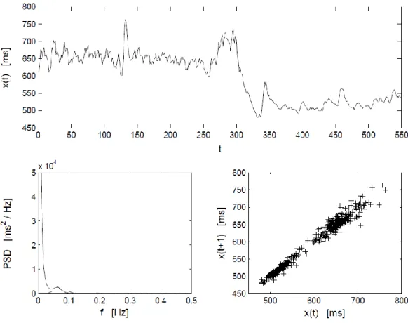
Figure 16. RR time series ... 58

Figure 17. Wavelet signal decomposition presented by a tree structure ... 74

Figure 18. Sub band filtering procedure using filter banks ... 75

Figure 19. Wavelet packet signal decomposition ... 76

Figure 20. Typical ECG signal with noise... 77

Figure 21. Various coefficients for an ECG signal ... 80

Figure 22. Example of noise free ECG ... 81

Figure 23. Matrix ... 82

Figure 24. Comparison of filtered ECG and noise free ECG ... 84

Figure 25. Fluctuation function vs. time lag plotting ... 87

Figure 26. Hi-Low variability periods ... 89

Figure 27. Multi-scaling behavior ... 91

Figure 28. PVC graph ... 94

Figure 29. Bigeminy graph ... 94

Figure 30. Couplet graph ... 95

Figure 31. Atrial Flutter ... 96

Figure 32. Atrial Fibrillation ... 96

Figure 33. Ventricular Flutter ... 97

Figure 34. Ventricular Flutter (continued)... 97

Figure 35. T-wave alternans taken from ECG tape ... 103

Figure 36. Imitation of TDP in ECG signal ... 105

Figure 37. Repolarization map ... 108

Figure 38. Heart beat ... 109

Figure 39. The circuit ... 111

Figure 40. The PCB ... 112

Figure 41. The populated prototype board explained ... 113

Figure 42. Output of NSR ... 116

Figure 43. SNR in 10 secs ... 116

Figure 44. Programs starting page ... 117

Figure 45. Figure 43 with 47 ... 117

Figure 46. The program ... 120

Figure 47. Spline Fit ... 122

Figure 48. Spline fit in program ... 125

Figure 49. pp.coef of the spline fit... 126

Figure 50. Standard deviation of 4 coefs. ... 127

Figure 51. Patients performing ECG ... 128

Figure 52. Child performing ECG ... 129

Figure 53. The main tools for data collection, measurement and process ... 131

Figure 54. Simulaids interactive ECG simulator ... 132

Figure 55. NSR ... 133

Figure 56. VTFast ... 134

Figure 57. VTslow ... 134

Antonopoulos John – PHD Research Page 9

Figure 62. ASYS ... 137

Figure 63. Data with necessary groups ... 140

Figure 64. 3D graph of factors 2, 3 and 4 ... 141

Figure 65. Linear fit ... 141

Figure 66. Figure 64 including the actual heart signals ... 142

Figure 67. Figure 67 with the necessary grouping ... 143

Figure 68. VF simulated signals with the actual VF patients ... 143

Figure 69. VT poly simulated signals with the actual VT poly patient ... 144

Figure 70. SVT simulated signals with the actual SVT patients ... 144

Figure 71. AFIB simulated signals with the actual AFIB patients ... 145

Figure 72. NSR simulated signals with the actual healthy people ... 145

Figure 73. The group of 4 actual healthy people ... 146

Figure 74. A ―normal‖ ECG VS a ―stressed‖ ECG of the same individual person ... 147

List of Tables: Table 1. Model of a normal ECG ... 31

Table 2. Results obtained from the baseline simulation done on 650 artificial test signals .... 83

Table 3. Heart p-values of the test ... 92

Table 4. Comparison between measured BPM and actual BPM based in bibliography ... 138

Antonopoulos John – PHD Research Page 10 AIC - Akaike information criterion

AGC - Automatic gain control AMI - Acute myocardial infarction ANS - Autonomic nervous system AP - Action potential

APD - Action potential duration AR – Autoregressive

AV – Atrioventricular

BSP – Body Surface Potentials CHF - Congestive heart failure CO - Cardiac output

CSA - Compressed spectral arrays CTM - Measure of central tendency CWT - Continuous wavelet transform CV - Coefficient of variation

DWD - Discrete Wigner distribution DWT - Discrete wavelet transform ECG - Electrocardiogram

FIR - Finite impulse response FFT - Fast Fourier Transform FHRV - Fetal heart rate variability FPE - Final prediction error HF - High frequency HR - Heart rate

HRV - Heart rate variability LF - Low frequency

LF/HF - The ratio of the power estimates for the LF and HF components LMS - Least mean square

MAP - Monophasic action potential MI - Myocardial infraction MP - Matching pursuit

NN sequence - Normal Sinus to Normal Sinus sequence PCA – Principal Component Analysis

pNN50 - The percentage of difference between adjacent normal RR intervals greater than 50 ms computed over the entire 24 hour ECG recording

QMF - Quadrature mirror filter

QRS - Q-, R-, and S-waves in electrocardiogram QT - QT time interval

Antonopoulos John – PHD Research Page 11 RT - RT time interval

RWED - Running windowed exponential distribution SA - Sinoatrial

SD - Standard deviation

SDA - Selective discrete Fourier transform algorithm

SDANN - Standard Deviation of the Averages of NN Intervals in All 5-Minute Segments of a 24-Hour Recording SDNNIDX - The mean of the standard deviations of all normal RR intervals for all five minutes segments of a 24 hour ECG recording

SVM – support vector machines

SPWD - Smoothed pseudo Wigner distribution STFT - Short-time Fourier transform

SV - Stroke volume

SURE - Stein's unbiased risk estimate TFR - Time frequency representation

TI NN - Triangular interpolation of the normal-to-normal histogram ULF - Ultra low frequency

VLF - Very low frequency

VRD - Ventricular repolarization duration WD - Wigner distribution

WP - Wavelet packet WT - Wavelet transform

Antonopoulos John – PHD Research Page 12

1. Introduction

1.1 Aims of investigation

In 1992, 42% of adult deaths in USA was caused by heart diseases as scientific researches point that as the mean average of population getting older heart diseases are growing. A timely diagnosis and prevention is very needful and also there is a tension to avoid costly and same times dangerous methods of examination and surgical operation.

Electrocardiogram is common practice for diagnosis of heart diseases and is based on measurement of electrical activity on the body surface caused by the function of heart.

Eithoven in 1903 developed further the theory of cardiac signals which was acquaintance from 1889, while he is also the person in charge for the import of significances that is used until today while it determined and the points from which the signals should be received. Finally it developed the basic theory round the ECG, central regard of which is the modelling of heart as a time-rating dipole.

The fundamental practice for recording the cardiac signals is the measurement of a voltage difference between two points in the body. Eithoven had assign three leads (I, II, III) derived from the arms and the left leg. Since then, 9 other leads developed in order the examiner to have a complete picture of the heart function.

The Einthoven three lead recordings are reported with Latin numbers I, II, III. These are defined as:

I = B LA – B RA

II = B LL – B RA

III = B LL – B LA

where RA = Right Arm, LA = Left Arm, LL = Left Leg. The three signal recordings are not independent of each other but are related with II = I + III.

In today it is scientifically accepted that the same diseases in two different patients have the same influence in the cardiosignal and differentiate its morphology

Antonopoulos John – PHD Research Page 13 in the same way giving us the opportunity to recognize the disease. The unchangeable morphology of the two derivatives of the cardiosignal gives also the possibility to proceed in the study and creation of patterns that recognize the disease. So, patients that are examined have the same heart disorders in order to see which parameters of the cardiosignal remain stable, which change and if there is any relation between this change and the gravity of the disease. Another way to exam the heart functionality is by measuring the chaotic morphology of the cardiac signal.

The principal aim of the project is to develop new algorithms for analysis of the electro cardio signal waveform and also to create a portable and accurate ECG analyser in order to succeed a) timely diagnosis, b) avoid costly diagnosis, c) improvement of today methods, d) improve the pro- surgical planning –decrease the surgical risk and e) supply the research of the heart and heart diseases.

In order to success the original goal, initially a development of an ECG analyser containing new and powerful signal processors and also analog filters had to be made. A computer software developed in Matlab for analysing the cardiac signals, placing the input signals into digital filters and lead to scientific results about the methodology and the diagnosis of a disease followed and initiated the research.

1.2 Project Objectives

The principal objectives of the work are:

 Literature survey of previous and current developments in the field.

 Develop (design and construction) of an electro cardiographer with high resolution in very low bio-electrical signals. Portable and connectable with computers.

 Development of software in Matlab based on the theoretical analysis about these bio-signals. This program will provides the possibility of a very circumstantial analysis of cardiac signals either to time domain or to frequency domain.

 Creation of a database consisted of simulated cardio signals categorized in groups. A deep mathematical, physical and statistical analysis will be carried out in order to find any common points between signals of the same disease or

Antonopoulos John – PHD Research Page 14 even a pattern than a disease follows and change the cardiac signal in the time domain, frequency domain, first and second derivative or chaos.

 Further development of the software in order to be able to compare new signals with signals of the database and through an analysis of derivatives, chaos and a comparison is capable for diagnosis.

 Compare real human samples with the theoretical model.

 Finalization of the portable device and statistical analysis of the capability.

1.3 Summary

In the following chapter of the research, a detailed analysis of the way a human heart works and sends biosignals throughout the body is explained. A more comprehensive analysis of the cardiovascular signals is quoted.

In chapter three, a physiological background of the heart is analyzed thoroughly with the analysis of signal variability to be expanded in every detail. Notable interest shows the induction of chaos theory in ECG in this chapter. Another very interesting part of this chapter is where common heart rhythms and arrhythmias are explained.

In chapter four the methods of investigation are discussed. This includes not only the ECG hardware created for this research, but also the software that was implemented with the application "MATLAB". The ways of acquiring an ECG from adults and kids are also mentioned.

The main function used in this research, that is Cubic Splines, and the necessary routine creation are thoroughly explained in chapter five. Here the main simulating device used for exporting various heart conditions in order to create a well established signal database is introduced. A way to correlate the factors of the various heart conditions collected and analyzed is explained and presented with real human samples compared with the theoretical model.

In the last chapter, conclusion and further development of the research are presented.

Antonopoulos John – PHD Research Page 15

2. Literature survey

2.1 The heart and electrical signals

The human heart, one of the most studied organs in biology, is a hollow mass of mainly striated muscle fibers. It is situated slightly to the left of the middle of the thorax, underneath the breastbone (the sternum), at a position surrounded by the lungs (Figure 1). It is most essential to life, since its function is to pump blood through the blood vessels to the entire body by repeated, rhythmic contractions. It is the active center of the human cardiovascular system, circulating blood in the entire organism as a medium for transporting substances such as oxygen, nutrients, blood cells, enzymes, antibodies, as well as collecting the corresponding counterparts as wastes, toxins or external agents for disposal.

Figure 1. Heart and lungs.[1]

The heart consists of four chambers, namely the two upper atria and the two lower ventricles. The number of chambers followed the evolutionary pattern of the

Antonopoulos John – PHD Research Page 16 vertebrates, which prevents a blend of arterial and venous blood in the closed circulatory system.

The high energy consumption of homeotherms, i.e. the avian and mammals, requested a higher efficiency of oxygen transport by clearly separating oxygenated and deoxygenated hemoglobin within the circuit. Indeed, the number of the chambers in the heart in terms of their specific functions as well as their structures and geometries are important in the expression of the pathology of this organ studied in this work. The atria serve as buffers for blood entering the heart from which it is transferred to the ventricles. The ventricles are the actual pumps that propel the blood into the circulatory system. The valves between the atria and ventricles maintain coordinated unidirectional blood flow from the atria to the ventricles. Thevenous blood returning from the peripheral vessels enters the right atrium, through which it passes to the right ventricle and is sent to the lungs through the pulmonary artery. The blood, rich with oxygen and free of carbon dioxide by diffusion at the pulmonary alveoli, is passed to the left atrium from which it enters the left ventricle. The latter forces the blood into the aorta from which it enters the entire circulatory system (figure 2).

Figure 2. Heart as the main pump of the cardiovascular system. Schematic diagram of blood flow in the human heart and nomenclature of principal anatomical

Antonopoulos John – PHD Research Page 17 Every normal single beat of the heart involves a sequence of these well-organized events, which constitutes the cardiac cycle. In a cardiac cycle, the aforementioned sequence consists of three major stages, namely the atrial systole, the ventricular systole and the complete cardiac diastole. The atrial systole is the phase which comprises the contraction of the atria and the corresponding influx of blood into the ventricles. Once the blood has fully left the atria, the atrioventricular valves close, preventing backflow into the atria. This closing of the valves (semilunar and atrioventricular) is the origin of the familiar beating sounds of the heart. The ventricular systole consists of the ventricular contraction and the efflux of blood into the circulatory system. Once the blood is expelled from the ventricles, the pulmonary and aortic semilunar valves close. The final complete cardiac diastole involves the relaxation of the atria and ventricles in preparation for the refilling phase of circulating blood. The whole cycle of blood circulation within the system is governed almost completely by the fluid mechanics regulated by the muscular contraction of the heart.

2.1.1 Bioelectricity of the heart

The cardiac muscle, a spontaneously contracting, self-exciting tissue, develops the driving force governing the fluid mechanics of the circulatory system by converting biochemical energy to kinetic energy. The contraction of the muscle is triggered by an electric stimulation, that is, the onset of a bioelectric signal called the action potential (AP).

Antonopoulos John – PHD Research Page 18 The action potential is the general term for an all-or-none active electric impulse traveling along the cell membrane (Figure 3).

In the neural system, it functions as a messenger between cells, while in muscles, it regulates the contraction of fibers. It is generated by exchanges of electrically charged ions across the cell membrane via ion channels, [3] creating a local potential bias above a triggering threshold between the two sides of the membrane. In its relaxed state, the inside of a cardiac myocyte is at a negative potential with respect to the outside, the resting potential. If the absolute value of this resting potential is reduced below a threshold level, a cascade of ion kinetics is induced, entailing chain reactions of potential dynamics propagation to the surrounding cell membrane (figure 4).

The resting potential of a cell membrane is generated by an electrochemical equilibrium of charges (ions) on each side of the membrane. The action potential reflects the local acute non-linear depolarization from this resting potential, followed by a repolarization phase of return to the resting potential.

Antonopoulos John – PHD Research Page 19 The dynamics of the inward and outward electric current is regulated by the opening and closing of the gates (ion channels) and is ruled by the electrochemical diffusion of the ions [5]. The transport of ions that regenerate the initial equilibrium is an active procedure carried out by the ion pumps. There is a brief time interval, called the refractory period, during which the membrane is not excitable between two successive action potentials.

In the case of cardiac muscle, the action potential is the signal that activates the contraction of the cardiomyocytes by propagating from cell to cell over the whole tissue. There are, nonetheless, preferential pathways along fast conducting bundles that effect the organization of the contraction of the chambers.

Figure 5. Temporal relationships between the ventricular action potential (top) and the ECG (bottom). The QRS complex, T wave and QT interval are indicated. Both signals are functions of the same timescale on the x axis; the y axis plots voltage, with a gain that is roughly 100-fold higher for the ECG than for the action potential (that

is, the absolute signal amplitude is about 100-fold smaller for the ECG).[6]

The rhythmic sequence of the cardiac cycle is initiated by the sinoatrial (SA) node and regulated by the atrioventricular (AV) node. The sinoatrial node, known as the cardiac pacemaker, is located in the upper front wall of the right atrium and is responsible for the initiation of action potential propagation that contracts the atria. Once the propagation reaches the atrioventricular node, situated in the lower right atrium, it is conducted through the bundle of His, the left and right bundle branches, and to an extensive network of Purkinje fibers which trigger the contraction of the

Antonopoulos John – PHD Research Page 20 ventricles. The AV node regulates the timing of transmission of the excitation to the ventricles, creating a delay between the contractions of the two groups of chambers which enhances the filling of the ventricles prior to their contraction.

The physiological activity of the myocardium involves associated electromagnetic phenomena that are expressed as electric potential dynamics inside the entire body. As early as in the 19th century it became clear that the heart generated electricity. The first to systematically approach the heart from an electrical point of view was Augustus Waller, working in St Mary‘s Hospital in Paddington, London. [7] He used a mercury capillary electrometer to measure the electromotive changes on the body surface arising from the beat of the mammalian heart, and of the human heart in particular (figure 6).

Antonopoulos John – PHD Research Page 21

2.1.2 Body surface potentials and Electrocardiogram

The electromagnetism linked to the electrophysiology of the heart is a direct expression of the cardiac mechanical function. Hence, the observation of the electric activity as body surface potentials (BSP) is an efficient and non-invasive manner of estimating the functional state of the heart. The time course of the resulting potential differences between any two points on the body surface is called Electrocardiogram (ECG).

Figure 7. Picture of an early ECG recording performed by Willem Einthoven in 1903.[8]

Following Waller, a major breakthrough in cardiac electrophysiology was reached when Willem Einthoven, working in Leiden, the Netherlands, used a string galvanometer in 1901 to record ECGs. By measuring the potential differences between the two hands and the left foot (figure 7), Einthoven assigned the letters P, Q, R, S and T to the various deflections, and described the electrocardiographic features of a number of cardiovascular disorders.[9] He received the Nobel Prize in Physiology

or Medicine for his discovery in 1924.

Nowadays, the electrodes used in clinical practice to record the standard

Antonopoulos John – PHD Research Page 22 precordial positions (V1 to V6) as presented in figure 7. These nine electrodes located over the surface of the human body capture the electric activity of the heart from different angles reconstructing the spatial dynamics of the heart‘s electric activity. A display of the three limb leads in the form of a triangle on the frontal plane is referred to as Einthoven‘s triangle. The mean value of the instantaneous potentials is used as the reference of the ECG signals, known as the Wilson Central Terminal (WCT) reference (figure 8). The ECG is the prime tool in cardiology, and has its main function in screening and diagnosis of cardiovascular diseases in clinical practice. Because of the strong link (direct and indirect) between cardiac function and electric potential dynamics observable on the body surface, many cardiac diseases can be monitored through the expressed potential differences.

Figure 8. Electrode positions of a standard 12-lead ECG and the derived leads. The three limb electrodes form an equilateral triangle in the frontal plane called the

Einthoven triangle (right panel). The potential reference for all other leads is Wilson‟s Central Terminal (WCT) defined as the mean value of the potentials at electrodes VR, VL and VF, corresponding to the position of the center of gravity of

Einthoven‟s triangle.[4]

According to the well-established definition of waveforms observable on each lead, the ECG has a wide use for indicating pathologies such as cardiac arrhythmias, ischemia, or conduction abnormalities.

Antonopoulos John – PHD Research Page 23 Figure 9. An example of standard ECG recording during normal sinus rhythm. The twelve derivations are potential differences specifically defined between electrodes. I, II and III are potential differences between the limb electrodes as shown

in figure 8. aVR, aVL and aVF are the “augmented” VR, VL and VF, respectively, signifying the 1.5-fold voltage between the corresponding electrode and the WCT reference. This is a historical custom in which, for instance, aVR was measured as VR

– (V L + V F), which simply resulted as aV R = VR. V1 to V6 are the potential

differences between the corresponding precordial electrodes and the WCT reference.[4]

2.1.3. Electrophysiology

Electrophysiology is the study of the electrical properties of biological cells and tissues. It involves measurements of voltage change or electric current on a wide variety of scales from single ion channel proteins to whole organs like the heart. In neuroscience, it includes measurements of the electrical activity of neurons, and particularly action potential activity. Classical electrophysiology techniques involve placing electrodes into various preparations of biological tissue. The principal types of electrodes are simple solid conductors, such as discs and needles (singles or arrays), tracings on printed circuit boards, and hollow tubes filled with an electrolyte, such as glass pipettes. The principal preparations include first of all living organisms, excised tissue (acute or cultured), dissociated cells from excised tissue (acute or cultured), artificially grown cells or tissues, or hybrids of the above. [10]

Many particular electrophysiological readings have specific names: For the heart it is called Electrocardiography

Antonopoulos John – PHD Research Page 24 For the brain Electroencephalography

From the cerebral cortex Electrocorticography For the muscles Electromyography

For the eyes Electrooculography For the retina Electroretinography

For the olfactory receptors in arthropods Electroantennography For the auditory system Audiology

2.1.3.1. Electrophysiology of the Heart

Like all living cells at rest, the cardiac muscle cell or myocyte is polarized, so that the potential inside the cell, which called intracellular space, is negative with respect to the outside, which called interstitial space.

The transmembrane potential is defined as the potential difference across the surface membrane of the cell. It is controlled primarily by three factors. The first is the concentration of ions on the inside and outside of the cell, particularly , , , and . The second factor is the permeability of the cell membrane to those ions through specific ion channels. The last factor is the activity of electrogenic pumps (e.g., / -ATPase and Ca2+ transport pumps) that maintain the ion concentrations across the cell membrane. Because K+ concentration is high inside the cell and low outside, a chemical gradient for K+ to diffuse out of the cell is found. In opposite, and chemical gradients for an inward diffusion are found. The natural tendency of sodium and potassium ions is to diffuse across their chemical gradients to attempt to reach their respective equilibrium potentials, with sodium diffusing into the cell and potassium diffusing out.

However, the resting cell membrane is approximately 100 times more permeable to potassium than to sodium, so that more potassium diffuses out of the cell than sodium diffuses in. This permeability to potassium is due to potassium channels that are open at the resting voltage. As a result, the dominant outward leak of potassium ions produces a polarizing current that establishes the cell‘s resting potential of roughly -70 mV [11].

Antonopoulos John – PHD Research Page 25

2.1.3.2. The Action Potential of a Single Cell of Working

Myocardium

By applying an external stimulus, cells of excitable tissues can be polarized. An action potential can be produced by a sequence of influx and out flux of multiple captions and anions through the cell membrane. Once a cardiac cell is getting excited, an electrical stimulation to the cells that lie adjacent to it and furthermore to all the cells of the heart will be propagated [12]. The action potential has five phases, numbered from zero to four. A typical action potential for a cardiac myocyte in the left ventricle is shown in figure 10.

Figure 10. The Action Potential of a single cell of working Myocardium.[13]

Phase 4 represents the resting transmembrane potential, in other words, this voltage can be measured if the cell is not stimulated. This phase of the action potential is associated with the diastole of heart chambers. Phase 0 is known as the rapid depolarization phase. The maximum rate of depolarization of the cell, /dt, is determined by the slop of curve corresponding to this phase. This phase is associated with opening of the fast channels, rapidly increasing the membrane conductance to (gNa) and a rapid influx of ionic current (INa) into the cell. In fact, the

Antonopoulos John – PHD Research Page 26 fast sodium channel has two gates, the h gate and m gate, whose interaction allows to enter the cell through this channel. At rest, the m gate is closed and h gate is open, but when the transmembrane potential approaches a threshold (about -60 mV), the m gate opens quickly while the h gate closes slowly. After a very short time, both gates will be open changing the sign of the transmembrane voltage to positive value (round +20 mV), to the so-called overshoot. The closure of the fast channel after a short time and the slower outflow of potassium through the potassium channels are tending to restore the initial state of the membrane generating the phase 1. The balance between inward movement of (ICa) through Ltype calcium channels and outward movement of K+ through potassium channels sustains the phase 2 (or so-called plateau) of the action potential. Cardiac myocytes have different characteristics of the plateau phase. During this phase the fast sodium channels are not active keeping the cell immune to any external stimulus. Therefore, it is called refractory period. In the phase 3 of the action potential, will be accumulated in the xtracellular space leaving the intracellular space. This action is responsible for the repolarization of the cell. The cell can be depolarized again in this period by very large stimuli, therefore it is called refractory relative period. Finally, channels close when the transmembrane potential is set back to the resting phase and the initial concentration of ions is rapidly restored by means of Na-K pumps and Na-Ca exchangers. The myocytes throughout the heart have different time course of action potentials (figure 11).

Antonopoulos John – PHD Research Page 27 Figure 11. The resting voltage and action potential electrophysiology of a single cell

of working Myocardium[14].

2.1.3.3. Excitation Propagation and Cardiac Contractions

Cardiomyocytes consist of three systems: a sarcolemmal excitation system that participates in spread of action potential (AP) and functions as a switch initiating intracellular events giving rise to contraction, an intracellular excitation-contraction coupling (ECC) that converts the electric excitation signal to a chemical signal and activates the contractile system, a molecular motor based on formation of chemical bridges between actin and myosin.

1. The Excitation System: This system is responsible to maintain the resting potential, create an action potential and facilitate spreading the AP. The cardiac cycle

Antonopoulos John – PHD Research Page 28 is initiated from the excitation system of SA node. The rapid change in the voltage during an AP causes the activation in the excitation system. Consequently, the neighboring cells will be depolarized. As a result, an electrical impulse, also called the cardiac electrical wavefront, propagates through the conduction system of the heart and spreads from cell to cell throughout the myocardium in the way that the atrial and ventricular contraction (depolarization) and relaxation (repolarization) will happen with the correct timing in the healthy heart [15].

Figure 12. Schematic diagram of the major cellular components involved in contraction of the myocyte.[16]

2. The Excitation-Contraction Coupling System: Excitation-contraction coupling (ECC) is established by the sarcotubular system, an arrangement of specialized sarcoleman and intracellular membranes that controls and amplifies the ability of AP to switch the contractile system on and off by creating electrochemical signals between the sarcolernma and intracellular organelles. When a myocyte is

Antonopoulos John – PHD Research Page 29 potential through L-type calcium channels triggering a subsequent release of calcium that is stored in the sarcoplasmic reticulum (SR) increasing the

intracellular calcium concentration from about 10-7 to 10-5 M. The released

calcium binds to troponin-C (TN-C) that is part of the regulatory complex attached to the thin filaments. When calcium binds to the TN-C, this induces a conformational change in the regulatory complex such that troponin-I (TN-I) exposes a site on the actin molecule that is able to bind to the myosin ATPase located on the myosin head. This binding results in ATP hydrolysis that supplies energy fora conformational change to occur in the actin-myosin complex [17].

3. The Contractile System: The building block of the contractile system is the sarcomere. The result of the changes made by the released calcium in ECC is a movement between the myosin heads and the actin. The actin and myosin filaments slide past each other thereby shortening the sarcomere length. This ratcheting cycle occurs as long as the cytosolic calcium remains elevated. At the end of phase 2 of APcycle ends when new ATP binds to the myosin head, displacing the ADP and the initial sarcomere length is restored.

2.1.3.4. The Generation of an Electrocardiogram and the

Dominant Cardiac Vector

The Electrocardiogram (ECG) represents a temporal and spatial summation of the extracellular fields of the action potentials generated by millions of cardiac cell. It describes the different electrical phases of the cardiac cycle. ECG provides a measure of the electrical currents generated in the extracellular fluid by the changes in the APs. At any given instant, only a group of cells out of millions of individual cells in the myocardium depolarizes simultaneously. They can be represented as an equivalent current dipole source to which a vector is associated, describing the dipole‘s time-varying position, orientation, and magnitude [15]. The dominant vector describing the main direction of the electrical wavefront can be defined as a summation of the vectors of all current dipoles in the heart at a certain time instant.

Antonopoulos John – PHD Research Page 30

2.2. Cardiovascular variability signals

The sinus rhythm fluctuates around the mean heart rate, which is due to continuous alteration in the autonomic neural regulation, i.e. sympathetic-parasympathetic balance. Periodic fluctuations found in heart rate originate from regulation related to respiration, blood pressure (baroreflex) and thermoregulation.

Parasympathetic (vagal) regulation to the heart is inhibited simultaneously with inspiration, and the breathing frequency coincides with fluctuations observed in heart rate [18]. Furthermore, thoracic stretch receptors and peripheral hemodynamic reflexes also result in respiratory arrhythmia [19]. Respiratory arrhythmias are consequently due to parasympathetic regulation and can be excluded by atropine or vagotomy [19]. The maximal amplitude of respiratory related heart rate fluctuation is found at breathing rate of 6 cycles per minute, because the fluctuation increases as respiration rate achieves the frequency of the intrinsic baroreflex-related heart rate fluctuations [20].

The fluctuations due to blood pressure regulating mechanisms originate from self-oscillation in the vasomotor part of the baroreflex loop [20]. These fluctuations coincide with synchronous oscillations in blood pressure called Meyer waves [21]. Increase of sympathetic nerve impulses strengthen and sympathetic or parasymphatetic blockade weaken these fluctuations in heart rate [22, 23].

Changes in peripheral resistance produce low frequency oscillations in heart rate and, for example, in systolic blood pressure. Thermal stimulation given on the skin can be used to stimulate the oscillations, which are originally due to thermoregulatory adjustment of peripheral blood flow [20]. These fluctuations are controlled by the sympathetic part of the autonomic nervous system.

The overall autonomic function is controlled by a central command from the brain. However, the autonomic nervous system operates as a feedback system, and heart rate is thus regulated by many reflexes which may increase or decrease the sympathetic or parasympathetic activity or both of them [24]. Reflexes can act simultaneously and their interactions may be complex. The arterial baroreceptor reflex originates from receptors located in the arteries such as carotid sinuses and aortic arch. The increase in blood pressure excites baroreceptors producing an

Antonopoulos John – PHD Research Page 31 augmented efferent vagal and reduced sympathetic activity. Peripheral arterial chemoreceptors located in the carotid and aortic bodies produce, most often, an increase in the rate and depth of respiration. Because this reflex influence on heart rate through respiration, the effects may be covered by other respiratory responses. The coronary chemoreflex (Bezold-Jarisch reflex) can cause bradycardia and is significant in pathological states such as myocardial ischemia and infarction. Atrial receptors stretched by the increase in atrial volume and some of them by atrial contraction, the response being linked directly to atrial pressure. These volume receptors cause an increase in heart rate and operate through the sympathetic nerves producing their response very slowly. There exist also other cardiovascular reflexes coming from receptors located e.g. in pulmonary arteries, lungs and muscles.

The physiological importance of heart rate can be demonstrated by an axiomatic relation in which cardiac output (CO) can be defined by a product between heart rate and stroke volume (SV) as CO = HR ·SV. Because heart rate and stroke volume are not independent of each other, the definition of cardiac output is not always so straightforward in terms of physiological adjustment.

The rate of depolarization of the cardiac pacemaker defines heart rate. The sinoatrial (SA) node, the atrioventricular (AV) node and the Purkinje tissue can be regarded as potential pacemaker tissues in a heart. As the fastest depolarization rate is found in the sinoatrial node and the depolarization impulse spreads through the conduction system to other pacemakers before they spontaneously depolarize, the sinoatrial node usually defines the heart rate. However, failing to produce a normal pacemaker impulse, other pacemaker tissues can act as a cardiac pacemaker.

Antonopoulos John – PHD Research Page 32 Figure 13. ECG Analysis

Autonomic neural regulation of the heart is determined by its sympathetic and parasympathetic parts. The parasympathetic nerves are connected to the sinoatrial node, the AV conducting pathways and the atrial and ventricular muscles as well as coronary vessels. Sympathetic nerve fibers innervate the SA node, the AV conducting pathways, coronary vessels and the atrial and ventricular myocardium [25]. Both divisions of the autonomic nervous system always have some activity which continuously regulates the function of the heart. Heart rate response therefore presents a balance between sympathetic and parasympathetic (vagal) regulation which can be considered also as an antagonist function.

Heart rate has a major effect on ventricular repolarization duration (VRD), but the autonomic nervous system also regulates directly the repolarization of the ventricles. In addition, electrolytic factors, age and gender have an effect on it. It has been shown that when the autonomic nervous system regulates VRD there are similar periodic fluctuations as seen in heart rate [26].

2.2.1. Changes of signal variability connected to

specific diseases

A decrease in vagal neural activity into the heart may result in diminished HRV after myocardial infarct (MI) leading to the prevalence of symphatetic neural

Antonopoulos John – PHD Research Page 33 regulation and to electrical instability [27]. Reduced heart rate variability is also associated with an increased risk for ventricular fibrillation and sudden cardiac death [28, 29]. Changes in long term RR interval dynamics with beat-to-beat RR interval alternans is concluded to precede the spontaneuous onset of sustained ventricular tachyarrhythmias [30]. Results obtained using spectral analysis of HRV suggests a change of sympatho-vagal balance toward symphatetic dominance and a diminished vagal tone in patients surviving an acute myocardial infarction [27, 31]. Cardiac diseases such as congestive heart failure, coronary artery disease and essential hypertension are also associated with a reduced vagal and an enhanced sympathetic tone, which change heart rate variability dynamics [20, 32]. Because HRV analysis can be regarded as a noninvasive, reproducible and an easy to use method reflecting the degree of autonomic control of the heart [33], it has been widely used to diagnose the autonomic dysfunction due to diabetic neuropathy (34, 35, 36]. It has been generally observed, that overall HRV is reduced and sympatho-vagal balance may be altered during tilt maneuver or standing in diabetic patients [32, 25].

Although HRV is used in a wide range of clinical applications, diminished HRV has only been generally accepted as a predictor of risk after acute myocardial infarction and as an early warning of diabetic neuropathy. Diminished HRV can predict mortality and arrhythmic events independently of other risk factors after acute myocardial infarction, and long-term HRV analysis have proven to be a more definite predictor compared to a short-term analysis [27]. Heart rate variability analysis should also be joined with other risk factors so as to improve the predictive use. Any heart disease (left ventricular hyperthrophy, heart failure, etc.) can modify repolarization duration [37]. Anomalies in repolarization duration are signs of electrical instability in the heart and can lead to malignant arrhythmias such as ventricular fibrillation and Torsades de Pointes. Analysis of ventricular repolarization duration dynamics provides essential information on a propensity for ventricular arrhythmias, because some life-threatening arrhythmias arise in myocardial tissue. Altered dynamics of the VRD, and the events of the alternating T wave amplitude particularly in patients with the long QT syndrome as well as with structural heart disease at fast heart rates, suggest that the analysis of the ventricular repolarization dynamics may provide an important clinical tool [38].

Antonopoulos John – PHD Research Page 34

2.2.2. Other events modifying signal variability

Several pharmaceutical interventions can be used to modify heart rate dynamics as shown by human [39] and animal [3] studies. Atropine administration has been used to prove the connection between vagal neural activity and high frequency (respiratory related) fluctuation in RR interval time series [23]. Scopolamine significantly augments heart rate variability [40] which suggests an increasing coincident vagal activity into the heart. The effect of β-adrenergic receptor blockades has been studied after myocardial infarction [41, 42]. There are also studies on the effect of antiarrhythmic drugs such as flecainide and propafenone, as well as encainide and moricizine on the heart rate dynamics [31, 43, 5]. A study of the effect of β-adrenergic blocker (nadolol) on ventricular repolarization duration and its dynamics was made. The finding was that the length of repolarization duration was shorter, the signal variance was greater and the spectral pattern was shifted to higher frequencies due to this medication. A change of the dynamic relationship between ventricular repolarization duration and heart rate has been observed as a consequence of nadolol administration with normal patients [26, 44].

Heart rate variability has been employed to investigate the short and long term autonomic responses to physical and mental exercise. It has been observed that the increase in respiratory related fluctuation, the total HRV reduction and the recorded signal become more nonstationary as the intensity of the dynamic physical exercise increases [45]. Heavy physical exercise has been shown to augment low-frequency (LF) fluctuations in heart rate, and the recovery of the spectral pattern may last even 48 hours after finishing exercise [46]. The sympatho-vagal balance seems to change towards sympathetic dominance e.g. in hypertensive patients. Long term physical exercise has positive effects on hemodynamics and neural control mechanisms, for example, by lowering the arterial pressure in hypertensive patients [47] and increasing baroreflex gain in patients with ischemic heart disease [48] An overall observation, also related to dynamic mental stress, is an increase of the sympathetically- and a decrease of vagally-mediated fluctuations in heart rate [7].

Antonopoulos John – PHD Research Page 35

2.2.3. Various time series

RR interval time series

The basic procedure used for determining the heart rate and its fluctuations is described below. An electrocardiogram (ECG) is measured, using appropriate data acquisition equipment. The time elapsing between consecutive heart beats is defined as that between two P waves, when a P wave describes the phase of atrial depolarization. In practice, it is the QRS complex that is used to obtain the time period between heart beats. This complex is detected in the R wave, because it has a very clear amplitude and better frequency resolution than the P wave, and a much better signal-to-noise ratio. The time interval between the P and R waves can be assumed and has been shown to be constant [21]. Defining the times of occurrence of two consecutive R waves as s(t) and s(t+1), t = 1,…, N, the expression

is obtained for a time period in milliseconds. This x(t) is called the RR interval time series or else the times to which it refers are simply called RR intervals. A heart rate time series [min−1] can be obtained by y(t) = 1000 · (60/x(t)) and the mean heart rate is simply . These formulae indicate a nonlinear relationship between the values in a given time series, which should be taken into account when comparing the results obtained by time and frequency domain approaches [49]. At the moment, RR intervals seem to be the more frequently used time series in heart rate variability (HRV) analysis. For a discussion of the choice between different time series (tachograms), [50]

VRD time series

QT time interval in electrocardiographic signals has been used to perform both static and dynamic analyses of the duration of the ventricular repolarization. There exist difficulties in the detection of the onset of Q wave and the offset of T wave due to poor signal-to-noise ratio and varying ECG morphology. For these reasons other

Antonopoulos John – PHD Research Page 36 estimates, such as RTmax interval, has been widely used. Moreover, this provided a motivation to investigate and compare the noise sensitivity of different

QT interval estimates. Because Q-S time interval is a result of the depolarization period of the ventricles, it is actually more correct to measure the time interval between the R and T waves as one is interested in the changes occurring within the ventricular repolarization period. R wave has been used to estimate the start of the repolarization period because searching for the offset of S wave can be difficult. The maximum (apex) of T wave has been often regarded as a more reliable estimate for the end of the repolarization period than the T wave offset. The total repolarization duration, i.e. time interval between the offsets of S and T waves, can further be analyzed with respect to early and late repolarization duration as well as repolarization area [51]. In this work the objective will be on the measurement of the repolarization duration in the ambulatory ECG.

The 24-hour ambulatory ECG has certain problems and drawbacks because the signal is corrupted by noise from various sources and also several conditions may alter the ECG morphology. The ambulatory ECG is usually acquired with a sampling frequency of 128 Hz giving a time resolution of 7.81 ms for each sample, which is too low for QT interval variability measurement. It has been suggested that the QT interval should be determined at least with resolution of 1 ms, which would require 1 kHz sampling frequency for ECG signal. In an ambulatory measurement setting, with data acquisition times lasting up to 24 hours, the sampling frequency cannot be that high, because then the amount of the stored data rises rapidly. In present ambulatory ECG analysis systems the possibility of exporting a beat-to-beat QT time series extracted with high time resolution is also lacking. These problems have been solved by exporting raw ECG data and, by oversampling ECG signal [52] or by interpolating waveforms [53] a better time resolution for the time interval measurement results.

APD time series

The local ventricular repolarization duration can be measured by placing a contact electrode in a ventricular muscle. Rate-dependent dynamics of VRD obtained from the right ventricular apex provides an example. This approach can solve the above mentioned problems related to the ambulatory QT measurement. However, measuring monophasic action potentials (MAP) is an invasive procedure. The

Antonopoulos John – PHD Research Page 37 duration of repolarization phase, which is termed as action potential duration (APD), is estimated as a time interval between the onset and offset of the action potential. The offset is defined as the maximal positive derivative of the upstroke phase of the action potential waveform. The offset can be defined at time points where the waveform has come down 15, 30, 50 and 90 % from the maximal amplitude of the MAP. Most often used definitions are 50 and 90 % points. The APD time series are extracted from the consecutive waveforms and the beat-to-beat analysis is performed.

2.2.4. ECG waveform detection

The RR and QT interval measurement [54] was based on an implementation of an algorithm described previously [55] and the detection scheme will be briefly reviewed here. The basic concept of the algorithm is to look for the zero crossing points, the crossings of certain experimentally-determined threshold values, as well as the local maximum or minimum values of the differentiated ECG signal d(t) and its low-pass filtered version f(t).

The differentiator and the low-pass filter were modified according to the sampling rate in order to obtain an optimal frequency response. The sampling rate of the analyzed ECG was one parameter of the waveform detection procedure and in this way, the preprocessing filters and the algorithm itself can adapt to the different sampling rates.

The flowchart of the implemented waveform detection procedure is shown in Tikkanen‘s work [54] The first step is to calculate the signals d(t) and f(t), which is done for the whole period of the ECG selected for analysis. The waveform detection procedure continues by determining the initial value of the threshold value used to search the maximum absolute value of the QRS in the signal f(t). The threshold value

Hn+1 is continuously updated during the waveform detection using the equation [55].

,

(2.1)

Where is the absolute value of the signal f(t) at the detected fiducial R wave position of the beat n.

Antonopoulos John – PHD Research Page 38 The initialization of the average of RR intervals and the first RR interval value are then obtained. The value is later used to check the calculated value of a new RR interval and thus provides a basis for identifying the QRS complex.

The initial position of a QRS complex is detected using an adaptive threshold method determined by the RR interval average value [54]. After that, the algorithm continues to search the position of the R wave. In the present approach, the fiducial point of the R wave was detected using three methods: at the maximum amplitude upwards or downwards from the baseline, or at the zero crossing point of the signal

f(t) during the QRS complex. The last technique was implemented in the original algorithm by Laguna et al. (1990). It was found that, in some cases, a more accurate definition can be obtained, if the fiducial point of the R wave is defined at the maximal upward amplitude of QRS. With this algorithm, an accurate determination of the R wave is an absolutely necessary condition for a reliable Q wave detection. After detecting the R wave position and updating the threshold and , the onset of Q wave is searched keeping the R wave position as a reference point. Here it should be mentioned, that examining the pattern of the Q wave is made by analyzing the differentiated signal d(t) and not the signal f(t), because the signal d(t) includes the high frequency components of the Q wave. Next the T wave maximum and T wave end are detected from the signal f(t). The following definition for the limits of a search window calculated from the R wave position was used:

(2.2)

where a and b are parameter values in the procedure. This definition is a slightly different one from the given by Laguna et al. As the threshold for T wave end was used the value Hs = f(Ti)=2, Ti denoting the position of the maximal downward or upward slope after the T wave maximum.

Finally, a value of QT interval is calculated using the relation QT(n) = , where and are the positions of T wave end and the onset of the QT time interval during the beat n. The analysis of the next cardiac beat is started 150 ms after the last T wave end is defined.

The effects of the four alternative definitions of the QT interval onset on the analysis of QT interval dynamics were compared: true QRS onset, R wave maximum,

Antonopoulos John – PHD Research Page 39 ascending or descending maximal slopes of the R wave. One reason for this was quite practical: in some circumstances dealing with ambulatory ECG, the determination of the QRS onset seems to be uncertain e.g. because of a missing Q wave and the relatively low sampling rate. In the original implementation of this algorithm, the Q wave onset found is rejected if the difference between Q wave and R wave fiducially points are larger than 80 ms [55]. In that case, QRS onset is defined in the onset of R wave.

2.2.5. Ambulatory HRV data

The aim of recording RR intervals has been to gain information about the neural regulation of the heart and the circulatory system. Observing the changes occurring over long periods of time (i.e. several hours) requires ambulatory recording, which is usually performed using standard commercial equipment (Holter devices). This provides procedures for ECG signal acquisition and analysis, extracting the RR interval time series from the ECG signal and analyzing them. The sampling frequency typically used for an ECG signal with Holter devices is 128 Hz (as explained in 2.2.3.), which means a timing accuracy of 7.81 ms for R wave detection. Thus a low sampling frequency produces inaccuracies in RR interval measurement and bias in the analysis. A timing accuracy of the order of 1 ms would be desirable for the assessment of chaos, for example.

One factor affecting ambulatory HRV measurement is circumstances that vary with time, i.e. the fact that external conditions can be far from stable. This may produce nonstationary changes in a time series and make the assessment of the physiological events more difficult, or even impossible, than under stable laboratory conditions. A method for separating non-periodic (nonstationary) changes from periodic ones has been proposed by Sapoznikov D, Luria M & Gotsman M [59]. Variable conditions may also produce periodic fluctuations which become summed in the time series, making it difficult to distinguish the regulatory processes from each other. This can obviously lead to misinterpretations in some circumstances.

Antonopoulos John – PHD Research Page 40

2.2.5.1. Accuracy of HRV measurement

The accuracy of spectral estimates performed on RR intervals obtained from ambulatory Holter systems has been studied by Pinna G, Maestri R, Cesare AD, Colombo R & Minuco G [56]. It has been observed that the centre and dispersion of the estimation error changes from one Holter system to another. There are large inter-recorder differences and variable spectral distortion among selected spectral bands. Use of the Fourier spectral estimate gave more stable results than did the AR spectral estimate in ten minute ECG sequences. The main factor limiting the accuracy of the RR interval measurement was the low frequency with which the ECG signal was sampled, a topic discussed theoretically by various scientists [56, 57] concluded that spectral analysis of RR interval time series with very low variability may be seriously altered when performed on an ECG signal acquired using a Holter system.

The accuracy of spectral estimates of HRV was investigated by generating a simulated RR interval time series of variable length (180-540 seconds) using an autoregressive model from a set of recordings and adding Gaussian noise [58]. The accuracy of Fourier (Blackman-Tukey) and AR spectral estimates could then be evaluated in terms of the normalized bias and variance. The results showed that the bias (systematic error) of the estimate was a less important factor than the variance (random error). Both decreased as the length of the time series increased, but the variance decreased more rapidly. The power estimate was most stable in the HF band, while that in the VLF band had the highest variance. No minimum length was proposed for a time series, but it was concluded that even with the shortest record the bias made a less significant contribution to the estimates. It was pointed out that a relative high variability in spectral parameters is typical of RR interval time series, and that this should be noted in the analysis of the short time series.

2.2.5.2. Reproducibility of HRV measurements

There are a number of factors that affect HRV measurements, and obtaining precisely controlled conditions is problematic. Furthermore, variability is always seen between repeated measurements. From this point of view, it is essential to study both short-term (over several days or couple of weeks) and long-term (over 6-7 months)