Lightweight MDS Involution Matrices
Siang Meng Sim1, Khoongming Khoo2, Fr´ed´erique Oggier1, and Thomas Peyrin1
1
Nanyang Technological University, Singapore 2 DSO National Laboratories, Singapore
[email protected], [email protected], [email protected], [email protected]
Abstract. In this article, we provide new methods to look for lightweight MDS matrices, and in particular involutory ones. By proving many new properties and equivalence classes for various MDS matrices construc-tions such as circulant, Hadamard, Cauchy and Hadamard-Cauchy, we exhibit new search algorithms that greatly reduce the search space and make lightweight MDS matrices of rather high dimension possible to find. We also explain why the choice of the irreducible polynomial might have a significant impact on the lightweightness, and in contrary to the classical belief, we show that the Hamming weight has no direct impact. Even though we focused our studies on involutory MDS matrices, we also obtained results for non-involutory MDS matrices. Overall, using Hadamard or Hadamard-Cauchy constructions, we provide the (involu-tory or non-involu(involu-tory) MDS matrices with the least possible XOR gates for the classical dimensions 4×4, 8×8, 16×16 and 32×32 in GF(24) and GF(28). Compared to the best known matrices, some of our new candidates save up to 50% on the amount of XOR gates required for an hardware implementation. Finally, our work indicates that involutory MDS matrices are really interesting building blocks for designers as they can be implemented with almost the same number of XOR gates as non-involutory MDS matrices, the latter being usually non-lightweight when the inverse matrix is required.
Key words:lightweight cryptography, Hadamard matrix, Cauchy ma-trix, involution, MDS.
1
Introduction
Most symmetric key primitives, like block ciphers, stream ciphers or hash func-tions, are usually based on various components that provide confusion and dif-fusion. Both concepts are very important for the overall security and efficiency of the cryptographic scheme and extensive studies have been conducted to find the best possible building blocks. The goal of diffusion is basically to spread the internal dependencies as much as possible. Several designs use a weak yet fast diffusion layer based on simple XOR, addition and shifting operation, but an-other trend is to rely on strong linear diffusion matrices, like Maximal Distance Separable (MDS) matrices. A typical example is theAEScipher [17], which uses a 4×4 matrix in GF(28) to provide diffusion among a vector of 4 bytes. These
mathematical objects ensure the designers a perfect diffusion (the underlying linear code meets the Singleton bound), but can be quite heavy to implement. Software performances are usually not so much impacted as memory is not re-ally constrained and table-based implementations directly incorporate the field multiplications in the stored values. However, hardware implementations will usually suffer from an important area requirement due to the Galois field mul-tiplications. The impact will also be visible on the efficiency of software bitslice implementations which basically mimic the hardware computations flow.
Good hardware efficiency has became a major design trend in cryptography, due to the increasing importance of ubiquitous computing. Many lightweight algorithms have recently been proposed, notably block ciphers [12, 14, 19, 9] and hash functions [4, 18, 11]. The choice of MDS matrices played an important role in the reduction of the area required to provide a certain amount of security. Along withPHOTONhash function [18] was proposed a new type of MDS matrix that can be computed in a serial or recursive manner. This construction greatly reduces the temporary memory (and thus the hardware area) usually required for the computation of the matrix. Such matrices were later used in LED [19] block cipher, orPRIMATEs[1] authenticated encryption scheme, and were further studied and generalized in subsequent articles [28, 32, 3, 2, 10]. Even though these serial matrices provide a good way to save area, this naturally comes at the expense of an increased number of cycles to apply the matrix. In general, they are not well suited for round-based or low-latency implementations.
Another interesting property for an MDS matrix to save area is to be invo-lutory. Indeed, in most use cases, encryption and decryption implementations are required and the inverse of the MDS matrix will have to be implemented as well (except for constructions like Feistel networks, where the inverse of the internal function is not needed for decryption). For example, the MDS matrix of AESis quite lightweight for encryption, but not really for decryption3. More generally, it is a valuable advantage that one can useexactly the same diffusion matrix for encryption and decryption. Some ciphers likeANUBIS[5],KHAZAD[6], ICEBERG [31] or PRINCE [13] even pushed the involution idea a bit further by defining a round function that is almost entirely composed of involution oper-ations, and where the non-involution property of the cipher is mainly provided by the key schedule.
There are several ways to build a MDS matrix [33, 23, 25, 29, 20, 15], a com-mon method being to use a circulant construction, like for the AES block ci-pher [17] or theWHIRLPOOLhash function [8]. The obvious benefit of a circulant matrix for hardware implementations is that all of its rows are similar (up to a right shift), and one can trivially reuse the multiplication circuit to save im-plementation costs. However, it has been proven in [22] that circulant matrices of order 4 cannot be simultaneously MDS and involutory. And very recently 3 The serial matrix construction proposed in [18, 19] allows an efficient inverse com-putation if the first coefficient is equal to 1. However, we recall that serial matrices are not well suited for round-based or low-latency implementations.
Gupta et al. [21] proved that circulant MDS involutory matrices do not exist. Finding lightweight matrices that are both MDS and involutory is not an easy task and this topic has attracted attention recently. In [29], the authors consider Vandermonde or Hadamard matrices, while in [33, 20, 15] Cauchy matrices were used. Even if these constructions allow to build involutory MDS matrices for big matrix dimensions, it is difficult to find the most lightweight candidates as the search space can become really big.
Our contributions. In this article, we propose a new method to search for lightweight MDS matrices, with an important focus on involutory ones. After having recalled the formula to compute the XOR count, i.e. the amount of XORs required to evaluate one row of the matrix, we show in Section 2 that the choice of the irreducible polynomial is important and can have a significant impact on the efficiency, as remarked in [24]. In particular, we show that the best choice is not necessarily a low Hamming weight polynomial as widely believed, but instead one that has a high standard deviation regarding its XOR count. Then, in Section 3, we recall some constructions to obtain (involutory) MDS matrices: circulant, Hadamard, Cauchy and Cauchy-Hadamard. In particular, we prove new properties for some of these constructions, which will later help us to find good matrices. In Section 4 we prove the existence of equivalent classes for Hadamard matrices and involutory Hadamard-Cauchy matrices and we use these considerations to conceive improved search algorithms of lightweight (in-volutory) MDS matrices. In Section 5, we quickly describe these new algorithms, providing all the details for lightweight involutory MDS matrices in Appendix B and for lightweight non-involutory MDS matrices in Appendix C. Our methods can also be relaxed and applied to the search of lightweight non-involutory MDS matrices. These algorithms are significant because they are feasible exhaustive search while the search space of the algorithms described in [20, 15] is too big to be exhausted4. Our algorithms guarantee that the matrices found are the lightest according to our metric.
Overall, using Hadamard or Hadamard-Cauchy constructions, we provide the smallest known (involutory or non-involutory) MDS matrices for the classical dimensions 4×4, 8×8, 16×16 and 32×32 in GF(24) and GF(28). All our results are summarized and commented in Section 6. Surprisingly, it seems that involutory MDS matrices are not much more expensive than non-involutory MDS ones, the former providing the great advantage of a free inverse implementation as well. We recall that in this article we are not considering serial matrices, as their evaluation either requires many clock cycles (for serial implementations) or an important area (for round-based implementations).
Due to space constraints, all proofs are given in the Appendix D. 4
The huge search space issue can be reduced if one could search intelligently only among lightweight matrix candidates. However, this is not possible with algorithms from [20, 15] since the matrix coefficients are known only at the end of the matrix generation, and thus one cannot limit the search to lightweight candidates only.
Notations and preliminaries. We denote by GF(2r) the finite field with 2r elements,r≥1. This field is isomorphic to polynomials in GF(2)[X] modulo an irreducible polynomial p(X) of degreer, meaning that every field element can be seen as a polynomial α(X) with coefficients in GF(2) and of degree r−1:
α(X) = Pr−1
i=0biXi,bi ∈GF(2), 0≤i≤r−1. The polynomialα(X) can also naturally be viewed as anr-bit string (br−1, br−2, ..., b0). In the rest of the article, an element αin GF(2r) will be seen either as the polynomial α(X), or the r -bit string represented in a hexadecimal representation, which will be prefixed with 0x. For example, in GF(28), the 8-bit string 00101010 corresponds to the polynomialX5+X3+X, written0x2ain hexadecimal.
The addition operation on GF(2r) is simply defined as a bitwise XOR on the coefficients of the polynomial representation of the elements, and does not depend on the choice of the irreducible polynomial p(X). However, for mul-tiplication, one needs to specify the irreducible polynomial p(X) of degree r. We denote this field as GF(2r)/p(X), where p(X) can be given in hexadecimal representation5. The multiplication of two elements is then the modulo p(X) reduction of the product of the polynomial representations of the two elements. Finally, we denote by M[i, j] the (i, j) entry of the matrixM, we start the counting from 0, that is M[0,0] is the entry corresponding to the first row and first column.
2
Analyzing XOR count according to different finite
fields
In this section, we explain the XOR count that we will use as a measure to eval-uate the lightweightness of a given matrix. Then, we will analyze the XOR count distribution depending on the finite field and irreducible polynomial considered. Although it is known that finite fields of the same size are isomorphic to each other and it is believed that the security of MDS matrices is not impacted by this choice, looking at the XOR count is a new aspect of finite fields that remains unexplored in cryptography.
2.1 The XOR count
It is to note that the XOR count is an easy-to-manipulate and simplified metric, but MDS coefficients have often been chosen to lower XOR count, e.g. by having low Hamming weight. As shown in [24], low XOR count is strongly correlated minimization of hardware area.
Later in this article, we will study the hardware efficiency of some diffusion matrices and we will search among huge sets of candidates. One of the goals 5 This should not be confused with the explicit construction of finite fields, which is commonly denoted as GF(2r)[X]/(P), where (P) is an ideal generated by irreducible polynomialP.
will therefore be to minimize the area required to implement these lightweight matrices, and since they will be implemented with XOR gates (the diffusion layer is linear), we need a way to easily evaluate how many XORs will be required to implement them. We explain our method in this subsection.
In general, it is known that low Hamming weight generally requires lesser hardware resource in implementations, and this is the usual choice criteria for picking a matrix. For example, the coefficients of theAESMDS matrix are 1, 2 and 3, in a hope that this will ensure a lightweight implementation. However, it was shown in [24] that while this heuristic is true in general, it is not always the case. Due to some reduction effects, and depending on the irreducible polyno-mial defining the computation field, some coefficients with not-so-low Hamming weight might be implemented with very few XORs.
Definition 1 The XOR count of an elementαin the field GF(2r)/p(X)is the number of XORs required to implement the multiplication ofαwith an arbitrary
β overGF(2r)/p(X).
For example, let us explain how we compute the XOR count ofα= 3 over GF(24)/0x13 and GF(24)/0x19. Let (b
3, b2, b1, b0) be the binary representation of an arbitrary elementβ in the field. For GF(24)/0x13, we have:
(0,0,1,1)·(b3, b2, b1, b0) = (b2, b1, b0⊕b3, b3)⊕(b3, b2, b1, b0) = (b2⊕b3, b1⊕b2, b0⊕b1⊕b3, b0⊕b3),
which corresponds to 5 XORs6. For GF(24)/0x19, we have:
(0,0,1,1)·(b3, b2, b1, b0) = (b2⊕b3, b1, b0, b3)⊕(b3, b2, b1, b0) = (b2, b1⊕b2, b0⊕b1, b0⊕b3),
which corresponds to 3 XORs. One can observe that XOR count is different depending on the finite field defined by the irreducible polynomial.
In order to calculate the number of XORs required to implement an entire row of a matrix, we can use the following formula given in [24]:
XOR count for one row ofM = (γ1, γ2, ..., γk) + (n−1)·r, (1) whereγiis the XOR count of thei-th entry in the row ofM,nbeing the number of nonzero elements in the row andrthe dimension of the finite field.
For example, the first row of theAESdiffusion matrix being (1,1,2,3) over the field GF(28)/0x11b, the XOR count for the first row is (0+0+3+11)+3×8 = 38 XORs (the matrix being circulant, all rows are equivalent in terms of XOR count).
6 We acknowledge that one can perform the multiplication with 4 XORs asb 0⊕b3 appears twice. But that would require additional cycle and extra memory cost which completely outweighed the small saving on the XOR count.
2.2 XOR count for different finite fields
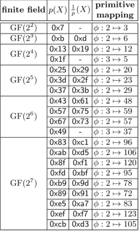
We programmed a tool that computes the XOR count for every nonzero element over GF(2r) forr= 2, . . . ,8 and for all possible irreducible polynomials (all the tables will be given in the full version of this article, we provide an extract in Appendix F). By analyzing the outputs of this tool, we could make two observations that are important to understand how the choice of the irreducible polynomial affects the XOR count. Before presenting our observations, we state some terminologies and properties related to reciprocal polynomials in finite fields.
Definition 2 A reciprocal polynomial 1p(X)of a polynomialp(X)overGF(2r), is a polynomial expressed as 1p(X) =Xr·p(X−1). A reciprocal finite field, K= GF(2r)/1
p(X), is a finite field defined by the reciprocal polynomial which defines F= GF(2r)/p(X).
In other words, a reciprocal polynomial is a polynomial with the order of the coefficients reversed. For example, the reciprocal polynomial of p(X) = 0x11b in GF(28) is 1
p(X) = 0x
1
11b =0x1b1. It is also to be noted that the reciprocal
polynomial of an irreducible polynomial is also irreducible.
The total XOR count. Our first new observation is that even if for an indi-vidual element of the field the choice of the irreducible polynomial has an impact on the XOR count, the total sum of the XOR count over all elements in the field is independent of this choice. We state this in the following theorem, the proof being provided in Appendix D.1.
Theorem 1 The total XOR count for a fieldGF(2r)isrPr i=22
i−2(i−1), where
r≥2.
From Theorem 1, it seems that there is no clear implication that one irre-ducible polynomial is strictly better than another, as the mean XOR count is the same for any irreducible polynomial. However, the irreducible polynomials have different distribution of the XOR count among the field elements, that is quantified by the standard deviation. A high standard deviation implies that the distribution of XOR count is very different from the mean, thus there will be more elements with relatively lower/higher XOR count. In general, the order of the finite field is much larger than the order of the MDS matrix and since only a few elements of the field will be used in the MDS matrices, there is a better chance of finding an MDS matrix with lower XOR count.
Hence, our recommendation is to choose the irreducible polynomial with the highest standard deviation regarding the XOR count distribution. From previous example, in GF(24) (XOR count mean equals 4.25 for this field dimension), the irreducible polynomials0x13and0x19lead to a standard deviation of 2.68, while
0x1f leads to a standard deviation of 1.7075. Therefore, the two first polynomials seem to be a better choice. This observation will allow us to choose the best irreducible polynomial to start with during the searches. We refer to Appendix F for all the standard deviations according to the irreducible polynomial.
We note that the folklore belief was that in order to get lightweight imple-mentations, one should use a low Hamming weight irreducible polynomial. The underlying idea is that with such a polynomial less XORs might be needed when the modular reduction has to be applied during a field multiplication. However, we have shown that this is not necessarily true. Yet, by looking at the data from Appendix F, we remark that the low Hamming weight irreducible polynomials usually have a high standard deviation, which actually validates the folklore be-lief. We conjecture that this heuristic will be less and less exact when we go to higher and higher order fields.
Matching XOR count. Our second new observation is that the XOR count distribution implied by a polynomial will be the same compared to the distri-bution of its reciprocal counterpart. We state this observation in the following theorem, the proof being provided in Appendix D.2.
Theorem 2 There exists an isomorphic mapping from a primitiveα∈GF(2r)/p(X) to another primitive β ∈ GF(2r)/1
p(X) where the XOR count of α
i and βi is equal for eachi={1,2, ...,2r−1}.
In Appendix E, we listed all the primitive mapping from a finite field to its re-ciprocal finite field for all fields GF(2r) withr= 2, . . . ,8 and for all possible irre-ducible polynomials. We give an example to illustrate our theorem. For GF(24), there are three irreducible polynomials:0x13,0x19and0x1fand the XOR count for the elements are shown in Appendix F. From the binary representation we see that 0x131 = 0x19. Consider an isomorphic mapping φ : GF(24)/0x13 →
GF(24)/0x19 defined as φ(2) = 12, where 2 and 12 are the primitives for the respective finite fields. Table 2 of Appendix E shows that the order of the XOR count is the same.
We remark that for a self-reciprocal irreducible polynomial, for instance0x1f in GF(24), there also exists an automorphism mapping from a primitive to an-other primitive with the same order of XOR count (see Appendix E).
Theorem 2 is useful for understanding that we do not need to consider GF(2r)/1p(X) when we are searching for lightweight matrices. As there exists an isomorphic mapping preserving the order of the XOR count, any MDS matrix over GF(2r)/1
p(X) can be mapped to an MDS matrix over GF(2
r)/p(X) while preserving the XOR count. Therefore, it is redundant to search for lightweight MDS matrices over GF(2r)/1
p(X) as the lightest MDS matrix can also be found in GF(2r)/p(X). This will render our algorithms much more efficient: when using exhaustive search for low XOR count MDS over finite field defined by various irreducible polynomial, one can reduce the search space by almost a factor 2 as the reciprocal polynomials are redundant.
3
Types of MDS matrices and properties
In this section, we first recall a few properties of MDS matrices and we then explain various constructions of (involutory) MDS matrices that were used to generate lightweight candidates. Namely, we will study 4 types of diffusion matri-ces: circulant, Hadamard, Cauchy, and Hadamard-Cauchy. We recall that we do not consider serially computable matrices in this article, like the ones described in [18, 19, 28, 32, 3, 2], since they are not adapted to round-based implementa-tions. As MDS matrices are widely studied and their properties are commonly known, their definition and properties are given in the Appendix A.
3.1 Circulant matrices
A common way to build an MDS matrix is to start from a circulant matrix, reason being that the probability of finding an MDS matrix would then be higher than a normal square matrix [16].
Definition 3 A k×k matrixC is circulant when each row vector is rotated to the right relative to the preceding row vector by one element. The matrix is then fully defined by its first row.
An interesting property of circulant matrices is that since each row differs from the previous row by a right shift, a user can just implement one row of the matrix multiplication in hardware and reuse the multiplication circuit for subsequent rows by just shifting the input. However in this paper, we will show in Section B.1 and C.1 that these matrices are not the best choice.
3.2 Hadamard matrices
Definition 4 ([20]) A finite field Hadamard (or simply called Hadamard) ma-trix H is a k×k matrix, with k = 2s, that can be represented by two other submatricesH1 andH2 which are also Hadamard matrices:
H = H1H2 H2H1 .
Similarly to [20], in order to represent a Hadamard matrix we use notation
had(h0, h1, ..., hk−1) (with hi =H[0, i] standing for the entries of the first row of the matrix) where H[i, j] = hi⊕j and k = 2s. It is clear that a Hadamard matrix is bisymmetric. Indeed, if we define the left and right diagonal reflection transformations as HL =TL(H) and HR = TR(H) respectively, we have that
HL[i, j] =H[j, i] =H[i, j] andHR[i, j] =H[k−1−i, k−1−j] =H[i, j] (the binary representation ofk−1 = 2s−1 is all 1, hencek−1−i= (k−1)⊕i).
Moreover, by doing the multiplication directly, it is known that if H =
h2
0+h21+h22+...+h2k−1. In other words, the product of a Hadamard matrix with itself is a multiple of an identity matrix, where the multiple c2 is the sum of the square of the elements from the first row.
A direct and crucial corollary to this fact is that a Hadamard matrix over GF(2r) is involution if the sum of the elements of the first row is equal to 1. Now, it is important to note that if one deals with a Hadamard matrix for which the sum of the first row over GF(2r) is nonzero, we can very simply make it involutory by dividing it with the sum of its first row.
We will use these considerations in Section B.2 to generate low dimension diffusion matrices (order 4 and 8) with an innovative exhaustive search over all the possible Hadamard matrices. We note that, similarity to a circulant matrix, an Hadamard matrix will have the interesting property that each row is a per-mutation of the first row, therefore allowing to reuse the multiplication circuit to save implementation costs.
3.3 Cauchy matrices
Definition 5 A square Cauchy matrix,C, is ak×kmatrix constructed with two disjoint sets of elements from GF(2r), {α
0, α1, ..., αk−1} and {β0, β1, ..., βk−1} such that C[i, j] = α 1
i+βj.
It is known that the determinant of a square Cauchy matrix,C, is given as
det(C) = Q 0≤i<j≤k−1(αj−αi)(βj−βi) Q 0≤i<j≤k−1(αi+αj) .
Sinceαi6=αj,βi 6=βjfor alli, j∈ {0,1, ..., k−1}, a Cauchy matrix is nonsingu-lar. Note that for a Cauchy matrix over GF(2r), the subtraction is equivalent to addition as the finite field has characteristic 2. As the sets are disjoint, we have
αi6=βj, thus all entries are well-defined and nonzero. In addition, any submatrix of a Cauchy matrix is also a Cauchy matrix as it is equivalent to constructing a smaller Cauchy matrix with subsets of the two disjoint sets. Therefore, by the first statement of Proposition 3, a Cauchy matrix is an MDS matrix.
3.4 Hadamard-Cauchy matrices
The innovative exhaustive search over Hadamard matrices from Section B.2 is sufficient to generate low dimension diffusion matrices (order 4 and 8). However, the computation for verifying the MDS property and the exhaustive search space grows exponentially. It eventually becomes impractical to search for higher di-mension Hadamard matrices (order 16 or more). Therefore, we use the Hadamard-Cauchy matrix construction, proposed in [20] as an evolution of the involutory MDS Vandermonde matrices [28], that guarantees the matrix to be an involutory MDS matrix.
In [20], the authors proposed a 2s×2smatrix construction that combines both the characteristics of Hadamard and Cauchy matrices. Because it is a Cauchy matrix, a Hadamard-Cauchy matrix is an MDS matrix. And because it is a Hadamard matrix, it will be involutory whenc2 is equal to 1. Therefore, we can construct a Hadamard-Cauchy matrix and check if the sum of first row is equal to 1 and, if so, we have an MDS and involutory matrix. A detailed discussion on Hadamard-Cauchy matrices is given in Section B.3.
4
Equivalence classes of Hadamard-based matrices
Our methodology for finding lightweight MDS matrices is to perform an inno-vative exhaustive search and by eventually picking the matrix with the lowest XOR count. Naturally, the main problem to tackle is the huge search space. By exploiting the properties of Hadamard matrices, we found ways to group them in equivalent classes and significantly reduce the search space. In this section, we introduce the equivalence classes of Hadamard matrices and the equivalence classes of involutory Hadamard-Cauchy matrices. It is important to note that these two equivalence classes are rather different as they are defined by very dif-ferent relations. We will later use these classes in Sections B.2, B.3, C.2 and C.3.
4.1 Equivalence classes of Hadamard matrices
It is known that a Hadamard matrix can be defined by its first row, and different permutation of the first row results in a different Hadamard matrix with possibly different branch number. In order to find a lightweight MDS involution matrix, it is necessary to have a set of k elements with relatively low XOR count that sum to 1 (to guarantee involution). Moreover, we need all coefficients in the first row to be different. Indeed, if the first row of an Hadamard matrix has 2 or more of the same element, say H[0, i] =H[0, j], where i, j ∈ {0,1, ..., k−1}, then in another row we haveH[i⊕j, i] =H[i⊕j, j]. These 4 entries are the same and by Corollary 3, H is not MDS.
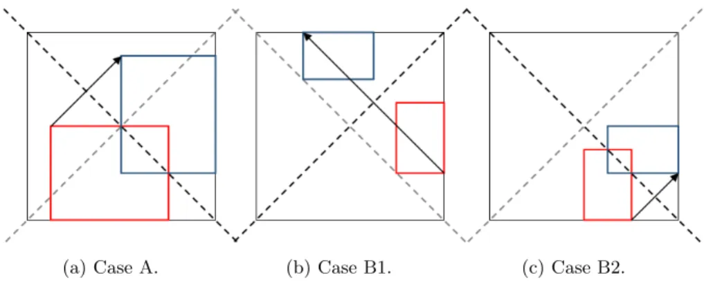
By permuting the entries we hope to find an MDS involution matrix. How-ever, givenk distinct nonzero elements, there are k! ways to permute the first row of the Hadamard matrix, which can quickly become intractable. Therefore, we introduce a relation that relates certain permutations that lead to the same branch number.
Definition 6 Let H andH(σ) be two Hadamard matrices with the same set of entries up to some permutation σ. We say that they are related, H ∼H(σ), if every pair of input vectors,(v, v(σ))with the same permutationσ, toH andH(σ) respectively, have the same set of elements in the output vectors.
For example, let us consider the following three Hadamard matrices H = w x y z x w z y y z w x z y x w , H(σ1)= y z w x z y x w w x y z x w z y , H(σ2)= w x z y x w y z z y w x y z x w ,
One can see thatH(σ1)is defined by the third row ofH, i.e. the rows are shifted
by two positions andσ1={2,3,0,1}. Let us consider an arbitrary input vector for H, say v = (a, b, c, d). Then, if we apply the permutation to v, we obtain
v(σ1)= (c, d, a, b). We can observe that:
v·H = (aw+bx+cy+dz, ax+bw+cz+dy, ay+bz+cw+dx, az+by+cx+dw), v(σ1)·H(σ1)= (cy+dz+aw+bx, cz+dy+ax+bw, cw+dx+ay+bz, cx+dw+az+by),
It is now easy to see thatv·H =v(σ1)·H(σ1). Hence, we say that H ∼H(σ1).
Similarily, withσ2={0,1,3,2}, we havev(σ2)= (a, b, d, c) and:
v·H = (aw+bx+cy+dz, ax+bw+cz+dy, ay+bz+cw+dx, az+by+cx+dw), v(σ2)·H(σ2)= (aw+bx+dz+cy, ax+bw+dy+cz, az+by+dw+cx, ay+bz+dx+cw),
and sincev·H andv(σ2)·H(σ2) are the same up to the permutationσ
2, we can say thatH ∼H(σ2).
Definition 7 An equivalence class of Hadamard matrices is a set of Hadamard matrices satisfying the equivalence relation ∼.
Proposition 1 Hadamard matrices in the same equivalence class have the same branch number.
When searching for an MDS matrix, we can make use of this property to greatly reduce the search space: if one Hadamard matrix in an equivalence class is not MDS, then all other Hadamard matrices in the same equivalence class will not be MDS either. Therefore, it all boils down to analyzing how many and which permutation of the Hadamard matrices belongs to the same equivalence classes. Using the two previous examples σ1 and σ2 as building blocks, we generalize them and present two lemmas.
Lemma 1 Given a Hadamard matrix H, any Hadamard matrix H(α) defined by the(α+ 1)-th row of H, with α= 0,1,2, ..., k−1, is equivalent toH.
Next, let us consider the other type of permutation. We can see in the example with σ2 that up to the permutation applied to the Hadamard matrix, input and output vectors are the same. LetH(σ), v(σ)and u(σ) denote the permuted Hadamard matrix, the permuted input vector and its corresponding permuted output vector. We want the permutation to satisfy uσ(j) = u
(σ)
j , where j ∈
as the permuted output vector of H(σ). Using the definition of the Hadamard matrix, we can rewrite it as
k−1 M i=0 vihi⊕σ(j)= k−1 M i=0 v(iσ)H(σ)[i, j].
Using the definition of the permutation and by the fact that it is one-to-one mapping, we can rearrange the XOR order of the terms on the left-hand side and we obtain k−1 M i=0 vσ(i)hσ(i)⊕σ(j)= k−1 M i=0 vσ(i)hσ(i⊕j).
Therefore, we need the permutation to be linear with respect to XOR:σ(i⊕j) =
σ(i)⊕σ(j). This proves our next lemma.
Lemma 2 For any linear permutationσ (w.r.t. XOR), the two Hadamard ma-tricesH andH(σ) are equivalent.
We note that the permutations in Lemma 1 and 2 are disjoint, except for the identity permutation. This is because for the linear permutationσ, it always maps the identity to itself: σ(0) = 0. Thus, for any linear permutation, the first entry remains unchanged. On the other hand, when choosing another row ofH
as the first row, the first entry is always different.
With these two lemmas, we can now partition the family of Hadamard ma-trices into equivalence classes. For Lemma 1, we can easily see that the number of permutation is equal to the order of the Hadamard matrix. However, for Lemma 2 it is not so trivial. Therefore, we have the following lemma.
Lemma 3 Given a set of 2s nonzero elements, S = {α
0, α1, ..., α2s−1}, there
are Qs−1 i=0(2
s−2i)linear permutations w.r.t. XOR operation. Theorem 3 Given a set of2s nonzero elements,S ={α
0, α1, ..., α2s−1}, there
are Qs(2−1s−1)!
i=0(2s−2i)
equivalence classes of Hadamard matrices of order2s defined by the set of elementsS.
For convenience, we call the permutations in Lemma 1 and 2 theH-permutations. The H-permutations can be described as a sequence of the following types of permutations on the index of the entries:
1. chooseα∈ {0,1, ...,2s−1}, defineσ(i) =i⊕α,∀i= 0,1, ...,2s−1, and 2. fixσ(0) = 0, in ascending order of the indexi, choose the permutation ifiis
power of 2, otherwise it is defined by the linear permutation (w.r.t. XOR):
σ(i⊕j) =σ(i)⊕σ(j).
We remark that given a set of 4 nonzero elements, from Theorem 3 we see that there is only 1 equivalence class of Hadamard matrices. This implies that
there is no need to permute the entries of the 4×4 Hadamard matrix in hope to find MDS matrix if one of the permutation is not MDS.
With the knowledge of equivalence classes of Hadamard matrices, what we need is an algorithm to pick one representative from each equivalence class and check if it is MDS. The idea is to exhaust all non-H-permutations through select-ing the entries in ascendselect-ing index order. Since the entries in the first column of Hadamard matrix are distinct (otherwise the matrix is not MDS), it is sufficient for us to check the matrices with the first entry (index 0) being the smallest element. This is because for any other matrices with the first entry set as some other element, it is in the same equivalence class as some matrix H(α) where the first entry of (α+ 1)-th row is the smallest element. For indexes that are powers of 2, select the smallest element from the remaining set. While for the other entries, one can pick any element from the remaining set.
For 8×8 Hadamard matrices for example, the first three entries, α0, α1 and α2 are fixed to be the three smallest elements in ascending order. Next, by Lemma 2,α3 should be defined byα1andα2 in order to preserve the linear property, thus to ”destroy” the linear property and obtain matrices from different equivalence classes, pick an element from the remaining set in ascending order as the fourth entry α3. After which, α4 is selected to be the smallest element among the remaining 4 elements and permute the remaining 3 elements to beα5,
α6andα7respectively. For each of these arrangement of entries, we check if it is MDS using the algorithm discussed in Section B.2. We terminate the algorithm prematurely once an MDS matrix is found, else we conclude that the given set of elements does not generate an MDS matrix.
It is clear that arranging the entries in this manner will not obtain two Hadamard matrices from the same equivalence class. But one may wonder if it actually does exhaust all the equivalence classes. The answer is yes: Theorem 3 shows that there is a total of 30 equivalence classes for 8×8 Hadamard matrices. On the other hand, from the algorithm described above, we have 5 choices for
α3and we permute the remaining 3 elements forα5,α6 andα7. Thus, there are 30 Hadamard matrices that we have to check.
4.2 Equivalence classes of involutory Hadamard-Cauchy matrices Despite having a new technique to reduce the search space, the computation cost for checking the MDS property is still too huge when the order of the Hadamard matrix is larger than 8. Therefore, we use the Hadamard-Cauchy construction for order 16 and 32. Thanks to the Cauchy property, we are ensured that the matrix will be MDS. Hence, the only problem that remains is the huge search space of possible Hadamard-Cauchy matrices. To prevent confusion with Hadamard matrices, we denote Hadamard-Cauchy matrices withK.
First, we restate in Algorithm 1 the technique from [20] to build involutory MDS matrices, with some modifications on the notations for the variables. Al-though it is not explicitly stated, we can infer from Lemma 6,7 and Theorem 4
from [20] that all Hadamard-Cauchy matrices can be expressed as an output of Algorithm 1.
Algorithm 1 Construction of 2s×2s MDS matrix or involutory MDS matrix over GF(2r)/p(X).
INPUT: an irreducible polynomialp(X) of GF(2r), integerss, rsatisfyings < rand
r >1, a booleanBinvolutory.
OUTPUT: 2s×2sHadamard-Cauchy matrixK, whereKis involutory ifB
involutory is setTrue.
procedureConstructH-C(r, p(X), s, Binvolutory)
selectslinearly independent elementsx1, x2, x22, ..., x2s−1 from GF(2r) and
con-structS, the set of 2selementsxi,
wherexi=Lt=0s−1btx2t for alli∈[0,2s−1] (with (bs−1, bs−2, ..., b1, b0) being the binary representation ofi)
selectz∈GF(2r)\S and construct the set of 2s elementsyi, whereyi=z+xi
for alli∈[0,2s−1]
initialize an empty arrayary sof size 2s
if (Binvolutory==False)then
ary s[i] = 1 yi for alli∈[0,2 s−1] else ary s[i] = 1 c·yi for alli∈[0,2 s−1], wherec=Ls−1 t=0 1 z+xt end if
construct the 2s×2s matrixK, whereK[i, j] =ary s[i⊕j]
returnK end procedure
Similarly to Hadamard matrices, we denote a Hadamard-Cauchy matrix by its first row of elements as hc(h0, h1, ..., h2s−1), with hi = K[0, i]. To summa-rize the construction of a Hadamard-Cauchy matrix of order 2s mentioned in Algorithm 1, we pick an ordered set ofs+ 1 linearly independent elements, we call it the basis. We use the first s elements to span an ordered set S of 2s elements, and add the last elementzto all the elements inS. Next, we take the inverse of each of the elements in this new set and we get the first row of the Hadamard-Cauchy matrix. Lastly, we generate the matrix based on the first row in the same manner as an Hadamard matrix.
For example, for an 8×8 Hadamard-Cauchy matrix over GF(24)/0x13, say we choose x1 = 1, x2 = 2, x4 = 4, we generate the setS ={0,1,2,3,4,5,6,7}, choosingz= 8 and taking the inverses in the new set, we get a Hadamard-Cauchy matrix K = hc(15,2,12,5,10,4,3,8). To make it involution, we multiply each element by the inverse of the sum of the elements. However for this instance the sum is 1, henceK is already an involutory MDS matrix.
One of the main differences between the Hadamard and Hadamard-Cauchy matrices is the choice of entries. While we can choose all the entries for a
Hadamard matrix to be lightweight and permute them in search for an MDS candidate, the construction of Hadamard-Cauchy matrix makes it nontrivial to control its entries efficiently. Although in [20] the authors proposed a backward re-construction algorithm that finds a Hadamard-Cauchy matrix with some pre-decided lightweight entries, the number of entries that can be pre-decided beforehand is very limited. For example, for a Hadamard-Cauchy matrix of order 16, the algorithm can only choose 5 lightweight entries, the weight of the other 11 entries is not controlled. The most direct way to find a lightweight Hadamard-Cauchy matrix is to apply Algorithm 1 repeatedly for all possible basis. We introduce now new equivalence classes that will help us to exhaust all possible Hadamard-Cauchy matrices with much lesser memory space and number of iterations. Definition 8 Let K1 and K2 be two Hadamard-Cauchy matrices, we say they are related,K1∼HC K2, if one can be transformed to the other by either one or both operations on the first row of entries:
1. multiply by a nonzero scalar, and 2. H-permutation of the entries.
The crucial property of the construction is the independence of the elements in the basis, which is not affected by multiplying a nonzero scalar. Hence, we can convert any Hadamard-Cauchy matrix to an involutory Hadamard-Cauchy ma-trix by multiplying it with the inverse of the sum of the first row and vice versa. However, permutating the positions of the entries is the tricky part. Indeed, for the Hadamard-Cauchy matrices of order 8 or higher, some permutations destroy the Cauchy property, causing it to be non-MDS. Using our previous 8×8 ex-ample, suppose we swap the first two entries,K0 =hc(2,15,12,5,10,4,3,8), it can be verified that it is not MDS. To understand why, we work backwards to find the basis corresponding to K0. Taking the inverse of the entries, we have
{9,8,10,11,12,13,14,15}. However, there is no basis that satisfies the 8 linear equations for the entries. Thus it is an invalid construction of Hadamard-Cauchy matrix. Therefore, we consider applying theH-permutation on Hadamard-Cauchy matrix. Since it is also a Hadamard matrix, the H-permutation preserves its branch number, thus it is still MDS. So we are left to show that a Hadamard-Cauchy matrix that undergoesH-permutation is still a Hadamard-Cauchy ma-trix.
Lemma 4 Given a 2s×2s involutory Hadamard-Cauchy matrix K, there are 2s·Qs−1
i=0(2
s−2i) involutory Hadamard-Cauchy matrices that are related toK by theH-permutations of the entries of the first row.
With that, we can define our equivalence classes of involutory Hadamard-Cauchy matrices.
Definition 9 An equivalence class of involutory Hadamard-Cauchy matrices is a set of Hadamard-Cauchy matrices satisfying the equivalence relation ∼HC.
In order to count the number of equivalence classes of involutory Hadamard-Cauchy matrices, we use the same technique for proving Theorem 3. To do that, we need to know the total number of Hadamard-Cauchy matrices that can be constructed from the Algorithm 1 for a given finite field.
Lemma 5 Given two natural numberssandr, based on Algorithm 1, there are Qs
i=0(2
r−2i)many2s×2sHadamard-Cauchy matrices overGF(2r).
Theorem 4 Given two positive integerssandr, there areQs−1 i=0
2r−1−2i
2s−2i
equiva-lence classes of involutory Hadamard-Cauchy matrices of order2soverGF(2r). In [15], the authors introduced the notion of compact Cauchy matrices which are defined as Cauchy matrices with exactly 2sdistinct elements. These matrices seem to include Cauchy matrices beyond the class of Hadamard-Cauchy matri-ces. However, it turns out that the equivalence classes of involutory Hadamard-Cauchy matrices can be extended to compact Hadamard-Cauchy matrices.
Corollary 1 Any compact Cauchy matrices can be generated from some equiv-alence class of involutory Hadamard-Cauchy matrices.
Note that since the permutation of the elements inS andz+S only results in rearrangement of the entries of the compact Cauchy matrix, the XOR count is invariant from Hadamard-Cauchy matrix with the same set of entries.
5
Searching for involutory MDS and non-involutory
MDS matrices
Due to space constraints, we have put respectively in Appendix B and C the new methods we have designed to look for the lightest possible involutory MDS and non-involutory MDS matrices.
More precisely, regarding involutory MDS matrices (see Appendix B), using the previous properties and equivalence classes given in Sections 3 and 4 for several matrix constructions, we have derived algorithms to search for the most lightweight candidate. First, we point out that the circulant construction can not lead to involutory MDS matrices, then we focus on the case of matrices of small dimension using the Hadamard construction. For bigger dimension, we add the Cauchy property to the Hadamard one in order to guarantee that the matrix will be MDS. We recall that, similarity to a circulant matrix, an Hadamard matrix will have the interesting property that each row is a permutation of the first row, therefore allowing to reuse the multiplication circuit to save implementation costs.
Regarding non-involutory MDS matrices (see Appendix C), we have extended the involutory MDS matrix search to include non-involutory candidates. For
Hadamard construction, we removed the constraint that the sum of the first row elements must be equal to 1. For the Hadamard-Cauchy, we multiply each equivalent classes by a non-zero scalar value. We note that the disadvantage of non-involutory MDS matrices is that their inverse may have a high computation cost. But if the inverse is not required (for example in the case of popular con-structions such as a Feistel network, or a CTR encryption mode), non-involution matrices might be lighter than involutory matrices.
6
Results
We first emphasize that although in [20, 15] the authors proposed methods to construct lightweight matrices, the choice of the entries are limited as mentioned in Section 4.2. This is due to the nature of the Cauchy matrices where the inverse of the elements are used during the construction, which makes it non-trivial to search for lightweight Cauchy matrices7. However, using the concept of equivalence classes, we can exhaust all the matrices and pick the lightest-weight matrix.
We applied the algorithms of Section 5 to construct lightweight MDS in-volutions over GF(28). We list them in the upper half of Table 1 and we can see that they are much lighter than known MDS involutions like the KHAZAD and ANUBIS, previous Hadamard-Cauchy matrices [6, 20] and compact Cauchy matrices [15]. In lower half of Table 1, we list the GF(28) MDS matrices we found using the methods of Appendix C and show that they are lighter than known MDS matrices like the AES, WHIRLPOOL and WHIRLWIND matrices [17, 8, 7]. We also compare with the 14 lightweight candidate matrices C0 to C13 for theWHIRLPOOLhash functions suggested during the NESSIE workshop [30, Sec-tion 6]. Table 1 is comparing our matrices with the ones explicitly provided in the previous articles. Recently, Guptaet al.[21] constructed some circulant matrices that is lightweight for both itself and its inverse. However we do not compare them in our table because their approach minimizes the number of XORs, look-up tables and temporary variables, which might be optimal for software but not for hardware implementations based purely on XOR count.
By Theorem 2 in Section 2, we only need to apply the algorithms from Section 5 for half the representations of GF(28) when searching for optimal lightweight matrices. And as predicted by the discussion after Theorem 1, the lightweight matrices we found in Table 1 do come from GF(28) representations with higher standard deviations.
We provide in the first column of the Table 1 the type of the matrices. They can be circulant, Hadamard or Cauchy-Hadamard. The subfield-Hadamard con-struction is based on the method of [24, Section 7.2] which we explain here.
7
Using direct construction, there is no clear implication for the choice of the ele-mentsαiandβjthat will generate lightweight entriescij. On the other hand, every lightweight entry chosen beforehand will greatly restrict the choices for the remaining entries if one wants to maintain two disjoint sets of elements{αi}and{βj}.
Consider the MDS involution M = had(0x1,0x4,0x9,0xd) over GF(24)/0x13 in the first row of Table 1. Using the method of [24, Section 7.2], we can ex-tend it to a MDS involution over GF(28) by using two parallel copies of Q. The matrix is formed by writing each input bytexj as a concatenation of two nibblesxj = (xLj||xRj). Then the MDS multiplication is computed on each half (yL
1, yL2, y3L, yL4) =M·(xL1, xL2, xL3, xL4) and (yR1, yR2, y3R, yR4) =M·(xR1, xR2, xR3, xR4) over GF(24). The result is concatenated to form four output bytes (y
1, y2, y3, y4) whereyj= (yjL||yjR).
We could have concatenated different submatrices and this is done in the WHIRLWIND hash function [7], where the authors concatenated four MDS sub-matrices over GF(24) to form (M
0|M1|M1|M0), an MDS matrix over GF(216). The submatrices are non-involutory Hadamard matricesM0=had(0x5,0x4,0xa, 0x6,0x2,0xd,0x8,0x3) andM1= (0x5,0xe,0x4,0x7,0x1,0x3,0xf,0x8) defined over GF(24)/0x13. For fair comparison with our GF(28) matrices in Table 1, we con-sider the correspondingWHIRLWIND-like matrix (M0|M1) over GF(28) which takes half the resource of the originalWHIRLWINDmatrix and is also MDS.
The second column of the result tables gives the finite field over which the matrix is defined, while the third column displays the first row of the matrix where the entries are bytes written in hexadecimal notation. The fourth column gives the XOR count to implement the first row of the n×n matrix. Because all subsequent rows are just permutations of the first row, the XOR count to implement the matrix is just n times this number. For example, to compute the XOR count for implementing had(0x1,0x4,0x9,0xd) over GF(24)/0x13, we consider the expression for the first row of matrix multiplication0x1·x1⊕0x4·x2⊕ 0x9·x3⊕0xd·x4. From Table 4 of Appendix F, the XOR count of multiplication by 0x1,0x4,0x9 and 0xd are 0, 2, 1 and 3, which gives us a cost of (0 + 2 + 1 + 3) + 3×4 = 18 XORs to implement one row of the matrix (the summand 3×4 account for the three XORs summing the four nibbles). For the subfield construction over GF(28), we need two copies of the matrix giving a cost of 18×2 = 36 XORs to implement one row.
Due to page constraints, we only give comparisons with known lightweight matrices over GF(28). The comparisons with GF(24) matrices will be provided in the full version of the paper. In fact, the subfield-Hadamard constructions in Table 1 already captures lightweight GF(24) matrices, and we show that our construction are lighter than known ones. For example in the lower half of Ta-ble 1, the GF(24) matricesM
0andM1used in theWHIRLWINDhash function has XOR count 61 and 67 respectively while our Hadamard matrixhad(0x1,0x2,0x6, 0x8,0x9,0xc,0xd,0xa) has XOR count 54.
With our work, we can now see that one can use involutory MDS for almost the same price as non-involutory MDS. For example in the upper half of Table 1, the previous 4×4 MDS involution from [20] is about 3 times heavier than theAES matrix8; but in this paper, we have used an improved search technique to find
8
We acknowledge that there are implementations that requires lesser XOR to imple-ment directly the entire circulantAES matrix. However, the small savings obtained
an MDS involution lighter than theAESand ANUBISmatrix. Similarly, we have found 8×8 MDS involutions which are much lighter than theKHAZADinvolution matrix, and even lighter than lightweight non-involutory MDS matrix like the WHIRLPOOL matrix. Thus, our method will be useful for future construction of lightweight ciphers based on involutory components like the ANUBIS, KHAZAD, ICEBERGandPRINCEciphers.
on XOR count are completely outweighed by the extra memory cost required for such an implementation in terms of temporary variables.
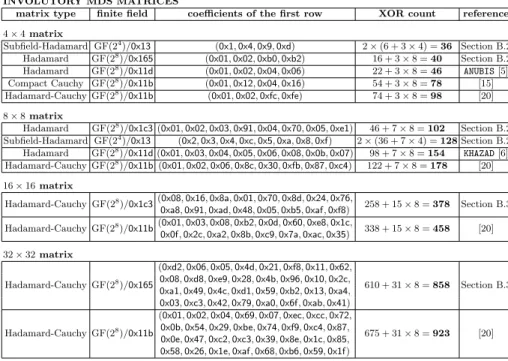
Table 1:Comparison of MDS Matrices over GF(28). The upper table compares the involutory MDS matrices, while the lower table compares the non-involutory MDS matrices (the factor 2 is due to the fact that we have to implement two copies of the
matrices) INVOLUTORY MDS MATRICES
matrix type finite field coefficients of the first row XOR count reference
4×4matrix Subfield-Hadamard GF(24)/0x13 (0x1,0x4,0x9,0xd) 2×(6 + 3×4) =36 Section B.2 Hadamard GF(28)/0x165 (0x01,0x02,0xb0,0xb2) 16 + 3×8 =40 Section B.2 Hadamard GF(28)/0x11d (0x01,0x02,0x04,0x06) 22 + 3×8 =46 ANUBIS[5] Compact Cauchy GF(28)/0x11b (0x01,0x12,0x04,0x16) 54 + 3×8 =78 [15] Hadamard-Cauchy GF(28)/0x11b (0x01,0x02,0xfc,0xfe) 74 + 3×8 =98 [20] 8×8matrix
Hadamard GF(28)/0x1c3(0x01,0x02,0x03,0x91,0x04,0x70,0x05,0xe1) 46 + 7×8 =102 Section B.2
Subfield-Hadamard GF(24)/0x13 (0x2,0x3,0x4,0xc,0x5,0xa,0x8,0xf) 2×(36 + 7×4) =128Section B.2
Hadamard GF(28)/0x11d(0x01,0x03,0x04,0x05,0x06,0x08,0x0b,0x07) 98 + 7×8 =154
KHAZAD[6] Hadamard-Cauchy GF(28)/0x11b(0x01,0x02,0x06,0x8c,0x30,0xfb,0x87,0xc4) 122 + 7×8 =178 [20]
16×16matrix
Hadamard-Cauchy GF(28)/0x1c3(0x08,0x16,0x8a,0x01,0x70,0x8d,0x24,0x76, 258 + 15×8 =378 Section B.3 0xa8,0x91,0xad,0x48,0x05,0xb5,0xaf,0xf8)
Hadamard-Cauchy GF(28)/0x11b(0x01,0x03,0x08,0xb2,0x0d,0x60,0xe8,0x1c, 338 + 15×8 =458 [20] 0x0f,0x2c,0xa2,0x8b,0xc9,0x7a,0xac,0x35)
32×32matrix Hadamard-Cauchy GF(28)/0x165 (0xd2,0x06,0x05,0x4d,0x21,0xf8,0x11,0x62, 610 + 31×8 =858 Section B.3 0x08,0xd8,0xe9,0x28,0x4b,0x96,0x10,0x2c, 0xa1,0x49,0x4c,0xd1,0x59,0xb2,0x13,0xa4, 0x03,0xc3,0x42,0x79,0xa0,0x6f,0xab,0x41) Hadamard-Cauchy GF(28)/0x11b (0x01,0x02,0x04,0x69,0x07,0xec,0xcc,0x72, 675 + 31×8 =923 [20] 0x0b,0x54,0x29,0xbe,0x74,0xf9,0xc4,0x87, 0x0e,0x47,0xc2,0xc3,0x39,0x8e,0x1c,0x85, 0x58,0x26,0x1e,0xaf,0x68,0xb6,0x59,0x1f) NON-INVOLUTORY MDS MATRICES
matrix type finite field coefficients of the first row XOR count reference
4×4matrix Subfield-Hadamard GF(24)/0x13 (0x1,0x2,0x8,0x9) 2×(5 + 3×4) =34 Section C.2 Hadamard GF(28)/0x1c3 (0x01,0x02,0x04,0x91) 13 + 3×8 =37 Section C.2 Circulant GF(28)/0x11b (0x02,0x03,0x01,0x01) 14 + 3×8 =38 AES[17] 8×8matrix
Hadamard GF(28)/0x1c3(0x01,0x02,0x03,0x08,0x04,0x91,0xe1,0xa9) 40 + 7×8 =96 Section C.2
Circulant GF(28)/0x11d(0x01,0x01,0x04,0x01,0x08,0x05,0x02,0x09) 49 + 7×8 =105
WHIRLPOOL[8] Subfield-Hadamard GF(24)/0x13 (0x1,0x2,0x6,0x8,0x9,0xc,0xd,0xa) 2×(26 + 7×4) =108 Section C.2
Circulant GF(28)/0x11d
WHIRLPOOL-like matrices between105to117 [30] Subfield-Hadamard GF(24)/0x13 WHIRLWIND-like matrix 33 + 39 + 2×7×4 =128 [7]
16×16matrix
Hadamard-Cauchy GF(28)/0x1c3(0xb1,0x1c,0x30,0x09,0x08,0x91,0x18,0xe4, 232 + 15×8 =352 Section C.3 0x98,0x12,0x70,0xb5,0x97,0x90,0xa9,0x5b) 32×32matrix Hadamard-Cauchy GF(28)/0x1c3 (0xb9,0x7c,0x93,0xbc,0xbd,0x26,0xfa,0xa9, 596 + 31×8 =844 Section C.3 0x32,0x31,0x24,0xb5,0xbb,0x06,0xa0,0x44,
0x95,0xb3,0x0c,0x1c,0x07,0xe5,0xa4,0x2e,
Acknowledgments
The authors would like to thank the anonymous referees for their helpful com-ments. We also wish to thank Wang HuaXiong for providing useful and valuable suggestions.
References
1. E. Andreeva, B. Bilgin, A. Bogdanov, A. Luykx, F. Mendel, B. Mennink, N. Mouha, Q. Wang, and K. Yasuda. PRIMATEs v1. Submission to the CAESAR Competi-tion, 2014. http://competitions.cr.yp.to/round1/primatesv1.pdf.
2. D. Augot and M. Finiasz. Direct Construction of Recursive MDS Diffusion Layers using Shortened BCH Codes. InFSE, LNCS, 2014. To appear.
3. Daniel Augot and Matthieu Finiasz. Exhaustive search for small dimension re-cursive MDS diffusion layers for block ciphers and hash functions. InISIT, pages 1551–1555, 2013.
4. Jean-Philippe Aumasson, Luca Henzen, Willi Meier, and Mar´ıa Naya-Plasencia. Quark: A Lightweight Hash. InCHES, pages 1–15, 2010.
5. P. Barreto and V. Rijmen. The Anubis Block Cipher. Submission to the NESSIE Project, 2000.
6. P. Barreto and V. Rijmen. The Khazad Legacy-Level Block Cipher. First Open NESSIE Workshop, 2000.
7. Paulo S. L. M. Barreto, Ventzislav Nikov, Svetla Nikova, Vincent Rijmen, and Elmar Tischhauser. Whirlwind: a new cryptographic hash function. Des. Codes Cryptography, 56(2-3):141–162, 2010.
8. Paulo S. L. M. Barreto and Vincent Rijmen. Whirlpool. InEncyclopedia of Cryp-tography and Security (2nd Ed.), pages 1384–1385. 2011.
9. Ray Beaulieu, Douglas Shors, Jason Smith, Stefan Treatman-Clark, Bryan Weeks, and Louis Wingers. The SIMON and SPECK Families of Lightweight Block Ci-phers. Cryptology ePrint Archive, Report 2013/404, 2013.
10. Thierry P. Berger. Construction of Recursive MDS Diffusion Layers from Gabidulin Codes. InINDOCRYPT, volume 8250 ofLNCS, pages 274–285. Springer, 2013. 11. A. Bogdanov, M. Knezevic, G. Leander, D. Toz, K. Varici, and I. Verbauwhede.
spongent: A Lightweight Hash Function. InCHES, pages 312–325, 2011.
12. Andrey Bogdanov, Lars R. Knudsen, Gregor Leander, Christof Paar, Axel Poschmann, Matthew J. B. Robshaw, Yannick Seurin, and C. Vikkelsoe. PRESENT: An Ultra-Lightweight Block Cipher. In Pascal Paillier and Ingrid Ver-bauwhede, editors,CHES, volume 4727 ofLNCS, pages 450–466. Springer, 2007. 13. J. Borghoff, A. Canteaut, T. G¨uneysu, E. B. Kavun, M. Knezevic, L. R. Knudsen,
G. Leander, V. Nikov, C. Paar, C. Rechberger, P. Rombouts, S. S. Thomsen, and T. Yal¸cin. PRINCE - A Low-Latency Block Cipher for Pervasive Computing Applications - Extended Abstract. InASIACRYPT, pages 208–225, 2012. 14. C. De Canni`ere, O. Dunkelman, and M. Knezevic. KATAN and KTANTAN - A
Family of Small and Efficient Hardware-Oriented Block Ciphers. InCHES, pages 272–288, 2009.
15. T. Cui, C.i Jin, and Z. Kong. On compact cauchy matrices for substitution-permutation networks. IEEE Transactions on Computers, 99(PrePrints):1, 2014. 16. Joan Daemen, Lars R. Knudsen, and Vincent Rijmen. The Block Cipher Square.
17. Joan Daemen and Vincent Rijmen. The Design of Rijndael: AES - The Advanced Encryption Standard. Springer, 2002.
18. Jian Guo, Thomas Peyrin, and Axel Poschmann. The PHOTON Family of Lightweight Hash Functions. InCRYPTO, pages 222–239, 2011.
19. Jian Guo, Thomas Peyrin, Axel Poschmann, and Matthew J. B. Robshaw. The LED Block Cipher. InCHES, pages 326–341, 2011.
20. Kishan Chand Gupta and Indranil Ghosh Ray. On Constructions of Involutory MDS Matrices. InAFRICACRYPT, pages 43–60, 2013.
21. Kishan Chand Gupta and Indranil Ghosh Ray. On Constructions of Circulant MDS Matrices for Lightweight Cryptography. InISPEC, pages 564–576, 2014. 22. Jorge Nakahara Jr. and lcio Abraho. A new involutory mds matrix for the aes. I.
J. Network Security, 9(2):109–116, 2009.
23. Pascal Junod and Serge Vaudenay. Perfect Diffusion Primitives for Block Ciphers. In Helena Handschuh and M. Anwar Hasan, editors,Selected Areas in Cryptogra-phy, volume 3357 ofLNCS, pages 84–99. Springer, 2004.
24. K. Khoo, T. Peyrin, A. Poschmann, and H. Yap. FOAM: Searching for Hardware-Optimal SPN Structures and Components with a Fair Comparison. In Crypto-graphic Hardware and Embedded Systems CHES 2014, volume 8731 of Lecture Notes in Computer Science, pages 433–450. Springer Berlin Heidelberg, 2014. 25. J´erˆome Lacan and J´erˆome Fimes. Systematic MDS erasure codes based on
Van-dermonde matrices. IEEE Communications Letters, 8(9):570–572, 2004.
26. S. Ling and C. Xing. Coding Theory: A First Course. Coding Theory: A First Course. Cambridge University Press, 2004.
27. F.J. MacWilliams and N.J.A. Sloane. The Theory of Error-Correcting Codes. North-holland Publishing Company, 2nd edition, 1986.
28. M. Sajadieh, M. Dakhilalian, H. Mala, and P. Sepehrdad. Recursive Diffusion Layers for Block Ciphers and Hash Functions. InFSE, pages 385–401, 2012. 29. M.i Sajadieh, M. Dakhilalian, H. Mala, and B. Omoomi. On construction of
in-volutory MDS matrices from Vandermonde Matrices in GF(2 q ). Des. Codes Cryptography, 64(3):287–308, 2012.
30. T. Shirai and K. Shibutani. On the diffusion matrix employed in the Whirlpool hashing function. NESSIE Phase 2 Report NES/DOC/EXT/WP5/002/1. 31. Fran¸cois-Xavier Standaert, Gilles Piret, Ga¨el Rouvroy, Jean-Jacques Quisquater,
and Jean-Didier Legat. ICEBERG : An Involutional Cipher Efficient for Block Encryption in Reconfigurable Hardware. InFSE, pages 279–299, 2004.
32. Shengbao Wu, Mingsheng Wang, and Wenling Wu. Recursive Diffusion Layers for (Lightweight) Block Ciphers and Hash Functions. InSelected Areas in Cryptogra-phy, volume 7707 ofLNCS, pages 355–371. Springer Berlin Heidelberg, 2013. 33. A. M. Youssef, S. Mister, and S. E. Tavares. On the Design of Linear
Transforma-tions for Substitution Permutation Encryption Networks. InWorkshop On Selected Areas in Cryptography, pages 40–48, 1997.
A
Maximum Distance Separable matrices
Maximum Distance Separable matrices are crucial components in cryptographic designs, as they ensure a perfect diffusion layer. Since we will search among many lightweight candidate matrices and only keep the MDS ones, we recall in this subsection a few definitions and properties regarding these mathematical objects. We denote byIk thek×kidentity matrix.
Definition 10 The branch number of a k×k matrix M over GF(2r) is the minimum number of nonzero entries in the input vector v and output vector
v·M = u (denoted wt(v) and wt(u) respectively), as we range over all v ∈
[GF(2r)]k− {0}. I.e. the branching number is equal to min
x6=0{wt(v) +wt(u)}, and when the optimal value k+ 1 is attained, we sayM is an MDS matrix.
Definition 11 A lengthn, dimensionkand distancedbinary linear code[n, k, d] is called a MDS code if the Singleton boundk=n−d+ 1 is met.
From [16, Section 4], we have the following proposition to relate an MDS matrix to a MDS code.
Proposition 2 Ak×kmatrixM is an MDS matrix if and only if the standard form generator matrix [Ik|M] generates a(2k, k, k+ 1)-MDS code.
There are various ways to verify if a matrix is MDS, in this paper we state two of the commonly used statements that can be used to identify MDS matrix.
Proposition 3 ([27], page 321, Theorem 8 - [26], page 53, Theorem 5.4.5) Given a k×k matrixM, it is an MDS matrix if and only if
1. every square submatrix (formed from anyi rows and anyicolumns, for any
i= 1,2, ..., k) ofM is nonsingular,
2. anyk columns of[Ik|M] are linearly independent.
The two following corollaries are directly deduced from the first statement of Proposition 3 when we consider submatrices of order 1 and 2 respectively.
Corollary 2 All entries of an MDS matrix are nonzero.
Corollary 3 Given ak×kmatrixM, if there exists pairwise distincti1, i2, j1, j2∈
{0,1, ..., k−1} such that M[i1, j1] =M[i1, j2] = M[i2, j1] = M[i2, j2], then M is not an MDS matrix.
B
Searching for MDS and involutory matrices
In this section, using the previous properties and equivalence classes given in Sections 3 and 4 for several matrix constructions, we will derive algorithms to search for lightweight involutory MDS matrices. First, we show that the circulant construction can not lead to such matrices, then we focus on the case of matri-ces of small dimension using the Hadamard construction. For bigger dimension, we add the Cauchy property to the Hadamard one in order to guarantee that the matrix will be MDS. We recall that, similarity to a circulant matrix, an Hadamard matrix will have the interesting property that each row is a permu-tation of the first row, therefore allowing to reuse the multiplication circuit to save implementation costs.
B.1 Circulant MDS involution matrix does not exist
The reason why we do not consider circulant matrices as potential candidates for MDS involution matrices is simple: it simply does not exist. In [22], the authors proved that circulant matrices of order 4 cannot be simultaneously MDS and involutory. And recently [21] proved that generic circulant MDS involutory matrices do not exist.
B.2 Small dimension lightweight MDS involution matrices
The computation complexity for checking if a matrix is MDS and the huge search space are two main complexity contributions to our exhaustive search algorithm for lightweight Hadamard MDS matrices. The latter is greatly reduced thanks to our equivalence classes and we now need an efficient algorithm for checking the MDS property. In this section, using properties of Hadamard matrix, we design a simple algorithm that can verify the MDS property faster than for usual matrices. First, let us prove some results using Proposition 3. Note that Lemma 6 and Corollary 4 are not restricted to Hadamard matrices. Also, Corollary 4 is the contra-positive of Lemma 6.
Lemma 6 Given a k×k matrixM, there exists a l×l singular submatrix if and only if there exists a vector,v6= 0, with at most lnonzero components such that vM =uand the sum of nonzero components inv anduis at most k. Corollary 4 Given a k×k matrix M, the sum of nonzero components of the input and output vector is at least k+ 1 for any input vector v with l nonzero components if and only if all l×l submatrices ofM are nonsingular.
One direct way for checking the MDS property is to compute the determi-nant of all the submatrices ofM and terminates the algorithm prematurely by returning False when a singular submatrix is found. If no such submatrix has
been found among all the possible submatrices, the algorithm can returnTrue. Using the fact that the product of a Hadamard matrix with itself is a multiple of an identity matrix, we can cut down the number of submatrices to be checked with the following proposition.
Proposition 4 Given a k×kHadamard matrix H with the sumc of first row being nonzero (c6= 0), if all submatrices of orderl≤k
2 are nonsingular, thenH is MDS.
Fig. 1: The four quadrants of Hadamard matrix. We can further reduce
the computation com-plexity using the fact that Hadamard matrices are bisymmetric. Given a Hadamard matrix, we have four regions dis-sected by the left and right diagonal, namely top, left, right and bot-tom quadrant. For con-vention, we let the
diag-onal entries to be in both quadrants. See Figure 1 for illustration, where the top four entries ”a” belong to both top and left quadrants, while the bottom four ”a” belong to both bottom and right quadrant.
Proposition 5 Given a k×k Hadamard matrix H, if all submatrices L with leading entry L[0,0]in the top quadrant are nonsingular, then H is MDS.
Thanks to Propositions 4 and 5, our algorithm for checking the MDS property of Hadamard matrices is now much faster than a naive method. Namely, given a 2s×2s Hadamard matrix, the algorithm to test its MDS property can be as follows. First, we check that all entries are nonzero and for l = 2, . . . ,2s−1 we check that the determinant ofl×lsubmatrices with leading entry in top quadrant is nonzero. If one submatrix fails, we outputFalse. Once all the submatrices are checked, we can outputTrue.
Using this algorithm as the core procedure for checking the MDS property, we can find the lightest-weight MDS involution Hadamard matrix by choosing a set of elements that sum to 1 with the smallest XOR count, permute the entries as mentioned in Section 4.1 and use this core procedure to check if it is MDS. If all equivalence classes of Hadamard matrices are not MDS, we swap some element in the set with another element with a slightly higher XOR count and repeat the process until we find the first MDS involution Hadamard matrix with the lowest possible XOR count. Eventually, we found the lightest-weight MDS involution Hadamard matrix of order 4 and 8 over GF(24) and GF(28), which can be found in the upper half of Table 1 in Section 6. We emphasize that our