Effect of Tip Mass on Atomic Force Microscope Calibration by Thermal
Method
Matthew S. Allen1, Hartono Sumali2 & Peter C. Penegor3
1Assistant Professor, University of Wisconsin-Madison, 535 ERB, 1500 Engineering Drive, Madison, WI 53706,
Corresponding Author: [email protected]
2Principal Member of Technical Staff, Sandia National Laboratories*, P.O. Box 5800, Albuquerque, NM 87185,
3Undergraduate Student, University of Wisconsin-Madison
Abstract:
The Atomic Force Microscope (AFM) plays a key role in various disciplines, providing a versatile tool for nano-scale topography imaging, manipulation and studies of nano-scale material properties. Contrary to what the name suggests, the Atomic Force Microscope actually measures displacement; calibration is required to
determine the spring constant relating the measured displacement to the force exerted between the sample and the AFM probe tip. It is important to determine these tip-sample forces in many AFM applications, for example, to determine the force exerted during imaging or to determine bond strengths when studying protein unfolding. Current AFM calibration methods neglect the effect of the probe tip, yet previous works have shown that the AFM tip may comprise 50% or more of the effective mass of the probe. This work shows that the probe tip can have a significant effect on the spring constant determined by the Thermal calibration method of Hutter and Bechhoefer in some scenarios. An analytical model of a probe with a rigid tip is used to quantify the error induced in the calibration if the tip is neglected, and the results are evaluated in light of previously reported experimental work.
1. Introduction
The Atomic Force Microscope (AFM) has enabled revolutionary new insights into nano-scale phenomena, serving not only as a versatile imaging system, but also as a highly sensitive force sensor and actuator [1]. In regard to the AFM as a force sensor, there has been increasing interest in obtaining quantitative information regarding nanoscale material properties such as hardness, elasticity, viscoelasticity, friction, adhesion, Hamaker constant and surface charge densities using the AFM. The AFM is now pervasive in materials science, biology, physics and engineering. According to Cappella, “Some of the most fundamental questions in colloid and surface science can be addressed directly with the AFM: What are the interactions between particles in a liquid? How can a dispersion be stabilized? How do surfaces in general and particles in particular adhere to each other? Particles and surfaces interactions have major implications for friction and lubrication.” [2].
The ability of the AFM to measure forces has been realized and put to great use recently. For example, the AFM has been applied to biological systems over the past decade to study molecular recognition, which plays a central role in the function of cells and in immune system response. Nature accomplishes this recognition through the use of directionally oriented non-covalent bonds such as Van der Waals and Hydrogen bonds [3]. When the AFM appeared, it was recognized that its force resolution was about two orders of magnitude greater than the best existing techniques [3], and a flurry of activity ensued to begin to measure, for the first time, the strengths of and interaction forces between individual bonds [3-5]. The promise of the AFM in engineering mechanics is no less remarkable. For example, the AFM is being used to study friction between single nano-scale contacts [6], shedding light onto the atomic-nano-scale origins of friction, adhesion, lubrication and wear. AFM measurements have also become an important part of materials science, providing a better understanding of the stiffness, hardness, viscoelasticity and adhesion between materials comprised of micro- and nano-scale
constituents. All of these applications are concerned with quantitative measurements of the forces between the probe tip and sample. However, this depends on accurate calibration of the AFM, which is not an easy task.
The AFM is a displacement measurement device, so calibration is required to estimate the forces
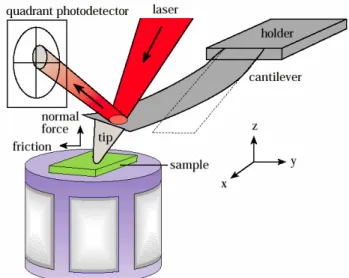
corresponding to a measured displacement. Figure 1 shows a schematic of a common AFM configuration. A thin cantilever (typically between 0.5 and 4μm thick, tens of μm wide by a few hundred μm long) is attached to a fixed holder. The sample under investigation is held on a movable stage. The stage is usually a piezoelectric scanner, designed such that the position of the sample relative to the cantilever can be controlled with sub-nanometer resolution. A laser is directed so as to reflect off the back of the cantilever and onto a quadrant photo-detector. The laser spot moves slightly as the cantilever is deflected, so the angle of deflection of the cantilever is a function of the voltage difference between the top and bottom halves of the photo-detector. Similarly, the difference between the intensity of the light received on each side is related to the torsion of the cantilever.
Figure 1: Schematic of atomic force microscope system including cantilever probe, displacement scanner and laser/quadrant photo-detector. (from R. Carpick, Nanomechanics course notes,
Univ. Wisconsin-Madison.)
In order to find the force that the probe tip exerts on the sample, the stiffness relating deflections at the end of the cantilever to loads at the tip of the AFM probe must be identified. AFM calibration is a difficult inverse problem because only a few characteristics of the probes can be easily measured.
A variety of calibration procedures have been proposed. Tortonese and Kirk attempted to measure the spring constant of AFM probes by using them to deflect a lever of known stiffness [7]. The total stiffness of the two-lever system can then be measured, and from it the stiffness of the AFM probe determined. One advantage of this method is that it does not require that the AFM probe have a pre-defined shape, and it may allow for SI traceable calibration [8]. However, it is not the method of choice in many cases because it requires a “rather laborious process” [9] in which the AFM probe tip is placed precisely on the end of the reference cantilever and because stick slip motion between the AFM probe and the reference cantilever could invalidate the calibration [9]. Furthermore, the accuracy may be limited due to inherent uncertainty in the stiffness of the reference cantilever, which itself must be calibrated.
The most widely applied calibration procedures are based on the dynamic properties of the AFM probe. Cleveland recognized that the probe stiffness could be determined by measuring the in-plane dimensions of the cantilever, assuming that the density of the probe was some nominal value and then measuring the resonance frequency and using it to determine the stiffness of the cantilever [10]. Uncertainty in the density of the cantilever limits the effectiveness of that method, especially for silicon nitride cantilevers where the exact composition realized by the chemical vapor deposition process is not necessarily known. McFarland et al. extended that method to estimate all of the dimensions of tip-less cantilevers [11], but their method still required a priori knowledge of all of the material properties. Cleveland proposed another alternative that determines the stiffness and density of the AFM probe by measuring both the first resonance frequency and the shift in the resonance frequency when beads of known mass are attached to the tip [10, 12]. Uncertainty in the size and density of the beads limits the accuracy of the technique, and there is a risk of damaging the AFM probe, but this method has proved quite effective. However, in recent years, the most commonly used calibration methods seem to be the
method of Sader [13] and the Thermal method of Hutter & Bechhoefer [14], which are both nondestructive and relatively simple to implement. The former derives an analytical model for the interaction of the cantilever with the surrounding fluid (typically air) and uses this to solve for the unknown density per unit area and stiffness of the cantilever from measurements of its resonance frequency and Q-factor in the fluid. The latter utilizes the equipartition theorem to find the cantilever’s spring constant from the magnitude of its mean-square thermal vibration in air or in vacuum. These methods have recently been combined [15] to allow one to find both the stiffness of the AFM probe and the AFM’s displacement sensitivity without bringing the probe in contact with a surface. The displacement sensitivity is usually determined by pressing the tip on a hard surface, which may damage delicate tips, such as carbon-nanotube or functionalized tips.
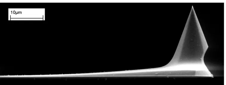
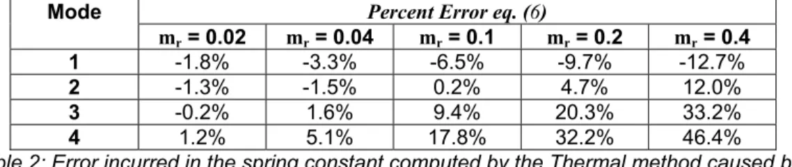
One important limitation of all available dynamic calibration methods is that they neglect the mass of the probe tip, which can be very significant for some probes [16, 17]. Figures 2 and 3 show SEM images of an AFM probe that was studied in a previous work [16, 17], where the authors investigated the effect of neglecting the probe tip on the Sader calibration method. That work showed that the error incurred due to neglecting the tip was only a few percent if the first mode was used in the calibration, while errors of 20% or more could be obtained if the second or higher modes were used to calibrate the probe. The error was generally on the order of the ratio of the tip’s mass to the beam’s mass. This work evaluates the error incurred by neglecting the mass of the AFM tip using the Thermal method of Hutter and Bechhoefer [14]. The tip is found to have a very different effect on the Thermal method than that which was found for the Sader method, revealing cases in which one method or the other would be expected to be more accurate. Also, a corrected calibration procedure is developed that can be used to avoid errors when the tip’s mass can be estimated.
Figure 2: SEM image of an AFM Cantilever from the batch studied in [17] and referenced in this work. The shorter cantilever in the background is also mounted on the same chip.
Figure 3: SEM image showing the geometry of the tip of the probe above. The tip appears to be relatively massive in relation to the beam.
2. Effect of Tip Mass on Thermal Calibration Method
The Thermal method was originally proposed by Hutter and Bechhoefer [14], although there were various corrections and enhancements that others presented subsequently that are important to implement the method correctly [18-20], as clearly outlined by Cook et al. [21]. The method is derived using the equipartition theorem,
which states that the mean kinetic or potential energy of each mode of a cantilever when excited by only thermal noise is equal to (1/2)kBT, where kB = 1.380e-23 J/Kis Boltzman’s constant and T is the absolute temperature. This section modifies the derivation in the works cited above to account for the change in the eigenfunctions of the AFM probe that a tip-mass causes.
Following the derivation in [21], one obtains the following expression for the static stiffness of the
cantilever in terms of Boltzman’s constant, the absolute temperature, the eigenfunction at the tip of the cantilever
ψ(1), the stiffness coefficient knn given in eq. (2), the factor χ given in eq. (3), and the mean square displacement amplitude of the tip
( )
d
c* 2 , where the * denotes that the tip displacement is measured using the optical-lever technique.( )
( )
2 2 2 *1
3
B n s nn n ck T
k
k
d
ψ
χ
⎛
⎞
⎜
⎟
=
⎜
⎟
⎝
⎠
(1)( )
2 1 2 2 0 nn nd
k
x
dx
dx
ψ
⎛
⎞
= ⎜
⎟
⎝
⎠
∫
(2)In order to determine dc*, one must first find the constant of proportionality, S, between the displacement of the tip of the cantilever and the photo-detector voltage. This is usually done by quasi-statically pressing the tip into a rigid surface and measuring the photo-detector voltage as the tip is displaced a known amount. Then, S = ∆V/∆d [21]. The photo-detector actually measures the rotation of the beam at the point at which the laser spot
illuminates it, so this factor is related to the amount that the beam rotates when statically displaced. On the other hand, thermal calibration is performed when the cantilever is vibrating freely. The factor χ was introduced to account for this discrepancy by relating the rotation at the tip of the beam in its statically deformed shape to that in its freely vibrating shape. The required correction is the ratio of the rotation of the beam tip during a static
deflection to that of the free-cantilever vibrating in its nth-mode [21].
( )
( )
( )
1
1 /
1
static n n nu
χ
ψ
ψ
′
=
′
(3),where ustatic(x) = (3x2-x3)/2 is the static displacement of the beam in terms of the non-dimensional position x, scaled such that ustatic(1) = 1. This expression must be modified if the laser spot is large or not at the very tip of the cantilever, as described by Walters et al. [19]. An online calculator is available to compute the correction for a tip-less cantilever at http://bioforce.centech.de. Assuming the laser spot is small and at the tip of the beam, one obtains the following calibration equation.
( )
( )
2 2 *ˆ 1
4
3
n B s nn ck T
k
k
d
ψ
⎛
′
⎞
⎜
⎟
=
⎜
⎟
⎝
⎠
(4)Note that the leading terms in eq. (4) are not shown in most works; these terms are usually lumped to give the following for a tip-less beam with the laser spot at the end of the beam (χ = 1.09) and when the response of only the first mode contributes to
( )
d
c* 2 .( )
* 20.817
B s ck T
k
d
=
(5)On the other hand, if the tip is not negligible, the values traditionally used for χn, ψn(x), and knn, based on a tip-less probe are not appropriate, and calibration based on them introduces error.
2.1. Corrected Thermal Tune Method
The Ritz method was used to find the mode functions of an Euler-Bernoulli beam with a rigid tip, as described in the text by Ginsberg [22], and elaborated for the case of the AFM by the authors in [16]. The
problem was nondimensionalized by dividing through by the beam’s mass, so the important parameter is the ratio, mr, of the tip mass to the beam mass. The rotatory inertia of an AFM probe tip was neglected because it is usually much less important than the mass ratio for the first few modes. Figure 4 shows the mode shapes of a cantilever beam with a tip-mass for various tip mass ratios, spanning the range of those important for AFM.
-2 -1 0 1 2 M ode # 2 -2 -1 0 1 2 3 M ode # 3 0 0.2 0.4 0.6 0.8 1 -2 -1 0 1 2 M ode # 4 Position (nd) 0 1 2 3 M ode # 1
Analytical Mode Shapes for Various Tip Mass Ratios m r = 0 mr = 0.02 m r = 0.04 m r = 0.1 mr = 0.2 mr = 0.4 m r = 0.8
Figure 4: Mode shapes of cantilever beam with a tip mass for various mass ratios mr.
As the mass ratio increases, the amplitude of vibration at the end of the beam decreases, until at mr = 0.8 the end of the beam appears to be almost pinned for the 2nd, 3rd and 4th modes. This model was shown to agree
quite well with experimentally measured mode shapes from an AFM probe with a tip in [16, 17]. In that application the mass ratio was computed to be 0.109 based on volume measurements of the tip from SEM images, and the model was verified by observing that the mode shapes of the model with mr = 0.1 agreed well with those measured experimentally.
This model was used to derive a corrected Thermal calibration method. The analytical mode shapes for the beam with a tip were used in eq. (4) to derive the leading constant that should be used in eq. (5) for a probe with a tip. The constants are shown in Table 1 for various tip-mass ratios, and for the first four modes, any of which can typically be used to perform the calibration. All of these constants assume an infinitesimal laser spot positioned exactly on the tip of the beam [19].
Leading Constant eq. (5) Mode mr = 0 mr = 0.02 mr = 0.04 mr = 0.1 mr = 0.2 mr = 0.4 1 0.817 0.833 0.845 0.875 0.905 0.936 2 0.251 0.254 0.255 0.251 0.240 0.224 3 0.0863 0.0865 0.0849 0.0789 0.0717 0.0648 4 0.0441 0.0436 0.0420 0.0374 0.0334 0.0301
Table 1: Leading constant that should be used in eq. (5) to account for probe tip using Thermal method for various tip-beam mass ratios.
The values in the first column are the same as those available in the literature (they can also be found using the online calculator at http://bioforce.centech.de [20, 23]). As the tip mass ratio increases, the constants generally become increasingly different from their tip-less values, so larger errors are incurred. Denoting the χn,
ψn(x), and knn, that account for the tip with hats (^) and comparing eq. (4) in both cases, the error in the calibrated spring constant is given by the following.
( )
( )
2 , ,ˆ
1
(%) 100
100
1
ˆ 1
s s true nn n n s true nn nk
k
k
Error
k
k
ψ
ψ
⎡
⎛
⎞⎛
′
⎞
⎤
−
⎢
⎥
=
=
⎜
⎜
⎟⎜
⎟
⎜
′
⎟
⎟
−
⎢
⎝
⎠
⎝
⎠
⎥
⎣
⎦
(6) The error is purely a function of the mode shapes of the cantilever (knn are related to the mode shapes viaeq. (2)). The method used to scale the eigenfunctions irrelevant, because the combination ψ’n(x) and knn, cancels any scale factors. It is interesting to note that the error incurred in the Thermal method depends not only on the integral term knn, but also on the slope of the cantilever at the point where the laser reflects from the beam ψ’n(1). In contrast, the authors’ previous work [16, 17] showed that the error incurred when using the method of Sader depended only on the integral terms knn and mnn. Hence, one would expect that the Thermal method may be more sensitive to the tip mass than the Sader method.
The mode functions shown in Figure 4 were used to compute the error in the spring constant for each tip mass ratio using eq. (6). The results are shown in Table 2. The error incurred by neglecting the tip mass is generally on the same order as the tip-mass ratio, which is surprising because one would expect the ratio of the effective masses to be the governing parameter, whereas the mass ratio relates the actual tip mass to the total mass of the beam. The error is also heavily dependent on the mode that is used, with the 3rd mode being least
sensitive at mr=0.02, while the second is less sensitive at mr=0.1. This is quite a different result than that obtained for the Sader method, where the first mode was found to be affected only very slightly by the tip mass for all mass ratios, while the higher modes were much more sensitive. The authors previously studied a set of low spring constant Mikromasch CSC38 AFM probes that had mr= 0.1 [17]. These results show that the error for those probes is between -6.5% and -17.8% for the Thermal method depending on which mode is used in the calibration. The error in the Sader method with mr = 0.1 was 0.2%, 8%, 10% and 10% for the first through fourth modes respectively.
Percent Error eq. (6)
Mode mr = 0.02 mr = 0.04 mr = 0.1 mr = 0.2 mr = 0.4 1 -1.8% -3.3% -6.5% -9.7% -12.7% 2 -1.3% -1.5% 0.2% 4.7% 12.0% 3 -0.2% 1.6% 9.4% 20.3% 33.2% 4 1.2% 5.1% 17.8% 32.2% 46.4%
Table 2: Error incurred in the spring constant computed by the Thermal method caused by neglecting the tip-mass.
2.2. Published Comparisons
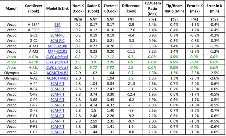
The authors are in the process of validating these results experimentally. In the meantime, there are a few results in the literature that may support these findings. Many studies of AFM calibration have used tip-less cantilevers [24], thus circumventing this issue, but there are a few that have employed commercial cantilevers with tips [9, 21]. For example, Cook et al. compared the Sader and Thermal methods for various cantilevers. Table 3 shows some of their results in the leading columns, including the nominal stiffness of each probe, those estimated using the Sader and Thermal methods, and the percent difference between the two.
The authors computed the volume of the tip for each of the probes listed, using the manufacturer’s specified tip angles for the Veeco probes, and the SEM images in the product literature for the Olympus probes. The beam volume was computed using the manufacturer’s nominal thickness. The ratio of the two was found and is reported in the table. The volume ratio is equivalent to the mass ratio if the density is uniform. The
manufacturer reported a range for the tip height for most of these probes, so those values were used to estimate bounds on the tip/beam mass ratios, both of which are shown in Table 3. However, these should not necessarily be interpreted as complete bounds on the ratio, because our experience has shown that the actual tip geometry can vary significantly from the manufacturer’s specifications.
Manuf. Cantilever
(Cook) Model & Link
Nom K (Cook) Sader K (Cook) Thermal K (Cook) Difference (Cook) Tip/Beam Ratio (Max) Tip/Beam Ratio (Min) Error in K (max) Error in K (min) N/m N/m N/m (%) (%) (%) (%) (%)
Vecco A‐ESP4 ESP 0.2 0.17 0.17 ‐2.9 1.4% 0.4% ‐1.3% ‐0.4%
Vecco A‐ESP5 ESP 0.2 0.12 0.10 ‐17.6 1.4% 0.4% ‐1.2% ‐0.4%
Vecco G‐C1 SCM‐PIC 0.2 0.19 0.19 ‐4.4 0.9% 0.3% ‐0.8% ‐0.2%
Vecco G‐C2 SCM‐PIC 0.2 0.21 0.21 ‐3.3 0.9% 0.3% ‐0.8% ‐0.2%
Vecco A‐M1 MPP‐32100 0.1 0.22 0.20 ‐9 3.3% 1.4% ‐2.8% ‐1.2%
Vecco A‐M2 MPP‐32101 0.1 0.23 0.20 ‐11.1 3.3% 1.4% ‐2.8% ‐1.2%
Vecco A‐F1a CLFC (tipless) 0.2 0.12 0.12 0.7 0.0% 0.0% 0.0% 0.0%
Vecco A‐F1b CLFC (tipless) 1.3 0.9 0.96 6.9 0.0% 0.0% 0.0% 0.0% Vecco A‐F1c CLFC (tipless) 10.4 6.72 6.82 1.5 0.0% 0.0% 0.0% 0.0% Olympus A‐A1 AC240TM‐B2 2.0 1.02 1.04 0.7 1.3% 1.3% ‐2.5% ‐2.5% Olympus A‐A2 AC240TM‐B2 2.0 1 1.04 3.9 1.3% 1.3% ‐2.6% ‐2.6% Vecco A‐P4 SCM‐PIT 2.8 1.04 0.84 ‐21.3 2.3% 0.7% ‐2.0% ‐0.6% Vecco B‐P4 SCM‐PIT 2.8 2.17 2.47 13 2.2% 0.7% ‐2.0% ‐0.6% Vecco C‐P8 SCM‐PIT 2.8 3.74 3.30 ‐12.4 1.9% 0.6% ‐1.7% ‐0.5% Vecco C‐P9 SCM‐PIT 2.8 3.68 3.45 ‐6.2 1.9% 0.6% ‐1.7% ‐0.5% Vecco C‐P7 SCM‐PIT 2.8 4.14 4.32 4.6 2.0% 0.6% ‐1.8% ‐0.5% Vecco D‐P3 SCM‐PIT 2.8 1.5 1.40 ‐68 2.5% 0.7% ‐2.2% ‐0.7% Vecco E‐P1 SCM‐PIT 2.8 2.48 2.26 ‐9.2 2.1% 0.6% ‐1.9% ‐0.6% Vecco E‐P2 SCM‐PIT 2.8 2.59 2.35 ‐9.7 2.0% 0.6% ‐1.8% ‐0.5% Vecco F‐P1 SCM‐PIT 2.8 1.39 1.41 1.9 2.2% 0.7% ‐2.0% ‐0.6% Vecco F‐P2 SCM‐PIT 2.8 1.44 1.31 ‐8.8 2.1% 0.6% ‐1.9% ‐0.6%
Table 3: Comparison of Spring Constants estimated by Sader and Thermal Methods from Cook et al. [21]. The ratio of the tip volume to beam volume was computed and is also shown, along
with the error that would be incurred in K based on the analysis in this paper.
The volume (mass) ratios were used to estimate the error in the spring constant that would have been obtained using the tip-less Thermal method, and the maximum and minimum errors are shown. Cook’s results show that Thermal method tended to underestimate the spring constant for most of the cantilevers. This would agree with the results presented here, which show that the tip mass causes the Thermal method to underestimate the true stiffness, whereas the Sader method is almost insensitive to the tip mass if the first mode was used in the calibration. Unfortunately, all of the probes in the table have very small volume ratios, and there is considerable scatter so this correspondence is far from conclusive.
3. Conclusions
Stiffness calibration is important in most applications of Atomic Force Microscopy. Available dynamic calibration methods neglect the effect of the probe tip on the calibration, even though its effective mass can be
considerable, especially for the thinnest, softest cantilevers used for some of the most sensitive force measurements. The overall uncertainty in AFM calibration is usually estimated to be 10-20%, based on
repeatability and comparisons among methods [25]. This work shows that the error incurred by neglecting the tip mass can be an important contributor to this uncertainty for tip mass ratios as small as mr = 0.1, so it certainly should be considered when calibrating with the Thermal method. For the thinnest, softest cantilevers the error can be quite significant, especially if the higher modes are used in the calibration. The error for two such probes used by the authors with mr = 0.1 and mr = 0.2 is estimated to be -6.5% and -9.7% respectively if the first mode is used, but can be more than 30% if the fourth mode is used. The results also show that the neglected tip mass always causes the Thermal method to underestimate the probe stiffness if the first mode is used in the calibration, although it may be overestimated or nearly exact if other modes are used. One can use this feature to their advantage, using the corrected procedure presented here for multiple modes simultaneously to obtain the most accurate calibration possible. This might also provide an estimate of the uncertainty in the spring constant and a much needed verification that the calibration is accurate.
References
[1] R. Garcia and R. Perez, "Dynamic atomic force microscopy methods," Surface Science Reports, vol. 47, pp. 197-301, 2002.
[2] B. Cappella, H. J. Butt, and M. Kappl, "Force measurements with the atomic force microscope: Technique, interpretation and applications," Surface Science Reports, vol. 59, pp. 1-152, 2005.
[3] G. U. Lee, D. A. Kidwell, and R. J. Colton, "Sensing discrete streptavidin-biotin interactions with atomic force microscopy," Langmuir, vol. 10, pp. 354-357, 1994.
[4] E. L. Florin, V. T. Moy, and H. E. Gaub, "Adhesion forces between individual ligand-receptor pairs," Science, vol. 264, pp. 415-17, 1994.
[5] V. T. Moy, E.-L. Florin, and H. E. Gaub, "Intermolecular forces and energies between ligands and receptors," Science, vol. 266, pp. 257-259, 1994.
[6] R. W. Carpick and M. Salmeron, "Scratching the surface: fundamental investigations of tribology with atomic force microscopy," Chemical Reviews, vol. 97, p. 1163, 1997.
[7] M. Tortonese and M. Kirk, "Characterization of application specific probes for SPMs." vol. 3009 San Jose, CA, USA: SPIE-Int. Soc. Opt. Eng, 1997, pp. 53-60.
[8] G. A. Shaw, J. Kramar, and J. Pratt, "SI-traceable spring constant calibration of microfabricated cantilevers for small force measurement," Experimental Mechanics, vol. 47, pp. 143-51, 2007.
[9] N. A. Burnham, X. Chen, C. S. Hodges, G. A. Matei, E. J. Thoreson, C. J. Roberts, M. C. Davies, and S. J. B. Tendler, "Comparison of calibration methods for atomic-force microscopy cantilevers,"
Nanotechnology, vol. 14, pp. 1-6, 2003.
[10] J. P. Cleveland, S. Manne, D. Bocek, and P. K. Hansma, "A nondestructive method for determining the spring constant of cantilevers for scanning force microscopy," Review of Scientific Instruments, vol. 64, pp. 403-5, 1993.
[11] A. W. McFarland, M. A. Poggi, L. A. Bottomley, and J. S. Colton, "Characterization of microcantilevers solely by frequency response acquisition," Journal of Micromechanics and Microengineering, vol. 15, pp. 785-91, 2005.
[12] T. J. Senden and W. A. Ducker, "Experimental determination of spring constants in atomic force microscopy," Langmuir, vol. 10, pp. 1003-1004, 1994.
[13] J. E. Sader, J. W. M. Chon, and P. Mulvaney, "Calibration of rectangular atomic force microscope cantilevers," Review of Scientific Instruments, vol. 70, pp. 3967-9, 1999.
[14] J. L. Hutter and J. Bechhoefer, "Calibration of atomic-force microscope tips," Review of Scientific Instruments, vol. 64, pp. 1868-73, 1993.
[15] M. J. Higgins, R. Proksch, J. E. Sader, M. Polcik, S. M. Endoo, J. P. Cleveland, and S. P. Jarvis, "Noninvasive determination of optical lever sensitivity in atomic force microscopy," Review of Scientific Instruments, vol. 77, pp. 13701-1, 2006.
[16] M. S. Allen, H. Sumali, and E. B. Locke, "Experimental/Analytical Evaluation of the Effect of Tip Mass on Atomic Force Microscope Calibration," in 26th International Modal Analysis Conference (IMAC XXVI) Orlando, Florida, 2008.
[17] M. S. Allen, H. Sumali, and P. C. Penegor, "Experimental/Analytical Evaluation of the Effect of Tip Mass on Atomic Force Microscope Calibration," ASME Journal of Dynamic Systems, Measurement and Control, vol. Submitted May 2008, 2008.
[18] H. J. Butt and M. Jaschke, "Calculation of thermal noise in atomic force microscopy," Nanotechnology, vol. 6, p. 1, 1995.
[19] D. A. Walters, J. P. Cleveland, N. H. Thomson, P. K. Hansma, M. A. Wendman, G. Gurley, and V. Elings, "Short cantilevers for atomic force microscopy," Review of Scientific Instruments, vol. 67, p. 3583, 1996. [20] R. Proksch, T. E. Schaffer, J. P. Cleveland, R. C. Callahan, and M. B. Viani, "Finite optical spot size and
position corrections in thermal spring constant calibration," Nanotechnology, vol. 15, pp. 1344-1350, 2004.
[21] S. M. Cook, T. E. Schaffer, K. M. Chynoweth, M. Wigton, R. W. Simmonds, and K. M. Lang, "Practical implementation of dynamic methods for measuring atomic force microscope cantilever spring constants," Nanotechnology, vol. 17, pp. 2135-45, 2006.
[22] J. H. Ginsberg, Mechanical and Structural Vibrations, First ed. New York: John Wiley and Sons, 2001. [23] T. E. Schaffer, "Calculation of thermal noise in an atomic force microscope with a finite optical spot size,"
Nanotechnology, vol. 16, pp. 664-70, 2005.
[24] B. Ohler, "Cantilever spring constant calibration using laser Doppler vibrometry," Review of Scientific Instruments, vol. 78, pp. 63701-1, 2007.
[25] B. Ohler, "Application Note #94: Practical Advice on the Determination of Cantilever Spring Constants," in Veeco Application Notes. vol. http://www.veeco.com/library, 2007.