On the use of Silhouette for cost based clustering

(1)

Università degli Studi di Padova

Department of Ingegneria dell’Informazione

Master Thesis inIngegneria Informatica

On the use of Silhouette for cost based clustering

Supervisor Master Candidate

Dott. Fabio Vandin Marco Sansoni

(2)

(3)

Abstract

Clustering plays a fundamental role in Machine Learning. With clustering we refer to the problem of finding coherent groups in a dataset of elements. There are several algorithms to perform clustering that have been proposed in the literature, considering different costs for the optimization problems they consider. In this thesis we study the problem of cluster-ing when the cost function is the silhouette coefficient, an index traditionally used for the internal validation of the results oof clustering algorithms. In particular, we propose and analyze some heuristic algorithms to identify the clustering maximizing the silhouette value, and compare their results with the results from some widely used clustering algorithms.

(4)

(5)

2.2 Euclidean Distance . . . 4 2.3 Jaccard Distance . . . 5 2.4 Edit Distance . . . 6 2.5 Hamming Distance . . . 6 2.6 Clustering . . . 7 2.7 K-Means . . . 9 2.7.1 K-Means ++ . . . 11 2.8 K-Medoid . . . 13 2.9 Clustering Validation . . . 15 3 Related Work 21 3.1 An Immune Network Algorithm for Optimization . . . 21

3.2 Evolutionary Algorithm for Clustering . . . 22

3.3 Soft-Silhouette . . . 23

4 Goal 25 5 Algorithm for Clustering using Silhouette as cost 27 5.1 Brute Force Approach . . . 27

5.1.1 Description of the Approach . . . 27

5.1.2 Code . . . 28

5.1.3 Complexity and Correctness . . . 29

5.2 Extending K-Means . . . 35

5.2.2 Pseudo Code . . . 35

(6)

5.2.5 Improvement . . . 45

5.3 PAMSILHOUETTE . . . 48

5.3.2 Initial Seeding Technique for Partitioning Around Medoid Algo-rithm: BUILD . . . 49

5.3.3 Pseudo Code . . . 52

5.3.4 Choice of Parameters . . . 54

5.4 ExtendePAM . . . 58

5.4.2 Pseudo Code . . . 58

5.5 Improved version of extendePAM, extendePAMv2 . . . 63

6 Experimental evaluation 67 6.1 Dataset . . . 67

6.2 Implementation . . . 71

6.3 Comparison of commonly used Clustering Algorithms . . . 72

6.4 Brute Force Approach . . . 75

6.5 Extende K-Means and Improved version . . . 77

6.5.1 Reduced Dataset . . . 77 6.5.2 Complete Dataset . . . 80 6.6 PAMSILHOUETTE . . . 83 6.6.1 Reduced Dataset . . . 84 6.6.2 Complete Dataset . . . 84 6.7 extendePAM . . . 85 6.7.1 Reduced Dataset . . . 85 6.7.2 Complete Dataset . . . 87 7 Conclusion 91 References 94

(7)

Listing of figures

2.1 Jaccard Distance is5/8. Taken from [1]. . . 5

2.2 Dendogram representing Hierarchical Clustering. Taken from [1]. . . 9

2.3 Bad initial seeding. Taken from [2]. . . 11

2.4 K-medoids versus K-means. Taken from [3]. . . 14

2.5 Elbow Method. Taken from [4]. . . 17

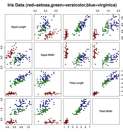
6.1 Iris Dataset. Each plot shows distribution of the sample filtering for only 2 features. Taken from [5]. . . 68

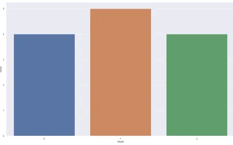
6.2 Reduced Iris dataset. 1,2 and 3 is used to labelling three classes of iris . . . . 69

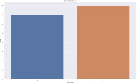
6.3 Reduced Breast Cancer Wisconsin Data Set. 2 and 4 is used to labelling two kinds of cancer, benign or malignant . . . 70

6.4 Reduced banknote authentication dataset. 0 and 1 is used to labelling two different classes of banknote . . . 71

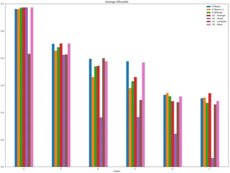
6.5 Histogram of Average Silhouette value on Iris Dataset from most famous clustering algorithm . . . 73

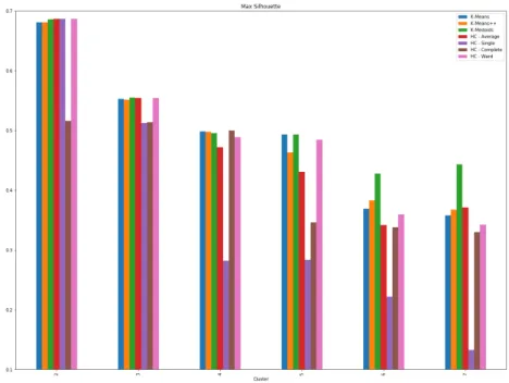
6.6 Histogram of maximum Silhouette value on Iris Dataset from most famous clustering algorithm . . . 74

6.7 Histogram of Silhouette value and time required in seconds for execution ofbruteF orceon Reduced Iris Dataset . . . 76

6.8 Histogram of Silhouette value and time required in seconds for execution ofbruteF orceon Reduced Breast Cancer Dataset . . . 78

6.9 Histogram of Silhouette value and time required in seconds for execution ofbruteF orceon Reduced Banknote Dataset . . . 79

6.10 Histogram of increment of Silhouette value obtained forextendeKM eans andextendeKM eansv2algorithm related tok −M eansresults. Line refers to time required in seconds for termination of the algorithm. Algo-rithms are applied on Iris Dataset . . . 81

6.11 Histogram of increment of Silhouette value obtained forextendeKM eans andextendeKM eansv2algorithm related tok −M eansresults. Line refers to time required in seconds for termination of the algorithm. Algo-rithms are applied on Breast Cancer Dataset . . . 82

6.12 Histogram of increment of Silhouette value obtained forextendeKM eans andextendeKM eansv2algorithm related tok −M eansresults. Line refers to time required in seconds for termination of the algorithm. Algo-rithms are applied on Breast Cancer Dataset . . . 83

(8)

7.1 Comparison of the maximum value of Silhouette achieved from all the al-gorithm involved into this thesis on Iris Dataset . . . 91 7.2 Comparison of the maximum value of Silhouette achieved from all the

al-gorithm involved into this thesis on Breast Cancer Dataset . . . 92 7.3 Comparison of the maximum value of Silhouette achieved from all the

(9)

Listing of tables

6.1 Comparison of Average Silhouette value on Iris Dataset from most famous

clustering algorithm . . . 73 6.2 Comparison of maximum Silhouette value on Iris Dataset from most

fa-mous clustering algorithm . . . 74 6.3 Silhouette Results performed from BruteForce algorithm on reduced

ver-sion of Dataset . . . 76 6.4 Evaluation of time required and number of k-subsets for each number of

cluster performed on Reduced version of Iris Dataset . . . 77 6.5 Evaluation of silhouette value obtained after execution ofextendeKmeans

and its improved version on reduced Iris Dataset . . . 77 6.6 Evaluation of silhouette value obtained after execution ofextendeKmeans

and its improved version on reduced Breast Cancer Dataset . . . 79 6.7 Evaluation of silhouette value obtained after execution of extendeKMeans

and its improved version on reduced Banknote Dataset . . . 80 6.8 Results of silhouette and time required after execution ofKM eans,extendeKM eans

andextendeKM eansv2on Iris Dataset . . . 80 6.9 Results of silhouette and time required after execution ofKM eans,extendeKM eans

andextendeKM eansv2on Breast Cancer Dataset . . . 82 6.10 Results of silhouette and time required after execution ofKM eans,extendeKM eans

andextendeKM eansv2on Banknote Dataset . . . 83 6.11 Silhouette value obtained after application ofP AM SILHOU ET T E

al-gorithm on reduced version of Dataset . . . 84 6.12 Silhouette value obtained after application ofP AM SILHOU ET T E

al-gorithm on complete version of Dataset . . . 85 6.13 Time in seconds required for application ofP AM SILHOU ET T E

algo-rithm on complete version of Dataset . . . 85 6.14 Evaluation of Silhouette value obtained after execution ofextendeP AM

and its improved version on reduced Iris Dataset . . . 86 6.15 Evaluation of Silhouette value obtained after execution ofextendeP AM

and its improved version on reduced Breast Cancer Dataset . . . 87 6.16 Evaluation of Silhouette value obtained after execution ofextendeP AM

and its improved version on reduced Banknote Dataset . . . 87 6.17 Results of silhouette and time in seconds required after execution ofP AM,

(10)

6.18 Results of silhouette and time in seconds required after execution ofP AM,

extendeP AM andextendeP AM v2on Breast Cancer Dataset . . . 88 6.19 Results of silhouette and time in seconds required after execution ofP AM,

(11)

1

Introduction

One of the biggest challenges in Machine learning and Data Mining is the detection, classi-fication and validation of cluster. Although there is no single consensus on the definition of a cluster, the clustering procedure can be characterised as the organisation of data into a finite set of categories by abstracting their underlying structure, grouping object in a single partition to describe data according to a similarities or relationship among its object. Clus-tering could ﬁnd an usage for several applications, such as identification of customer proﬁle, anomaly detection and market segmentation. A difficulty common to many clustering tech-niques is that they may need to providea −priorinumber ofk different clusters in the database. This constraint makes algorithms less powerful and efficient, because they require a domain knowledge for tuning the parameter that fits the data. The lack of a common def-inition of cluster makes it a widely studied subject, with the presence in literature of many different approaches to the clustering problem. Each technique is characterised by a different metric to allocate the data into relative clusters, each one producing different results. Even the application of the same method may generate, as output, different clusters for each ex-ecution of the algorithm. This poses difficulties to users, who not only have to select the clustering algorithm best suited for a particular task, but also have to properly tune its pa-rameters. Such choices are related to clustering validation, another widely researched topics in clustering literature. A common approach to evaluate a quality of a cluster is by the usage of internal criteria. These measures provide a metric of clustering inspecting only the intrin-sic information available in the data. Many different criteria have been proposed in literature,

(12)

however the majority of them are based on the idea of computing the ratio of within-cluster scattering (compactness) to between cluster separation[6]. In this thesis it will be presented some new algorithms for the clustering problem. First of all, we provide a brief overview of the background knowledge required for a later analysis of the content available in the the-sis. We highlight the main approach used nowadays for clustering, inspecting some critical aspects for each of them. Furthermore, methods of cluster validation are presented. We refer to them as a tool to evaluate the goodness of a clustering algorithm. Even if it is possible to detect many of them employed into a real scenario, we will focus on the details of a specific statistics, Silhouette. According to its definition we propose some implementations of a clus-tering technique that aims to its maximisation. For the developing of this specific task we will present several approaches, described into chapter 5. Each algorithm is evaluated analysing pro and cons, with an emphasis on the complexity of the algorithm. In chapter 6 we de-scribe all the experimental results obtained on the application of previous algorithms on 3 dataset, with different number of samples and features. We conclude this thesis with a brief discussion regarding the effectiveness of the algorithm presented compared with the most used clustering algorithm.

(13)

2

Background

In the current section we are going to define the basics of clustering, starting with the def-inition of distance between points, to conclude with the main approach of clustering and commonly used measure for validation.

2.1 Point and Distances

Domain of any clustering problem is a set of finite pointsX. Considering the common case of the Euclidean space we define a point asxi ∈ X. Each one has associated a vector of

real values, which components are commonly calledcoordinatesof the represented points. Besides the definition of a point it is necessary to provide a definition of distance, in fact it can be employed to represent a similarity or dissimilarity between points.

Given a set of pointXandx, y ∈ X, a distance measure between them is represented by

d(x, y). It has to produce a number as output and it follows the following axioms: - d(x, y)>0: distance cannot be negative.

- d(x, y) = 0if and only ifx =y: distance is zero if and only if we consider distance from a point to itself.

- d(x, z) > d(x, y) +d(y, z), withz ∈ X: distance measure must follow triangle inequality.

(14)

All the following distance measures need to accomplish the previous property. We pro-vide a short explanation of the main measure distance suitable for an Euclidean Space. It is also relevant to show some other possible distance measure for non Euclidean Space. The following sections mention about the most significant and each of them are suitable for a specific purposes.

2.2 Euclidean Distance

The most known distance measure is the most intuitively and simple approach. We assume

n-dimensional points, represented by a vectorx= [x1, x2, . . . , xn]. Euclidean distance, also

refer asL2-norm, is defined as:

d(x, y) = d([x1, x2, . . . , xn],[y1, y2, . . . , yn]) = v u u tXn i=1 (xi−yi)2 (2.1)

Euclidean distance is computed summing up the square root of difference in each dimension, and finally take the positive square root. It is necessary to show that the requirements for a distance are satisfied. In fact, theL2-norm is always positive, as result of positive square root.

Then,(xi −yi)2is positive if we can get an occurrencexi ̸= yi that force the sum to be

strictly positive. On the other hand, only ifxi =yi∀iproduces a distance equal to 0.

Last axiom requires to deal with some maths for the proof. However, we can notice that it is a well-known property of Euclidean space. It reminds that the length of the third side of a triangle cannot be longer of the sum of the other two sides.

From the definition of theL2-norm, we can define theLr-norm on Euclidean Space,

gener-alizing (2.1) for any constantr. It is defined by:

d(x, y) =d([x1, x2, . . . , xn],[y1, y2, . . . , yn]) = ( n

X

i=1

|xi−yi|r)1/r (2.2)

The caser= 2is the usualL2-norm mentioned above. Another relevant distance measure is whenr= 1, it is calledL1-norm orManhattan Distance. It is a measure of the distance that we get travelling from a point to another following grid lines, as the streets of Manhattan. Another important distance is the limit to infinity of 2.2, whenrapproaches to+∞. It has been calledL_∞-norm. Effectively, it can be computed as maximum value of|xi−yi| ∀i.

(15)

2.3 Jaccard Distance

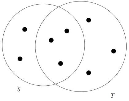
Jaccard Distance is a measure useful when we have to deal with sets. In fact, given two setsx

andy, it is defined by:

d(x, y) = 1− x∩y

x∪y (2.3)

Figure 2.1 shows us a possible instance of the sets, for a better comprehension through visu-alisation. We must now verify the requirements for each distance function.

Figure 2.1:Jaccard Distance is5/8. Taken from [1].

1. Distance is non negative since the intersection of two sets cannot be bigger than the union.

2. d(x, y) = 0if and only ifx=y, because to achieve this result we get an intersection equal to the union of two sets, available only whenx = y. Hence,x∪y=x∩y=

x = y. On the other hand, ifx ̸= y, intersection will always be strictly lower than union.

3. As in the previous section, related to Euclidean distance, proof of triangle inequality requires to deal with a lot of maths. In this thesis the verification will be omitted since it is not relevant for the further developing. In literature there are many proofs of the

(16)

triangle inequality related to Jaccard Distance. For instance, a concise proof can be found in [1].

2.4 Edit Distance

This distance is defined for strings. Given two stringsx=x1x2. . . xnandy=y1y2. . . yn,

an informal definition of this measure is the number of insertions or deletion of single char-acters that will convertxintoy.

For instance, Edit distance betweenx=abcdeandy=acf degis 3, since we need to: 1. Delete b.

2. Insert f after c. 3. Insert g after e.

Another way for the computing of this distance is by the usage ofLongest Common Sub-string(LCS) ofxandy. Once we perform theLCSwe can define the Edit Distance as:

d(x, y) = |x|+|y| −2LCS(x, y) (2.4) Surely no Edit Distance can be negative and only two identical strings can have Edit Distance equal to 0. An idea of the proof of the triangle inequality applied to Edit Distance is to note that for converting a stringsinto a stringtwe need to turn first intou, and then fromuto

t. Hence, number of operations done to turnsintotcannot be less than the sum made to convertsinuand finallyuint.

2.5 Hamming Distance

Given a space of vectors, the Hamming Distance between two vectors is the number of com-ponents in which they differ. It has a wide appliance related to distance between vector of Boolean, composed only by 1’s and 0’s. For the sake of completeness, an example is provided. Givenv1 = 10001andv2 = 10111, counting from the right we get that the second and third occurrence are different. So, the Hamming Distance is 2.

(17)

and it can be equal to 0 only if the vector has the same occurrences, hence the vectors are identical.

As all the others distance measure, Hamming Distance requires more maths, but it should be obvious that it satisfies the triangle inequality. If the distance between a vectorxandz

are ofmcomponents, andzandydiffer inncomponents, it cannot be thatxandydiffer in more thanm+ncomponents.

2.6 Clustering

Recalling the introductory section, a cluster is an organisation of data into a finite set of cate-gories. Since the definition has not a clear and unique value, different clustering algorithms can produce a different division of the points. Hence, we can exploit several approaches of clustering, and we classify algorithms into two main categories, that follow different strate-gies.

1. Hierarchical or agglomerative

Algorithms start with each point into a specific cluster. Then, according to the dis-tance measure employed, two cluster ”close” are fused into a new cluster. This process is iterated over and over until a convergence criteria stops the algorithm.

Criteria that can force the conclusion of the algorithm can be several, for instance if we achieve a number of cluster selected a priori, or if the distance between nearest cluster is over a certain threshold. We can also refuse to merge different clusters that lead to point of a single cluster spread in a large region. Once we define the distance measure in the space and stopping criteriaS, algorithm can be briefly described by Algorithm 2.1.

Into Algorithm 2.1 we describe the common algorithm for all the hierarchical cluster-ing approaches. It is executed untilSforces termination of the algorithm. Examples ofScould be if minimum distance between cluster decreases below a given threshold or if we reach the desired number of clusters. At each iteration of the while loop, two clusters are elected to be merged. Decision of which cluster merge is up to specific linkage criteria of algorithm chosen. Lines 8 and 9 mean that the sample belonging to the cluster to merge are inserted into a new clusterCl, common for both samples, and

previous clusters are deleted.

Finally, we can describe the process done by the algorithm with the tree in Figure 1.2 showing the complete grouping of points.

For the proper functioning of the algorithm is important to define also linkage func-tion between two clusters, in order to detect the elected ones to be merged. According to the choice, result may vary. Linkage are defined according to proximity measure among clusters[7]. Principal approaches are:

(18)

Algorithm 2.1 Hierarchical Clustering

1: Input

2: X dataset

3: S stopping criteria chosen for hierarchical clustering

4: Output

5: C clustering

6: procedure hierarchicalClustering(X,S)

7: whileSdoes not stop the algorithm

8: pick the best two clusterCi, Cjto merge

9: Cl ←Ci∪Cj

10: Ci, Cj ← ∅

11: returnC

• Single Linkage

Proximity between two clusters is the proximity between their two closest ob-jects. Single linkage method controls only nearest neighbours similarity.

• Complete Linkage

Proximity between two clusters is the proximity between their two most distant objects.

• Average Linkage

Proximity between two clusters is the arithmetic mean of all the proximities be-tween the objects of one, on one side, and the objects of the other, on the other side

• Ward Linkage

In order to define this criteria it is required the definition of within cluster vari-ance. According with [8], the within cluster varianceWof a clusterCkis:

W(Ck) =

X

xi∈Ck

d(xi, µk) (2.5)

whereµkis referred to the mean of the clusterCk, also called centroid. Proximity

between two clusters is the within cluster variance of the merged cluster. It aims to minimizes the variance of the cluster being merged.

2. The other class of algorithm involves point assignment.

Points are considered in some order, and each one is assigned to a cluster with best fit. The algorithm is started with the estimation of initial choice of clusters. In this class of algorithms it is fundamental a domain knowledge of the problem since it is

(19)

mandatory the definition ofkclusters where the points will be classified. Points are associated to a specific cluster according to an objective function characteristic of the algorithm. For example, points will be associated to the cluster that minimize theL2

-norm between each point and the centre of the cluster which it is classified, as in the K-means algorithm.

Figure 2.2:Dendogram representing Hierarchical Clustering. Taken from [1].

2.7 K-Means

In this section we shortly explain one of the most famous algorithms of clustering[9]. We initially describe the objective function to be minimized, and then we provide an algorithm that can be really implemented.

They assume Euclidean Space, and the number of clusterkis known in advance.

Given a set of observationx1, x2, . . . , xn, where each observation is a d-dimensional real

vec-tor, k-means clustering aims to partition the observation intok(<=n)setsS ={S1, S2, . . . , Sk}

in order to minimize the within-cluster sum of squares. The purpose is to find:

arg min S k X i=1 X x∈Si ||x−µi| |2 (2.6)

whereµiis the mean of the point inSi. Algorithm 2.2 shows an approach of the min problem

presented into cost function 2.6. Discussion of the algorithm will be made through inspec-tion of the code shown into Algorithm 2.2

K-means represents just an heuristic solution for the minimization of objective function. In fact, a rigorous solution is computationally expensive, so we look for an approximation of

(20)

the optimal result. For a comprehension of the approach we introduce centroid definition. Given a set of d-dimensional pointsW ={w1, w2, . . . , wn}, centroid is expressed as:

c=

n

X

i=1

wi (2.7)

Centroid is a d-dimension point∈/ W, that represents the average value of the points into

W.

Algorithm 2.2 K-Means Algorithm

1: Input

2: X dataset

3: k number of clusters

4: Output

5: C clustering of dataset into k clusters

6: procedure K-Means(X,k)

7: c←kpoints that are likely to be in different clusters

8: make these points centroid of clusters, namedC

9: repeat

10: for allxi ∈X

11: ci ←centroid whichxiis closest

12: addxito clusterCi

13: adjust centroid of clustersCiafter addition ofxi

14: until there are any variations of centroid

15: return C

Algorithm 2.2 requires as inputk, the number of cluster to partition the given dataset. First line generatesc, set ofksamples which we assume as cluster center. Selection is a wide argument that we will discuss later. While we denoted withcthe set of centroid, we indi-cate withC, the clustering of the whole dataset, whereci is the centroid ofCi. Into the

while block, at each iteration we evaluate for each samplexithe centroid closer to it, and we

associate each point to closest cluster. Each iteration of the algorithms also include the re calculation of the centroidc, as expressed into 2.7. Termination criteria of the while block is expressed through stability of the centroid. If there are any variations of centroids among two consecutive iteration, algorithm terminates, otherwise it repeats with a new iteration. A crucial operations into the algorithm is the detection of the initial cluster center. Different approaches are presented for the first center selection, a trivial solution is to pick upkpoints

(21)

randomly on the dataset, but more accurate strategies are available in order to achieve better classification. The most used solution for center selection is reported into section 2.7.1. Key of the algorithm is the repetition of the point assignment. Each point is assigned to the center which minimize its square distance to the cluster, according to:

v u u tXd i=1 d(xi−yi)2 (2.8)

Point assignment strategy for the clustering suffers of the a priori knowledge of the number of final clusterk. The choice of the best value that fit the point is crucial for a good clustering. To overcome this problem, in the literature are present many approaches of clustering valida-tion, that will be presented in section 2.9. Furthermore, K-means suffers the initial choice of the cluster center. For instance, in the situation displayed in Figure 2.3. Here the example (a)

Figure 2.3:Bad initial seeding. Taken from [2].

of a bad initialization that (b) leads to a poor k-Means solution, consisting of clusters with significantly different variances. Instead, a proper seeding leads to example (c). In order to avoid the problem, different techniques are used to reduce probability of such situation. A trivial solution is to execute more times the algorithm, obtaining different results due to the randomness of the initial choice of the center. Hence, we pick up as the best result the clustering that mostly shows off.

2.7.1 K-Means ++

As explained before,K −M eansalgorithm begins withkarbitrary centers, typically cho-sen uniformly at random from the data point. Each point is then assigned to the nearest

(22)

center, referring to 2.8. At each iteration each center is recomputed as the centroid of all points belonging to it. In this scenario, David Arthur and Sergei Vassilvitskii proposedK− M eans+ +in 2007[10]. It is focused on the appliance ofa−priorialgorithm focused only into center selection, in order to substantially reduce the probability of the situation occurred in Figure 2.3. It produces centroids used as initial seeding ofK−M eans. Given a setX ={x1, x2, . . . , xn}, we want to detectkinitial centers, namelyC ={c1, c2, . . . , ck}.

In particular, letD(x)denote the shortest distance from a data point to the closest center. Finally, algorithm is defined into Algorithm 2.3.

Algorithm 2.3 K-Means ++

1: Input

2: X dataset

3: k number of clusters

4: Output

5: c k initial point belonging to dataset used for first center into K-Means

6: procedure K-Means ++(X,k)

7: c1 ←chosen uniformly at random fromX

8: while|c|< k

9: Take new centerci, choosing fromx∈X−Cwith probability

D(x)2

∑

x∈XD(x)

2

10: returnc

Algorithm 2.3 is used to center selection, for this reason the number of clusters is a required parameter. Into the algorithm we indicate withcset of centers. First centerc1is chosen at

random from dataset, all the otherciare chosen according to a probability measure. At the

end of while block,ccontains exactlykpoints, used later for first centers intoK−M eans

algorithm.

We can notice thatK−M eans+ +is a probabilistic algorithm, it means that the output can differ at each execution. As shown in the Algorithm 2.3, the probability of a point to be chosen as a center is:

D(x)2

P

x∈XD(x)

2 (2.9)

Recalling thatD(x)is the distance between a pointxand its closest center inc, the algorithm highlights that the farthest point are chosen as centers with more probability. This seeding method yields considerable improvement in the final error ofk −M eans. Although the

(23)

initial selection in the algorithm takes extra time,k−M eansconverges faster with this initial seeding, lowering the computation time. Thek−means+ +approach has been applied since its initial proposal for center selection.

2.8 K-Medoid

K −M edoidsclustering is an approach that aims to minimize a given cost function[11]. Rather than using conventional centroid, it uses medoids to represent the clusters.

Given a set of pointsX ={x1, x2, . . . , xn}, a medoids, namedxmedoidis:

xmedoid= arg min yin{x1,x2,...,xm}

n

X

i=1

d(y, xi) (2.10)

Here we represent withd(x, y)the dissimilarity function between points. It usually refers at the distanceL2among points. Unlike centroids that usually do not belong to dataset, a

medoid is always a member of the data set. It represents the most centrally located item of the data set. The purpose is to determine the best clusteringCwhich minimizes cost function expressed into 2.11. Each clusteringCi contains a pointci ∈ Ci which represents a central

sample of the cluster.

C = arg min C k X j=1 X i∈Cj d(xi, cj) (2.11)

As for the exact solution of cost function defined into 2.6, even the computation of best clusteringCminimizing 2.11 is a NP-Hard problem. An heuristic solution is presented into

P artitionaroundM edoids(PAM) algorithm.P AMuses a greedy search which may not find the optimum solution, but it is faster than exhaustive search. Given in input the set of points X = {x1, x2, . . . , xn}and the number of clusterk, algorithm can be found into

(24)

Figure 2.4:K-medoids versus K-means. Taken from [3].

Algorithm 2.4 Partition Around Medoid

1: Input 2: X dataset 3: k number of clusters 4: Output 5: C clustering 6: procedure PAM(X,k)

7: selectkof thendata points as the medoidsM

8: associate each data point to the closest medoid

9: while cost of the configuration decreases

10: for allm ∈M

11: for allo /∈M

12: swapmando

13: associate each data point to the closest medoid

14: recompute the cost

15: if total cost increased in the previous step

16: undo the swap

return clustering

P artitioningaroundM edoidis described into Algorithm 2.4. Ask −M eans, it re-quires datasetX, and number of clusters as input of the algorithm. Initially it selectskpoints as medoid, each point intoM has to belong to the dataset. All the other samples are associ-ated to the closest medoid. For each configuration of the setM, cost is the sum of distance from each sample to the closest medoid. Core of the algorithm is the continue swap among a pointm∈Mando /∈M. At each iteration is performed a change amongmando, defin-ing a new sets of medoid. If the new cost function associated to the set of medoids increases, swap is undone. If no swap achieves a reduction of the cost, algorithm concludes reporting

(25)

final clustering, ones with smallest cost function.

These algorithms suffer of the same issues ofk−M eansalgorithm, since they are heuristic solutions, they cannot achieve certainly an exact solution, but an approximate result. There are several different strategies for picking up the initial medoid during initialization phase of the algorithm. As fork−M eans, a simple solution involves selection of medoid uniformly at random from the data point. Most sophisticated approaches can be found in literature to achieve the best solutions at the first executions.

As well ask−M eansit requires as input the number of clusterk. Figure 2.4 highlights a dataset whichP AMalgorithm performs better thank−M eans, subdividing samples into the obvious cluster structure of data set. The image 1a-1f presents a typical example of the k-means convergence to a local minimum. In this example, k-medoids algorithm, showed into images 2a - 2h, with the same initial seeding of k-means converges to the obvious cluster structure.

K-medoids method is more robust than k-means in presence of noise and outliers because a medoids is less influenced by outliers or other extreme values[12].

2.9 Clustering Validation

Since there is not a unique definition of clusters, and some different strategies are proposed, we need to identify a score to classify the results provided from algorithms. In order to over-come this issue a lot of strategies have been produced.

Generally, clustering validation statistics can be categorized into 3 classes: 1. Internal Cluster Validation

It uses internal information of the clustering process to evaluate the goodness of a clustering structure without reference to external information. It can be used for esti-mating the number of clusters and the appropriate clustering algorithm without any external data.

2. External Cluster Validation

It consists in comparing the results of a cluster analysis to an externally known result, such as externally provided class labels. It measures the extent to which cluster labels match externally supplied class labels. Since we know the “true” cluster number in advance, this approach is mainly used for selecting the right clustering algorithm for a specific data set.

(26)

3. Relative Cluster Validation

It evaluates the clustering structure by varying different parameters for the same al-gorithm, such as the number of clustersk. It is generally used for determining the optimal number of clusters.

In this section we will focus on exploiting the intrinsic structure of the data, discussing about internal cluster validation. Here, we present some metrics available in literature. Elbow Method

The Elbow Method [13] looks at the percentage of variance explained as a function of the number of clusters: one should choose a number of clusters so that adding another cluster does not give much better modelling of the data. More precisely, if one plots the percentage of variance explained by the clusters against the number of clusters, the first clusters will add much information (explain a lot of variance), but at some point the marginal gain will drop, giving an angle in the graph. The number of clusters is chosen at this point, hence the ”elbow criterion”. This ”elbow” cannot always be unambiguously identified.

In Figure 2.5 we indicate with a red circle the elbow of the plot. According to this method, the proper number of cluster for such algorithm is 4.

This is one of the most naive approaches. Other similar approaches are available inspecting the average diameter of the cluster instead of the variance. However, a common aspect is identifying k according to the ”elbow” of the plot. The main issue of this approach, as several other techniques of cluster validation, is the fact that it is mandatory to perform clustering with all the possible value ofk, in order to build the graph.

Dunn Index

Dunn Index is a metrics used to evaluate clustering algorithm. It was introduced by J.C. Dunn in 1974[14] [15]. The aims are to identify sets of clusters that are compact, with a small variance between members of the cluster. For a given assignment of cluster, high value of Dunn index means better clustering of data. One of the drawbacks is the computational cost required for the computation of the index.

As a requirement for comprehension of Dunn Index we provide a digression on the size or di-ameter of a cluster. There are different approaches, as the mean distance between two point in a cluster, but for this statistic we consider the farthest two points inside a cluster.

(27)

Figure 2.5:Elbow Method. Taken from [4].

vector belonging into the same clusterCi. The diameter of the cluster is:

∆i = max

x,y∈Ci

d(x, y) (2.12)

Besides the definition of the diameter of the cluster, we require a measure of inter cluster distance metric. Hence, we define:

δ(Ci, Cj) = min x∈Ci,y∈Cj

d(x, y) (2.13)

While distance intra cluster is computed referring to the farthest two points, we consider nearest points for the inter cluster measure. We can finally provide a definition of the Dunn statistic. If we getkcluster, Dunn Index for the set is defined as:

DIk=

min1≤i≤j≤kδ(Ci, Cj)

max1≤i≤k∆i

(2.14) This formulation has a peculiar problem, in that if one of the clusters is badly behaved, where the others are tightly packed, since the denominator contains a ’max’ term instead of an av-erage term, the Dunn Index for that set of clusters will be uncharacteristically low.

(28)

Silhouette Coefficient

Silhouette coefficient has been introduced for the first time by Peter J. Rousseeuw in 1987 [16].

It refers to a method of interpretation and validation of consistency within clusters of data. The silhouette value is measured of how similar an object is to its own cluster (cohesion) compared to other clusters (separation). A formal definition of the two previous aspects will be required for a later analysis.

For cohesion we mean how closely are the points into a given cluster. Optimal cluster will be characterized from a high value of cohesion. For the Silhouette coefficient we require to compute, for each pointi, the statistics related to the distance fromito all other points in its own cluster, in order to compute the average distance.

ai = 1 |Ci| −1 X j∈Ci,j̸=i d(j, i) (2.15)

where we consider thati∈Ci, and|Ci|as the cardinality of the cluster.

Cluster separation is a statistic that evaluate how distinct or well-separated a cluster is from other clusters. For Silhouette analysis is required to compute the distance between a given pointiand any other cluster, whichiis not a member. First, we need to perform the average dissimilarities betweeniand the other cluster, computed as the average distance between the point and all the members of that cluster.

d(i, Cj) = 1 |Cj| X j∈Cj d(i, j) (2.16)

The equation 2.15 is performed for each clusterCj ̸= Ciobtained from the clustering

algo-rithm. Once, we highlight a ”neighbouring cluster”, and the staticsbi used in silhouette is

the average distance between that specific cluster. Hence, we get:

bi = min

j̸=i d(i, Cj) (2.17)

With the previous metrics we can define silhouette index, for a given pointias:

si =

b(i)−a(i) max{ai, bi}

(29)

Which can be also written as: si =          1−ai/bi ifai < bi 0 ifai =bi bi/ai−1 ifai > bi (2.19)

From this definition is clear that−1≤si ≤1.

Also, note that score is 0 for clusters with size = 1. This constraint is added to prevent the number of clusters from increasing significantly.

Forsi close to 1 we requireai << bi. Asai is a measure of how dissimilariis to its

own cluster, a small value means it is well matched. Furthermore, a large bi implies thati

is badly matched to its neighbouring cluster. Thus ansi close to one means that the data

is appropriately clustered. Ifsiis close to negative one, then by the same logic we see that

iwould be more appropriate if it was clustered in its neighbouring cluster. Ansinear zero

means that the sample is on the border of two natural clusters.

Silhouette index is calculated separately for each point. In order to provide a metric useful to determine the quality of the clustering it is necessary to combine all the indexes.

The averagesiover all points of a cluster is a measure of how tightly grouped all the points

in the cluster are. Thus the averagesiover all data of the entire dataset is a measure of how

appropriately the data have been clustered. It can be used to determine the natural number of a cluster into a dataset, computing the index for each possible k in order to select the maximum.

Our thesis will be focused on this particular index, providing a clustering technique aimed to maximizing the silhouette, as we reported into chapter 4, explaining the goal of this thesis.

(30)

(31)

3

Related Work

One of the main issues into clustering problem is related to the asymptotic complexity. In fact, finding an optimal solution to the partition ofNobject intokcluster is NP-Complete and, provided that the number of distinct partitions ofN data intokclusters increases ap-proximately askN/k!, attempting to find a globally optimal solution is usually not feasible. This difficulty has stimulated the development of efficient approximated algorithms. Ge-netic algorithms are widely believed to be effective on NP-complete global optimization problems and they can provide good sub optimal solutions in reasonable time. Under this perspective in literature are available different algorithms that are based on genetics. In this scenario we present two approaches found in literature. Last section discusses about a possi-ble extension for Silhouette metrics, in order to decrease its asymptotic complexity.

3.1 An Immune Network Algorithm for Optimization

A model based on immune networks, is theaiN etalgorithm [17]. This algorithm was suc-cessfully applied to several problems in data compression and clustering. An optimization version of theaiN etalgorithm, calledopt−aiN et, was developed with the ability to per-form unimodal and multimodal searches [18].

Inopt−aiN eteach network cell represents a solution to the problem being treated. The algorithm is used to find solutions to continuous optimization problems, in which each cell is a real valued vector in an Euclidean space. Theopt− aiN etalgorithm uses an

(32)

evalua-tion funcevalua-tion to be optimized, which also provides the fitness value of that cell. The fitness measures the quality of the solution represented by a cell: high fitness values indicate good solutions, while low fitness values indicate lower quality solutions. There are also the clone generation and mutation processes: at each generation there is only cell proliferation of a number of clones defined by the user, and in the mutation there is the variation of these clones, based on a specific criterion. InoptaiN etthe mutation rate is proportional to the fitness: cells with high fitness values suffer low mutation rates, while cells with low fitness suffer high mutation rates.

In addition to the fitness of a cell, which measures its quality in relation to a cost function to be optimized, a cell also has an affinity, representing how similar it is to other cells in the network. The affinity of a cell may lead to a cell cloning or pruning. The affinity of cells is evaluated based on the Euclidean distance among them. Cells with an affinity greater than a pre-defined threshold may be pruned. After this suppression process new randomly gener-ated cells are included in the network.

3.2 Evolutionary Algorithm for Clustering

The evolutionary algorithms have their inspiration in the Darwinian Theory of Evolution. These algorithms are able to find good solutions to complex problems in reasonable com-putational time. TheEvolutionaryAlgorithmf orClustering(EAC) was proposed to achieve optimal groupings of data [19].

TheEAC is started by a population of individuals, randomly generated, which represent candidate solutions to the data clustering problem. This initial generation is then used to produce offspring through preselected random variations. The resulting candidate solutions will be evaluated based on their effectiveness in solving the problem.

As the same way that the environment makes a selective pressure on individuals, in the evolu-tionary algorithm there is also a process where only the most adapted individuals (best fitness) are preserved to the next generation, and this process is repeated several times[19]. In each iteration they also provide an evaluation of the clustering based on the silhouette functions. The stopping criterion in theEACis the maximum number of iterations (num_it) that is parameterized; this criterion is usually present in evolutionary algorithms.

(33)

3.3 Soft-Silhouette

Since it was created, Silhouette has become one of the most popular internal measures for clustering validity evaluation. In [20,21] it is compared with a set of other internal measures and proven to be one of the most effective and generally applicable measures. However, when Silhouette is applied in the evaluation ofk−M eansclustering validity, many more extra calculations are required, and the extra calculations increase following a power law cor-responding to the size of the dataset, because the calculation of the Silhouette index is based on the full pairwise distance matrix over all data. This is a challenging disadvantage of Sil-houette. From this perspective, Silhouette needs to be simplified fork−M eansto improve its efficiency.

Simplified Silhouette was, to our knowledge, first introduced by Hruschka in [19], and used as one of the internal measures in his following research. It inherits most characteristics from Silhouette and therefore can be used in the evaluation of the validity of not only a full clus-tering but also a single cluster or a single data point. On the other hand, the distance of a data point to a cluster in Simplified Silhouette is represented with the distance to the cluster centroid instead of the average distance to all (other) data points in the cluster, just as in the

k−M eansCost Function.

Recalling definition for Silhouette statistics, we can define as well simplified Silhouette. In 2.15, given a pointi, we define its functionaias the average distance between all the other

points in the same cluster. Similarly, we definea′_ias the distance between the selected point and the centroid of the cluster:

a′_i =d(i, Ci) (3.1)

where we assume thati ∈ Ci. We need to provide a new approach also for the functionbi,

defined into 2.17, so we get:

b′_i = min

i̸=h d(i, Ch) (3.2)

Once we provide the below definition, Silhouette is computed as usual as:

ssi =

b′_i−a′_i

max{a′_i, b′_i} (3.3)

Simplified Silhouette index is performed as the average value of 3.3 computed for each point of the data set. Furthermore, to prove the effectiveness of such value, we provide a short the-oretical comparison between the original statistics and the simplified one.

(34)

The overall complexity of the computation of Silhouette is estimated as0(n2), while that of Simplified Silhouette is estimated asO(kn). [19]. A detailed discussion of the asymptotic complexity of Silhouette is provided into section 5.1.3.

Whenkis much smaller thann, Silhouette is much more computationally expensive than Simplified Silhouette. In addition, during the process ofk−meansclustering, the distance of each data point to its cluster centroid has already been calculated in each iteration, which greatly reduces the calculation of both the Cost Function and Simplified Silhouette. There-fore, the Cost Function and Simplified Silhouette are much more efficient in the evaluation ofk−meansclustering validity.

Once we have highlighted the benefits gained from the usage of the Simplified Silhouette, we can achieve in literature some review done with this statistics. In [22] we found a com-parison between the metrics provided by Silhouette and its Simplified version as a tool for clustering validation. The article highlights that the result from two metrics are comparable in different test cases.

(35)

4

Goal

The objective of this thesis is the development of an algorithm which, given a dataset of point as input, it produces a clustering as output. We focus on generation of cluster which maximize the Silhouette index. This metrics is usually used to provide an evaluation related to the quality of a cluster, as a validation criteria. Into this thesis we focus on a development of a clustering which aims to produce clustering with maximum value of Silhouette, regardless the number of clusters. Unfortunately, computation of an exact algorithm for pursuit of the objective requires an exponential time, since it fails within NP-Hard problem. The purpose of this thesis is achieved with an heuristic solution which aims a best possible approximation of the real result.

Many famous clustering algorithms provide heuristic solution for cost based clustering. For instance, cost functions 2.6 and 2.11 are respectively related tok−M eansandk−M edian

algorithm. We provide here a cost function based on the silhouette index defined in 2.18. Formally, if a datasetX = {x1, . . . , xn}ofnsamples is given, the cost function aims to

detectkclustersC={C1, . . . , Ck}which maximize the following cost function:

argmax C n X i=1 b(i)−a(i) max{a(i), b(i)} (4.1)

In this scenario we need to maximize a cost function, while, the other algorithm aims to minimize the value. It is due to Silhouette index, which higher value means better clustering.

(36)

Some proposal will be developed and discussed in terms of time required for the termination of the algorithm and silhouette performance. Furthermore, for each algorithm we evaluate its asymptotic complexity.

It is important to highlight that cost function defined in 4.1 does not involve any restriction onk, the number of clusters required. This constraint is found into algorithms likek − M eansandP artitioningAroundM edoid, even if their cost function does not require such value. In this thesis, we will provide some implementations which aim to maximize 4.1 without requiring further constraints.

(37)

5

Algorithm for Clustering using Silhouette

as cost

In the following chapter we are focusing on some possible solutions to the goal described in the chapter above. We provide here some different ways to achieve the purpose. For each implementation proposed we describe the algorithm, through usage of the pseudo code. For each algorithm we provide all the theoretical knowledge useful to a full understating. Fur-thermore, it will be crucial also for the asymptotic analysis supplied into each approach. Each algorithm will be accompanied with a proof of termination, to highlight the effectiveness of the proposal.

5.1 Brute Force Approach

5.1.1 Description of the Approach

The first implementation of the problem it is the simplest possible solution, brute force ap-proach.

In order to discover the best possible clustering solution that maximize silhouette index, we generate all the possible clustering of the given dataset. For each one we evaluate Silhouette index in order to store as result clustering which maximizes Silhouette. The advantage of this approach is the lack of any constraint related to the number of clusters as output, in fact the algorithm evaluates all the possible partitions. Furthermore, once the algorithm partitions

(38)

input data set and test each combination we have the guarantee of finding the best solution as claimed by the goal section. Moreover termination of brute force is guarantee. This imple-mentation is provided also as a reference for the further algorithms described in this thesis. In fact, we retrieve from this implementation the best possible value of the silhouette met-rics that we can achieve from a given dataset. On the other hand, since this approach has to generate all the possible subset, cost function of the algorithm is exponential. A detailed measurement of the asymptotic complexity of the algorithm is provided into section 5.1.3. 5.1.2 Code

The code reported into this section is useful for a better comprehension of the solution and it is useful also for analysis of complexity.

Algorithm 5.1 Brute Force Algorithm

1: Input

2: X dataset

3: Output

4: Y clustering with best value of silhouette

5: procedure bruteForce(X) 6: s ← −1 7: Y ← ∅ 8: fork ←2to |X| 9: Xa← ∅ 10: Ya ← ∅ 11: ak←algorithm_u(X, k) 12: for alla ∈ak 13: forck,a ←1to |a|

14: forek,a,c ←1to |ack,a|

15: Xa←Xa∪ek,a,c 16: Ya ←Ya∪ck,a 17: sa ←silhouette(Xa, Ya) 18: if sa> s 19: s←sa 20: Y ←Ya returnY

Algorithm 5.1 reports pseudo code useful to describe the brute force approach. It is re-quired datasetXas input, without any restrictions on the number of clusters. sis referred

(39)

to the initial value of Silhouette, stored initially at -1, worst possible condition. Y instead contains the best possible clustering, initialized with empty set. For each value ofk,Xaand

Yacontains the temporary value of dataset and its related clustering.akstores all the possible

k −subsetobtained from the dataset, for the givenk. Loop, available from line 12 up to line 16, stores for each combination of thek−subsetsample intoXaand relative cluster

intoYa. Finally, silhouette of the combination is stored intosa, and best silhouette value

and best clustering is updated ifsa > s. It returns best clustering achieved after inspection

of all the possiblek, from 2 up ton−1.

5.1.3 Complexity and Correctness

For a better analysis of this implementation we need a digression related on how we can generate all the possible partitions from a given datasetX. In the algorithm task is performed fromalgorithm_uprocedure. It generates all thek-subset of givenX.

Ak-subset of setX is a partition of all the elements inX intok non-empty subsets. For instance, given a setX = 1,2,3, a2-subset returns all the possible way to split into 2 subsets the elements ofX. Therefore we get

1|23 2|13 3|12 (5.1)

which vertical line is used in order to split one subset to the other one. In order to find all the possible partitions of the setX, we need to perform the algorithm for each valuek ←1,|X|. With the previous setX, there are in total 5 partitions:

123 1|23 2|13 3|12 1|2|3 (5.2)

In this list the element in each subset can be written in any order, because13|2,31|2,2|13

and2|31represent the same partition. We can standardize the representation listing all the elements of each subset in increasing order, and arranging the subset in increasing order of their smallest element. In this way, all the partition returned fromX= 1,2,3,4are:

1234 123|4 124|3 12|34 12|3|4 134|2 13|24

(40)

According to [23] one of the most convenient ways to represent a set partition inside a com-puter is to encode it as a restricted growth string, a stringa1a2. . . anwhich:

a1 = 0andaj+1 ≤1 +max(a1, . . . , aj) f or 1≤j < n (5.4)

The idea is to setaj=akif and only ifj=k, and to choose the smallest available number

forajwheneverjis smallest in its subset. Restricted growth string for 5.3 is:

0000 0001 0010 0011 0012 0100 0101 0102

0110 0111 0112 0120 0121 0122 0123 (5.5)

The algorithm used to generate all the partition in the pseudo code listed above exploits all the restricted growth string visiting all partitions ofXthat satisfies condition 5.4. A detailed description of the code can be found here [23].

For later analysis it is important to evaluate the number of set partitions. In the previous we have seen that there are 5 partitions forX = 1,2,3and 15 forX = 1,2,3,4. A quick way to compute the count was presented here [? ], which define the following triangle of numbers.

1 2 1 5 3 2 15 10 7 5 52 37 27 20 15 203 151 114 87 67 52 (5.6)

Here the entriesωn1, ωn2, . . . , ωnnbelonging to then−throw are obtained by:

ωnk =ω(n−1)k+ωn(k+1)if1≤k < n ωnn =ω(n−1)1ifn >1

ωnn = 1ifn= 1

(5.7)

In this triangle, entry on the diagonal and in the first column are the total number of set partitions, also known as Bell Numbers. We denote that withωn. The first cases are:

(41)

n = 0 1 2 3 4 5 6 7 8 9 10

ω = 1 1 2 5 15 52 203 877 4140 21147 115975

The Bell numbersωn =ωn1forn≥0must satisfy the recurrence formula: ωn+1 =ωn+ n 1 ωn−1+ n 2 ωn−2 +· · ·= X k n k ωn−k (5.8)

because each partition of{1, . . . , n+ 1}is obtained choosingkelements from{1, . . . , n}

to store in subset containingn+ 1and partitioning the remaining elements inωn−kway, for

somek. We can found here [23] a demonstration of an asymptotic estimates of the number of total partition of a given set. We report here the final result:

ωn≈O(n/logn)n (5.9)

Here, we made an analysis on the number of the partition produced as output from the al-gorithm. The last step is the evaluation of complexity in time. Inspecting the code, available here [16], each partition is generated, exploiting restricted growth string, into constant time. Time complexity differs from the space complexity just for a constant value.

Other fundamental aspects on the algorithm is the computation of the silhouette score for each sample. Recalling the definition of Silhouette in 2.18, for each samplei∈X, we need to compute the statistics of the dissimilarityaiin a cluster, and also the statistics of dissimilarity

between clusterbi. A simple algorithm to calculateaiis showed into algorithm 5.2.

The code follows the definition provided in 2.15. Moreover, the time complexity of the algorithm for the sample xi ∈ Ci isO(|Ci|). It depends obviously from the size of the

cluster which points belong. In a worst case scenario, where all samples belong to the same cluster, we get a complexity ofO(n).

The pseudo code available into Algorithm 5.3 can be used for the computation of the statistics

bi.

In order to evaluatebi for a given pointx ∈ Ci, we need to compute all the distances

betweenxandxj(∈ Cj), wherex ̸= xj andCi ̸= Cj, in order to detect the minimum.

(42)

Algorithm 5.2 Statisticsai

1: Input

2: x point belonging to dataset to be classified

3: Ci cluster wherex∈Ci 4: Output 5: a statistics a associated tox 6: procedure A(x,Ci) 7: s ←0 8: for allxj ∈Ci 9: if x̸=xj 10: s←s+d(x, xj) 11: return s |Ci|−1 Algorithm 5.3 Statisticsbi 1: Input

2: x point belonging to dataset to be classified

3: Ci cluster wherex∈Ci

4: C clustering of the whole dataset

5: Output 6: b statistics b associated tox 7: procedure B(x,Ci,C) 8: for allCj ∈C 9: if Cj ̸=Ci 10: sj ←0 11: for allxj ∈Cj 12: sj ←sj +d(x, xj) 13: returnmini _Csi_i

(43)

|Ci|)becausen−|Ci|operations are required to compute all pairwise distances. It is possible

to compute minimum value in an efficient way in O(1)by the usage of a variable which contains the updated minimum.

As the previous statistics, we get worst case ifCiis composed by only the samplex. Hence,

asymptotic time complexity is O(n). Recalling silhouette index defined in 2.18, we need to perform both indexes to perform metrics of a single sample. Therefore, the asymptotic complexity of silhouette index for the samplexi ∈ Ci isO(n). Silhouette index for the

whole clustering is expressed with

S =

n

X

i=1

si (5.10)

Asymptotic time complexity for the evaluation of the silhouette index for a given setXand clusteringCi, C2, . . . , Ckis:

O(n2) (5.11)

Previous section provides us all the tools required for a proper analysis of complexity of this implementation. We split the cost function of the entire problem into a sum of cost function of each main operation. Main tasks are the following:

• Generating all the k-subset throughalgorithm_u(X, k)

Generation phase of all the possible k-subset of a given set is computed into the

algorithm_uprocedure. Assuming that each combination is generated in constant time, we obtain the following cost function:

T1(n, k) = O(ωk) (5.12)

which a proper definition ofωkis available in 5.7 - 5.9.

• Operations done for each partition It can be useful inspecting the cost required for each partition found, so we need to focus from line 9 up to line 16 of the pseudo code. We obtain that: T2(n, k) = n X i=1 α1+n2 =α1n+n2 (5.13)

In 5.13 we collect all the operation done with the assignment of a cluster at each point

x. Silhouette function need to be performed at each iteration, and its asymptotic time complexity is shown in 5.11.

(44)

Finally we can define a more concise cost function for the whole algorithm. We get: T(n, k) = n X k=2  T1(n, k) + |ωk| X i=1 T2(n, k)   = n X k=2 ωk+ ωk X i=1 α1n+n2 ! = n X k=2 ωk+ (α1n+n2)ωk = n X k=2 ωk(n+n2 + 1) = (n2+α1n+ 1) n X k=2 ωk (5.14)

Through the usage of 5.9, we can define asymptotic complexity of the algorithm:

O(n

n+2

lognn) (5.15)

Last step of the analysis is related to evaluation of correctness of the algorithm.

Proposition 1. Given a set of pointsX. The algorithmBruteF orce, withXas input always finishes. (1). Furthermore, it provides as output a set Y with |Y|. Here yi = j ∈ Y

means that xi belongs to cluster Cj. Clustering C1, C2, . . . , Ck gained from Y represents

argmaxC1,C2,...,Ck

P

i∈C1,...,Ck

b(i)−a(i)

max(b(i),a(i) (2)

Proof. In order to proof point (1), it is necessary to underline how there are any variation on the variables constituting the loop. At each iteration a new partition is analyzed and nested loop from line 8 to line 10 iterates over all the cluster into all partitions. Assignment does not involve any variable, so termination is guarantee. The proof of point (2) is done by contradic-tion. Initially we assume that it exists a partitionaγwhich leads to cluster which maximize

our goal, and it is not returned from our algorithm. We know thataγis composed byk

clus-tersCγ,0, . . . , Cγ,k. Silhouette metrics needs a number of cluster from 2 to|X|, hencekwill

be into this bound. Sinceaγis the maximum we have that:

sγ = X i∈Cγ,0,...,Cγ,k b(i)−a(i) max(b(i), a(i) > sj = X i∈Cj,0,...,Cj,k b(i)−a(i) max(b(i), a(i)∀j (5.16)

(45)

whichCj,0, . . . , Cj,k is the partition generated from thej −th partition returned from

algorithm_uprocedure. It means thataγ is a partition that it is not generated from the

algorithm_uprocedure, but it is contradictory since it returns all thek-partition ofX.

5.2 Extending K-Means

5.2.1 Description of the Approach

According with asymptotic time complexity described into bruteForce algorithm, the main issue of the previous approach is due to the exact computation of the best result. Recalling that clustering is a NP-hard problem, the following implementations aims to approximate the best result through an heuristic solution.

Since the most famous clustering algorithm isk −M eans, we develop an extension of it. The idea is to execute the algorithm, and then we slightly adjust clustering in order to increase, if possible, silhouette value. This approach involves definition of bound acts to detect sam-ples of dataset which we would like to classify again. It is done through a threshold of the silhouette values.

An issue to overcome is due to the intrinsic constraint intok−M eansclustering where the number of clusters is defined as an input of the problem, while purpose of the algorithm is the deletion of this constraint. To overcome this problem algorithm is computed for eachk, until a stopping condition is triggered.

In this implementation, if the silhouette for a givenkis below a certain threshold, algorithms stops, reporting the results. This solution increases enormously the complexity of the algo-rithm. This approach is also affected from the intrinsic problem of thek−M eansalgorithm, where more executions of the same algorithm return different results due to the initial seed-ing.

5.2.2 Pseudo Code

In this section we describe with pseudo code the algorithm proposed. It is composed by a main program which recall results produced by other procedures.

(46)

Algorithm 5.4 Extension of K-Means

1: Input

2: X dataset

3: Output

4: C_∗ clustering which maximizes Silhoutte index

5: procedure extendeKMeans(X) 6: C_∗ ← ∅ 7: S_∗, S₋1 ←0 8: k ←2 9: λt← 17₂₀ 10: whileS₋1 ≥λtS∗ and k < n−1 11: Ck ←K −means(X, k)

12: ψ0, ψ1 ←min(silhouette(Ck)), max(silhouette(Ck))

13: λc← 10(_logKψ1₊₁₃₀−ψ0) +ψ0 14: Mk ←generateM P oint(X, Ck, λc) 15: Tk←closestCenter(Mk, Ck, k) 16: Sk, Ck ←bruteF orce(X, Tk, Ck) 17: if Sk> S∗ 18: S_∗ ←Sk 19: C_∗ ←Ck 20: k ←k+ 1 returnC_∗

Algorithm 5.4 described above is a main function which , during its execution, call several other procedures. It requires as input the dataset of pointX, in order to produce the best clustering, reported as outputC_∗. First algorithm initializes all the different variables, we get

C_∗which contains the clustering with best value of SilhouetteS_∗. S₋1contains the initial

value of silhouette, whileλtandλcare thresholds defined into section 5.2.3. In order to

de-fine the thresholdλcwe require the maximum and minimum score of Silhouette computed

onCk, and they are stored inψ1andψ1 respectively. Algorithm is repeated until the best

Silhouette achieved for the currentk,Skis bigger than a threshold, or we test all the possible

k. At each iteration it executesk−M eansalgorithm with current value ofk. ClusteringCk

contains the result ofk−means, and it is used as input of proceduregenerateM P oint. This function returns the set of pointsM. Tk reports value of the closest two clusters for