Distance Approximation in Bounded-Degree
and General Sparse Graphs
Sharon Marko∗ Dana Ron† June 5, 2006
Abstract
We address the problem of approximating the distance of bounded degree and general sparse graphs from having some predetermined graph propertyP. Namely, we are interested in sublinear algorithms for estimating the fraction of edges that should be added to / removed from a graph so that it obtainsP. This fraction is taken with respect to a given upper boundmon the number of edges. In particular, for
graphs with degree bounddovernvertices,m=dn. To perform such an approximation the algorithm
may ask for the degree of any vertex of its choice, and may ask for the neighbors of any vertex.
The problem of estimating the distance to having a property was first explicitly addressed by Parnas et. al. (ECCC 2004). In the context of graphs this problem was studied by Fischer and Newman
(FOCS 2005) in the dense-graphs model. In this model the fraction of edge modifications is taken with
respect ton2, and the algorithm may ask for the existence of an edge between any pair of vertices of its choice. Fischer and Newman showed that every graph property that has a testing algorithm in this model with query complexity that is independent of the size of the graph, also has a distance-approximation algorithm with query complexity that is independent of the size of the graph.
In this work we focus on bounded-degree and general sparse graphs, and give algorithms for all prop-erties that were shown to have efficient testing algorithms by Goldreich and Ron (Algorithmica, 2002).
Specifically, these properties arek-edge connectivity, subgraph-freeness (for constant size subgraphs),
being a Eulerian graph, and cycle-freeness. A variant of our subgraph-freeness algorithm approximates the size of a minimum vertex cover of a graph in sublinear time. This approximation improves on a recent result of Parnas and Ron (ECCC 2005).
∗This work is part of the author’s MSc thesis submitted to the Computer Science Department, Weizmann Institute, Rehovot,
Israel
†Dept. of EE–Systems, Tel Aviv University, Tel Aviv, Israel. This research was supported by the Israel Science Foundation,
1
Introduction
Distance approximation is an extension of Property Testing. Property testing algorithms are required to distinguish between the case that an object (e.g., graph) has a predetermined propertyP and the case that
it has a relatively large distance (i.e., greater thanfor a given distance parameter∈ [0,1]) to having P.
Distance approximation algorithms are required to computean estimate of this distancewhere the estimate may be up-to an additive error or up-to both an additive and a multiplicative error. Distance approximation and the closely related notion oftolerant testing (where the goal is to distinguish between being1-close and2-far to having the property) were first studied in [PRR]. Following that work, there have been several results on distance approximation, both positive [ACCL04, GR05, FN05] and negative [FF05]. These works considered properties of functions and strings [PRR, ACCL04, FF05, GR05], ensembles of points [PRR], and (dense) graphs [FN05].
Distance Approximation in Dense Graphs. In particular, Fischer and Newman [FN05] proved a general result on the relation between distance approximation and property testing in the dense-graphs model (introduced in [GGR98]). In this model, the distance of a graphG= (V, E)to having a property is defined
as the fraction of edges that should be added/removed in order to obtain the property, where the fraction is with respect ton2 =|V|2. This model allowsvertex-pairqueries. That is, the algorithm may query whether there is an edge between any pair of vertices of its choice. Fischer and Newman [FN05] proved thatevery property that has a testing algorithm in the dense-graphs model whose complexity is only a function of the distance parameter, has a distance approximation algorithm with an additive errorδin this model, whose
complexity is only a function ofδ. The dependence onδmay be quite high (a tower of height polynomial
in1/δ), but there isnodependence on the size of the graph.
Bounded Degree and General Sparse Graphs. The model in which Fischer and Newman obtained their result is clearly appropriate for dense graphs but not for sparse graphs. When studying property testing of sparse graphs, two models were considered (see [GR02] and [PR02]). In both models the testing algorithm may performdegree queriesandneighbor queries.1 That is, for any vertexvthe algorithm may ask for the
degree ofv, and for any index iit may ask for theith neighbor ofv.2 As in the dense-graphs model, the
distance of a graph to having a propertyP is defined as the fraction of edges, normalized with respect to a
relevant upper bound, that should be added/removed from a graph so that it obtainsP.
The difference between the models is the setting of the aforementioned upper bound. In the dense graphs model, the upper bound isn2. When dealing with bounded-degree graphs, that is, graphs whose vertices
all have degree at mostd, this fraction is defined with respect tod·n. In general, when the degree of the
vertices in the graph is not bounded, then the fraction is taken with respect to the number of edges in the graph, or an upper bound on this number. We denote the (upper bound on the) number of edges bym. We
assume that the algorithm is provided withmas input. Otherwise, it is possible to obtain an estimate of the
number of edges [Fei04, GR06], but this comes at a cost ofΘ(√n)queries (in the case of sparse graphs).
Our Results. Focusing on properties that have efficient testing algorithms for bounded-degree and general sparse graphs, we ask which of these also have efficient distance approximation algorithms. We establish that all properties shown to have efficient property testing algorithms in [GR02] also have efficient distance 1A third model, appropriate for testing properties of graphs that are neither dense nor sparse [KKR04], also allows vertex-pair
queries.
approximation algorithms. We leave open the interesting question of whether there exists a general trans-formation from property testing algorithms to distance approximation algorithms as in the case of dense graphs.
To state our results precisely, we introduce some notation. Recall thatndenotes the number of vertices
in the graph andmdenotes (an upper bound on) the number of edges. In the case of bounded-degree graphs m=dnwheredis the maximum degree in the graph. Unless stated otherwise, the graphs we consider are
not necessarily simple (i.e., they may have parallel edges), and the multiplicity of each edge is at mostβ.
Letd¯def
= mn, so thatd¯is roughly (an upper bound on) the average degree in the graph. For a propertyP and a
graphG, we let∆P(G)denote the relativedistanceofGto having the propertyP. That is,m·∆P(G)is the minimum number of edge modification that should be performed onGso that it obtainsP. Forα ≥1, we
say that an algorithm is anα-distance approximation algorithmfor a propertyPif, for any givenδ ∈(0,1),
it outputs an estimate∆b such that with probability at least2/3, ∆P(G)−δ≤∆b ≤α·∆P(G) +δ.3 We say that it is adistance approximation algorithmif it is a1-distance approximation algorithm. Note that an
α-distance approximation algorithm can be used to perform property testing simply by settingδ=/2and
accepting if and only if∆b ≤/2.
• k-Edge-Connectivity. We give a distance approximation algorithm for thek-edge-connectivity
prop-erty in general sparse graphs. Its query complexity and running time arepoly(kβ/(δd¯)).
• Subgraph-Freeness. We give a 3-distance approximation algorithm for the triangle-freeness
prop-erty in bounded-degree graphs. The query and time complexity of the algorithm aredO(log(d/δ)). The algorithm generalizes to subgraph-freeness for any fixed (constant size) subgraphH.
• Eulerian. We give a distance approximation algorithm for the Eulerian property in general sparse graphs. Its query complexity and running time areO((δd¯)−4β).
• Cycle-Freeness.We give a distance approximation algorithm for the cycle-freeness property in simple bounded-degree graphs. Its query complexity and running time areO(δ−3).
By adapting our subgraph-freeness distance-approximation algorithm we can get a sublinear approxima-tion algorithm for the size of a minimum vertex cover. Specifically, an approximaapproxima-tion with a multiplicative error of2and an additive error ofδn, is achieved in timedO(log(d/δ)). This algorithm improves on a recent
result presented in [PR05] which achieve the same approximation in timedO(δ−3logd)
. A few notes are in place:
• With the exception of subgraph-freeness, the complexity of our algorithms is polynomially related to
the corresponding complexity of the testing algorithms [GR02] (where our error parameterδis replaced
by the distance parameter, andd¯is replaced byd).
• Approximating the distance tok-connectivity for the special casek = 1was addressed in [CRT05] as a
central part of their algorithm for estimating the weight of a minimum spanning tree.
• Subgraph-freeness is the only result in which we have a multiplicative factor in addition to the additive
error. In view of the work on dense graphs of [FN05], it is interesting to know whether or not the distance to subgraph-freeness can also be approximated up to any additive factorδ, using a number of
queries that is independent ofn.
3We have chosen a non-symmetric definition in terms of the multiplicative factorα. It is of course possible to use a symmetric
definition, in which case a factorCapproximation according to our definition is equivalent to a factor√Capproximation in the
• Testing subgraph-freeness in the general sparse model requires Ω(√n) queries [AKKR06], and the
same is true for cycle-freeness.
Techniques. Among the aforementioned results, the more interesting techniques are applied in distance approximation of subgraph freeness andk-connectivity.
In particular, the testing algorithm for subgraph freeness is a simple “brute-force” algorithm that uni-formly selects vertices and checks, using a local search, whether they belong to a forbidden subgraph. The straightforward adaptation of this testing algorithm to the approximation task would give a multiplicative approximation factor that depends on the maximum degreed(in addition to the additive errorδ). To get a
constant factor approximation that does not depend ond, we take a different approach. Our approach can be
viewed as following the paradigm (presented in [PR05]) for transforming local distributed algorithms into sublinear algorithms (e.g., for the minimum vertex cover).
Specifically, we first present an algorithm that inspects the whole graph, but it is essentially a local algorithm in which vertices perform local computations. We later transform this algorithm into a sublinear approximation algorithm. An approximation of the size of the minimum vertex cover can be obtained using modifications of the subgraph-freeness algorithm. The algorithm is similar in spirit to theO(logn)-rounds
distributed approximation algorithm for the maximal independent set [Lub86].
In the case ofk-connectivity (k > 1), a relatively direct adaptation of the algorithm in [GR02] would
give a multiplicative error ofk(in addition to the additive error). To get a purely additive error we need to
take a different approach. Specifically, we use different combinatorial representations of the connectivity structure of graphs (based on [NGM97]), rather than those used in [GR02]. On top of this, we adapt and extend some of the ideas in [GR02]. We believe that the analysis we present for distance approximation is actually easier to follow than the analysis of the original testing algorithm.
Approximating the Size of a Minimum Vertex Cover. A simple modification of our (non-sublinear time) algorithm for approximating the distance to subgraph freeness, yields A local distributed algorithm for approximating the size of a minimum vertex cover. Specifically, For any δ > 0the algorithm gives,
with high constant probability, a(2 +δ)-factor approximation to the size of the minimum vertex cover in a
graph with degree boundd, usingO(log(d/δ))rounds. This improves on the(2 +δ)-factor approximation
usingO(δ−3·logd)rounds given in a recent paper of Kuhn, Moscibroda and Wattenhofer [KMW06]. Their
algorithm, which is quite complex, uses Linear Programming and falls into a more general framework of approximation algorithms for covering and packing problems.
As in [PR05] we can use our algorithm to obtain a sublinear-time algorithm for approximating the size of the minimum vertex cover in bounded-degree graphs. The query-complexity and running time of the algorithm aredO(log(d/δ), and it outputs an estimate with a multiplicative error of at most2and an additive error of at mostδn. The algorithm in [PR05], which builds on [KMW06] gives an estimate with the same
quality in timedO(logd/δ3)
. As shown in [PR05], the dependence ondcan be replaced with a dependence
onO( ¯d/δ), and this is applicable also in our case.
Organization. Our result fork-connectivity is given in Section 2, and the result for subgraph freeness in
Section 3. The results for the Eulerian property and cycle freeness are given in Section 4 and Section 5 respectively.
2
Distance Approximation to
k
-Edge-Connectivity
In this section we consider the graph property of k-edge-connectivity. Recall that a graph is k -edge-connectedor simplyk-connectedif there arekedge-disjoint paths between any pair of vertices in the graph.
Equivalently, a graph isk-connected if the removal of anyk−1edges from the graph results in a connected
graph.
Goldreich and Ron [GR02] gave a testing algorithm for this property that works for bounded-degree graphs and runs in time4 O˜(k3 ·−3+2/k). They improve the running time toO˜(1/)fork = 1,2 and to
˜
O(−2)fork = 3 . Parnas and Ron [PR02] showed that these algorithms can be extended to the general
sparse model.
We present a distance approximation algorithm fork-connectivity whose query complexity and running
time areO k/(δd¯)6β3/2log k/(δd¯). For the casek = 1, this problem was addressed by Chazelle,
Rubinfeld and Trevisan [CRT05] as part of their algorithm for approximating the weight of a minimum spanning tree of a graph. Using our terminology, they give a distance approximation algorithm for connec-tivity of general simple sparse graphs whose query complexity and running time areO(1/(δ2·d¯)·log(1/δ)).
For completeness, we describe and analyze a simple (though slightly less efficient) algorithm for distance approximation of1-connectivity in Subsection 2.1.
The problem of approximating the distance of a graph from being k-connected for k > 1 is more
complicated, but as we shall show, is still solvable in time that is independent of the size of the input graph. As noted earlier, the corresponding testing problem was solved by Goldreich and Ron in [GR02]. By trying to extend their approach to distance approximation, one can get a multiplicative factor ofk, in addition to
the additive factor. Here we partly build on their ideas, but use different graph structures. This allows us to obtain an additive approximation, without any multiplicative factor. Specifically, we build on the extreme-sets treeand theextreme-sets partition, introduced by Naor, Gusfield and Martel in [NGM97] as part of their algorithm for optimally increasing the edge-connectivity of a graph. We first assume that the given graph is connected and handle the case of a non-connected graph in Subsection 2.4.
2.1 Connectivity (k = 1)
The problem of approximating the distance to connectivity is equivalent to approximating the number of connected components in the graph. The idea of the algorithm is to approximate the number of small connected components. Since there are not many large components, the approximation is as required.
Algorithm 1 (Distance approximation to connectivity)
1. Uniformly and independently samples = δ216d¯2 vertices fromG. LetS be the multiset of the
sampled vertices.
2. For everyv ∈ S, perform a BFS starting fromv until δ4d¯vertices have been reached or v’s connected component has been found. Let nbv be the number of vertices in v’s connected component in case it was found. Otherwisenbv =∞.
3. Let Cb= ns Pv∈S bn1
v and output
1
m(Cb−1).
4TheO˜(
Theorem 1 Algorithm 1 is a distance approximation algorithm for connectivity. The query and time com-plexity of the algorithm areO((δd¯)−4β).
Proof: For every vertexvletnv be the number of vertices inv’s connected component. Then, the number of connected components in the graph is C =Pv∈S n1
v . By the definition ofnbv, Exp[Cb] is the number
of connected components whose size is less than 4
δd¯. Since there are at most δ
2mconnected components of size larger than 4
δd¯we get that
C−δ
2m≤Exp[Cb]≤C.
Now, by an additive Chernoff bound, fors= 16
δ2d¯2, Pr bC−Exp[Cb]> δ 2m = Pr" 1 s X v∈S 1 b nv − Exp 1 b nv > δ 4d¯ # <2·e−2s(δd/¯4)2 < 1 3
The claim follows by applying the triangle inequality.
The query and time complexity of every BFS isO((δd¯)−2β)and so the total query and time complexity
of the algorithm isO((δd¯)−4β).
2.2 k-Connectivity (k > 1): Preliminaries
LetG= (V, E)be a connected undirected graph. Aminimum cutin the graph is a set of edges with minimal size whose removal from the graph disconnects it into two sets of verticesAand A¯. We denote the cut by
(A,A¯). Thedegreeof the setA, denoted byd(A), is the number of edges with exactly one endpoint inA,
thus it equals to the size of the cut(A,A¯).
Definition 1 We say that a setU is`-extremeif it has degree`and the degree of every proper subset ofU
is strictly larger than`. That is, ifd(U) =`and for everyW ⊂U,d(W)> `.
We note that extreme sets are different but related to theconnectivity classesof the graph. An`-classis a maximal set of vertices that cannot be disconnected by the removal of less than`edges. By this definition
and the definition of extreme sets, every(`−1)-extreme set is also an`-class but not vice versa since an `-class might have degree greater than`−1.
Extreme sets have the property that every two of them are either disjoint or one is contained in the other. More precisely, ifU is`-extreme andW isj-extreme for`≥jthen eitherU andW are disjoint orU ⊆W
(see [NGM97]). This property is the key for representing the collection of all the extreme sets of a graph in a tree calledextreme-sets tree. The leaves of the tree are the vertices of the graph where each vertex of degreedis ad-extreme set. The parent of an extreme setU is the minimal extreme setW containingU. If U is an`-extreme set andW is aj-extreme set than necessarily ` > j. The root of the tree corresponds to V, which is a0-extreme set. We shall use the notationU <W to denote thatU is a child ofW in the tree.
We next make a simple but important observation. Given any partitionP ={V1, . . . , Vq}of the vertices of G, the minimum number of edges that should be added to G in order to make it connected is lower
bounded bydφ(P)/2ewhereφ(P)is the edgedemandof the partitionP, defined by
φ(P) =
q
X
i=1
This is true since for everyi, ifk−d(Vi)>0then at leastk−d(Vi)endpoints of edges must be attached to vertices ofVi in order to increase the connectivity tok. Therefore, the number of edges that must be added to the graph is at least maxP{dφ(P)/2e}.
Naor, Gusfield and Martel [NGM97] defined a partition called theextreme-sets partition(ES) and pre-sented an algorithm for increasing the connectivity ofGtok that adds exactly dφ(ES)/2e edges. Given
the aforementioned lower bound, we have that dφ(ES)/2e equals m times the distance of G from k
-connectivity, which is just the value that we would like to estimate. In what follows we describe this partition. For an extreme setU in the extreme-sets tree thedemandofU is defined by
φ(U) = max ( 0, k−d(U), X W<U φ(W) ) . (2)
Thus φ(U) is a lower bound on the number of endpoints of edges that must be attached to vertices in
U in order to increase the edge-connectivity of the graph to k. The demand of the rootV is defined by φ(V) =PU<V φ(U).Using these notions, theextreme-sets partitionis defined as follows.
Definition 2 Theextreme-sets partitionof a graphGis the partition ES =ES(G) = {X1, . . . , Xq} that satisfies the following conditions:
1. For everyi,Xi is an extreme set with the property that eitherφ(Xi) = 0or
φ(Xi)>PY<Xiφ(Y).
2. For everyi,Xi is not contained in any other extreme set satisfying Condition 1.
Given the extreme-sets tree, the partitionESofV can be constructed by recursively finding the partition
of every child ofV. Whenever an extreme set that satisfies Condition 1 from Definition 2 is found, it is
added to the partitionESand the recursion ends. Since the leaves of the tree, i.e., the vertices of the graph,
are all extreme sets that satisfy Condition 1, the partition ES is well defined. Observe that the demand
of the partitionES satisfies φ(ES) = Pqi=1φ(Xi) . In addition, this is exactly the demand of the root
φ(V) =PU<V φ(U) since for everyi∈ {1, . . . , q}, the demand of every ancestor ofXiexactly equals the
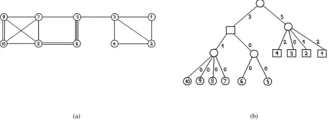
sum of the demands of its children. For an illustration of an extreme-sets tree and an extreme-sets partition see Figure 1.
For a graphG0and for any vertexvinG0, we denote byXv(G0)the set inES(G0)that containsv. When
G0 =Gwe use the shorthandsX
v andES, respectively.
2.3 k-Connectivity (k > 1): the Algorithm
When approximating the distance to1-connectivity the algorithm estimates, for every vertex selected, the
size of its connected component. In an analogous way, in order to approximate the distance tok-connectivity,
which equals to 1
mdφ(ES)/2ewhere φ(ES) =
P
v∈V φ(Xv)
|Xv| , we estimate for every vertexvthe demand
and the size ofXv. More precisely, sinceXv may be large for some vertices, we introduce a certain refine-ment ofESthat consists of subsets of a bounded size.
Definition 3 Given a graphGand a size boundt, thet-bounded extreme-sets partitionis the partition
ES(t) =ES(t)(G) ={X(t)
1 , . . . , X (t)
q }that satisfies the following conditions: 1. For everyi, the size ofXi(t)is at mostt.
(a) (b)
Figure 1: (a) A graph and (b) its extreme-sets tree and extreme-sets partition. Each node represents an extreme set. The values on the edges are the demands of the corresponding extreme sets fork = 4. The squared nodes represent
the sets of the extreme-sets partition.
2. For everyi,Xi(t)is an extreme set with the property that eitherφ(Xi(t)) = 0or
φ(Xi(t))>P
Y<X(t)
i
φ(Y).
3. For everyi, Xi(t) is not contained in any other extreme set of size at mosttsatisfying Conditions 1 and 2.
We claim that φ(ES) ≥ φ(ES(t)) . To verify this, note that the sets ofES whose size is at mostt
are also sets ofES(t). The other sets of ES are further partitioned inES(t) into smaller sets that satisfy
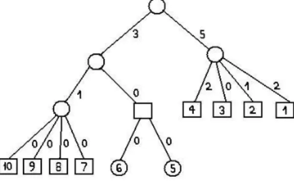
Conditions 2 and 3 of Definition 3. That is, every set inESwhose size is larger thantis replaced inES(t) by smaller extreme sets from its subtree. Now, by the definition of the demand of a set (Equation (2)), the demand of every extreme set in the extreme-sets tree is always greater or equal to the sum of the demands of its children, therefore, the sum of demands of the sets inES(t)that replace some set inESis at most the demand of that set. For an illustration of at-bounded extreme-sets partition see Figure 2.
For any graph G0 and a vertex v inG0, we denote the set in ES(t)(G0) that contains v by X(t)
v (G0). WhenG0 =Gwe use the shorthandsES(t) andXv(t), respectively.
The following procedure searches for Xv(t) given a size bound tand a repetition parameter r, both of which will be set subsequently. It uses thecontractionoperation of a setAof vertices in which the vertices
ofAare merged into a single vertexaand for every edge(v, u)such thatv∈Aandu /∈A, there is an edge
Figure 2: The extreme-sets tree of the graph in Fig 1(a), and thet-bounded extreme-sets partition fort = 3. Each
node represents an extreme set. The values on the edges are the demands of the corresponding extreme sets fork= 4.
The squared nodes represent the sets of the3-bounded extreme-sets partition.
Procedure 1 (Extreme-set search from a given vertexv) 1. Repeat the following process for everyi= 1, . . . , r.
(a) (Random Search Process) Start withSi = {v}. As long as|Si| ≤tand the size of the cut(Si, Si)is less than3t2β, assign a random cost in the range[0,1]to the edges of the cut(Si, Si)that were not yet assigned costs. Traverse the edge of lowest cost and add the new vertex reached toSi.
(b) (Extreme-Set Search) LetGSi be the graph obtained from Gby contracting the set Si
to a single vertex si. Construct the extreme-sets tree of GSi and let X
Si
v be the set
Xv(GSi).
2. LetXvmax be the maximal set among{XSi
v }ri=1. DeclareXvmax as the set inES ofG con-tainingvi.e., asXv(t)(G).
Lemma 1 For everyvand size boundt, Procedure 1 findsXv(t)(G)with probability at least1−e−2r/t
2
. Its query complexity and running time areO(t4rβ3/2).
Proof: The construction of the extreme-sets tree of the graphGSi at Step 1.b, can be done by first
con-structing a hierarchical structure of the connectivity classes of GSi (called the class decomposition tree)
usingn−1max-flow computations [GH61, Gus90]. This takesO(˜nm˜3/2)time wheren˜=t+ 1is an upper
bound on the number of vertices inGSiandm˜ = (t+1)
2·βis an upper bound on the number of edges. Then, the classes that are not extreme sets are removed from the tree to get the extreme-sets tree [NGM97]. This is done usingO(˜nm˜)steps (see [NGM97] for more details). Thus the total running time for the construction
isO(t4β3/2). Step 1.a takesO(t3β)queries and time and therefore the total query and time complexity of
Procedure 1 isO(t4β3/2r).
To analyze the correctness of Procedure 1, assume first that at least one iteration of the random search process (Step 1.a) finds a setS that containsXv(t)(G). In the following claim we establish that in this case, the procedure declaresXv(t)(G)as the required set.
Claim 2 If at least one iteration of the random search process of Step 1.a finds a setSthat containsXv(t)(G), then Procedure 1 findsXv(t)(G).
Proof: Consider thei’th iteration and the setSithat is found in Step 1.a. Step 1.b consists of deterministic sub-procedures and therefore always findsXv(t)(GSi). Note that by the transition from the original graphG
to the graphGSi we do not necessarily preserve the connectivity of vertices inSi. The connectivity cannot
decrease but it might increase. However, we can easily show that the collection of all extreme sets that are contained inSi is exactly the same inGand inGSi. This follows immediately by observing that for every
setU ⊆Si, the degree ofU,d(U), is exactly the same inGand inGSi. Also, the demand of any extreme
set is a local property that depends only on its degree and its sub-extreme sets, thus, the demand of every extreme set that is contained inSi is exactly the same inGand inGSi. Therefore, since Step 1.b always
findsXv(t)(GSi), ifSicontainsX
(t)
v (G), thenXvSi =X
(t)
v (G). That is, at thei’th iteration, the extreme-set search of Step 1.b findsXv(t)(G).
Now, consider the collection{XSi
v }ri=1 of the sets found in iterations1, . . . , r. Assume w.l.o.g that the sets are ordered by an increasing order of their size. Then for every i,XSi
v ⊆ X Si+1
v . This follows from the fact that every two extreme sets are either disjoint or one is contained in the other and sincev ∈ XSi
v for every i. In addition, for everyi, XSi
v satisfies conditions 1 and 2 of t-bounded extreme sets. Thus all the sets except the largest one (or the few largest ones in case the largest set was found more than once) are contained in another extreme set that satisfies conditions 1 and 2 and therefore do not satisfy condition 3. We conclude that if some iteration foundsXv(t)then necessarilyXv(t)is the largest set among{XvSi}ri=1. What is left to analyze is the probability that the random search process of Step 1.a finds a setS
contain-ingXv(t). To this end we lower bound the probability that all the vertices ofXv(t) are added to the growing setS before any other vertex is. But first, observe that for everyS ⊆Xv(t), the size of the cut(S, S)is less than3t2β. Thus, if the algorithm adds toS only vertices fromX(t)
v , it won’t stop before all the vertices of
Xv(t)are inS. To verify this, for every v∈Xv(t) let dinv denote the degree ofvin the subgraph induces by
Xv(t)(dinv is less thantβ) and let doutv =dv−dvin. Consider any vertexu∈Xv(t). SinceXv(t)is an extreme set, Pv∈X(t)
v d
out
v < du < doutu +tβ. In other words,
P
v∈Xv(t)\{u}d
out
v < tβ . Since this is true for every
u∈Xv(t), the size of the cut(Xv(t), Xv(t)), which equals to Pv∈X(t)
v d
out
v , is less than2tβand thus for every
S ⊆Xv(t) , the size of the cut(S, S)is less thant2β+ 2tβ ≤3t2β. Note that the algorithm cannot detect the point at whichS=Xv(t)since the value of`, such thatXv(t)is`-extreme, is unknown.
Now, consider the graphGX obtained fromGby contracting the setXv(t)into a single vertexx. Assume that the random search process of Step 1.a runs onGX fort0 =|Xv(t)|steps. The cut(Xv(t), x)is a minimum cut ofGXsinceXv(t)is an extreme set. Goldreich and Ron proved in [GR02] that in this case the probability that no cut edge is traversed beforeXv(t)is found is at least2t−2. Their analysis is based on Karger’s analysis of his algorithm for finding minimum cut in a graph [Kar93].
Lemma 3 [GR02] For an undirected graphG, letLbe a set of at mosttvertices such that the cut(L, L)is a minimum cut. Then, starting with some vertexv ∈L, the random search process of Step 1.a succeeds in finding the cut(L, L)with probability at least2t−2.
Proof Sketch: Consider the graph GL obtained from Gby contracting the set L into a single vertex `. Assume that the edges ofGLare randomly and independently assigned costs in the range[0,1]and that the
random search process runs onGL. Observe that if the subgraph induced onLcontains a spanning tree that is cheaper than the cut(L, `)(i.e., the cost of every edge of the spanning tree is smaller than that of any cut
edge) then the random search process findsL. This is true since in this case, at every step there is some edge
whose cost is cheaper than the cost of any cut edge, thus no cut edge is traversed. To analyze the probability that such a spanning tree exists, consider the Contraction Algorithm of Karger for finding a minimum cut in a graph [Kar93]. At every step of his algorithm, the edge with the smallest cost out of the remaining edges in the graph is contracted (as opposed to the smallest cost cut edge in our algorithm). The process continues until one edge remains. Karger showed that for every fixed minimum cut, the probability that no cut edge is contracted is at least2t−2. The contracted edges form 2 spanning trees, attached to the endpoints of the
remaining edge, thus proving that in our case, the subgraph induced onLcontains a spanning tree that is
cheaper than the cut(L, L). This completes the proof. 2
Corollary 4 If we repeat the random search processrtimes, then, with probability at least 1−(1−2t−2)r>
1−e−2t−2·r
, at least one iteration finds a set containingXv(t).
Combining Corollary 4 with Claim 2, with probability at least1−e−2t−2r
, Procedure 1 findsXv(t), thus proving Lemma 1.
We now present the distance approximation algorithm that uses Procedure 1 to estimate the distance of a connected graph from beingk-connected.
Algorithm 2 (Distance approximation tok-connectivity)
1. Uniformly and independently sample s = 32k2/(δ2d¯2) vertices from G. Let S = {u1, . . . , us}be the multiset of the sampled vertices.
2. For every sampled vertex uj, run Procedure 1 using the size bound t = 4k/δd¯and the repetition constantr=t2ln(32δ2dk¯22). LetX be the extreme set found and letnbj =|X|.
3. Calculate the demand ofX and denote it byφbj.
4. Let φb= ns Psi=1 φbj b nj , let Cb= lb φ 2 m and output m1Cb.
Theorem 2 For everyk >1, Algorithm 2 is a distance approximation algorithm fork-connectivity of con-nected graphs. The query complexity and running time of the algorithm areO (k/(δd¯))6β3/2log(k/(δd¯)). As noted previously, in the full version of this paper [MR06] we show how to deal with the case of uncon-nected graphs. The only difference is a slight modification in Procedure 1.
Proof: Since the query and time complexity of Procedure 1 isO(t4·r·β3/2), and since the demand of the
setX found by the procedure is computed in the course of the procedure, the query and time complexity of
Algorithm 2 isO(s·t4·rβ3/2) =O (k/(δd¯))6β3/2log(k/(δd¯)), as claimed.
LetES = {X1, . . . , Xq}be the extreme-sets partition of Gand letES(t) = {X1(t), . . . , X (t)
q } be its
t-bounded extreme-sets partition fort= 4k/δd¯. Assume w.l.o.g that the sets are sorted by increasing order
of their size. Let`be the maximal index such that|X`| ≤t. ThenXi(t) =Xifor everyi≤`. Now, as noted before,φ(ES)≥φ(ES(t))so φ(ES)−φ(ES(t)) = p X i=j+1 φ(Xi)− q X i=j+1 φ(Xi(t)) (3)
≤ p X i=j+1 φ(Xi) ≤ δdn¯ 4k ·k = δ 2m. (4)
where the last inequality is true since there are at most n
t = 4k/δnd¯sets of size greater thantand the demand of any set is at mostk.
We next show that with high probability φbis a good estimate for φ(ES(t)). We first calculate the
probability that Procedure 1 succeeds in findingXv(t)for all the sampled vertices. For every sampled vertex
uj, as shown by Lemma 1, the probability that Procedure 1 fails to findXu(tj) is at moste−2t
−2·r
. Thus the probability that it fails for somejis at most
s X i=1 e−2t−2·r = s·e−2 ln(32k 2 δ2 ¯d2) < 32k2/(δ2d¯2)· (δ2d¯2)/(32k2)2 < 1 6. (5)
That is, with probability at least5/6, the procedure findsXu(tj)for every sampled vertexuj. Let nv =|X
(t)
v | and letφ(v)be the demand ofXv(t). Then, with probability at least5/6, for every sampled vertexuj,
b φj b nj = φ(uj) nuj .
Assuming this is true, for everyj, χj =
b
φj
b
nj is a random variable whose expected value is
1 n P v∈V φ(v) nv .
Let µ= Exp[k1χj]for somej. Then,
φ(ES(t)) = q X i=1 φ(Xi(t)) = X v∈V φ(v) nv = k·n·µ . (6)
The random variable 1
kχjgets values in the range[0,1], thus by an additive Chernoff bound, with probability at least5/6, Prbφ−φ(ES(t))> δ 2m ≤ Pr 1 s s X j=1 b φj k·bnj − µ > δ 4kd¯ < 2·e−2sδ2d¯2/16k2 < 1 6 (7)
That is, with probability at least2/3, |φb−φ(ES(t))| < δ
2m . Theorem 2 follows by applying the triangle inequality.
2.4 k-Connectivity fork ≥ 2and non-connected graphs
The algorithm of [NGM97] for optimally increasing the connectivity of a graph does not handle the case in which the given graph is not connected. We show, however, that it can be generalized to include this case also and state here the needed modifications.
Naor, Gusfield and Martel [NGM97] presented an algorithm that increases the connectivity of a given
λ-connected graph tok, by adding exactly dφ(ES)/2e edges. This number of edges matches the lower
bound discussed before, thus proving optimality. Their algorithm works ink−λphases, each increases the
connectivity of the graph by one. They prove that for every phasei∈ {1, . . . , k−λ−1}, if`iis the number of edges added, then the demand is decreased by2`i. In the last phase, since at most one endpoint is added
without satisfying a demand, the demand is decreased by either2`k−λor2`k−λ−1. The way the edges are selected is by first selecting pairs of extreme sets to connect using a graph structure calledcactusand then selecting the vertices inside the extreme sets, connecting them by an edge.
We focus on the first phase in which the connectivity of a graph G withp connected components is
increased to1. We describe how to choosep−1edges so thatGwill become1-connected and the demand
φ(ES)will be decreased by2(p−1). Consider the graphG0 obtained by contracting every2-class ofG
into a single node. G0 is a forest ofptrees where each tree consists of one or more nodes. LetT
1, . . . , Tp be the trees of G0. IfTi consists of one node then it corresponds to a 2-class of G, otherwise, its leaves correspond to1-extreme sets ofG. For everyi, choose two arbitrary leavesui1 andui2 in the treeTi. For trees of only one node, choose this node twice. For everyi∈ {1, . . . , p−1}match the pair(ui2, u(i+1)1). Then, ifui1 =ui2(the treeTiconsists of one node) choose two vertices in the corresponding2-class ofTi, otherwise, choose one vertex in the corresponding extreme set of ui1 and one vertex in the corresponding extreme set of ui2. Now, for every pair(ui2, u(i+1)1)add an edge connecting the selected vertices in the corresponding extreme sets. The selection of those vertices is done using a similar rule to that defined in [NGM97]:
For every leafuij, letUij be its corresponding extreme set in the extreme-sets tree of G. If only one endpoint should be added to a vertex in Uij then find an extreme set Wij in the subtree ofUij such that
φ(Wij)>0andφ(Z) = 0for everyZchild ofWij. Then choose an arbitrary vertex inWij. If on the other hand two endpoints should be added to vertices inUij then there are two cases: IfUij is ak-class, select two arbitrary vertices inUij(unless it contains only one vertex, in which case this vertex is selected twice). Otherwise, find two extreme setsWi1andWi2in the subtrees of two separated children ofUijsatisfying the same rule as in the case where only one endpoint should be selected. Then choose two arbitrary vertices, one inWi1 and the other inWi2
We claim that the addition of suchp−1edges toG, which clearly increase the connectivity ofGby1,
decrease the demandφ(ES)by2(p−1). The proof is similar to the proof for the other phases in [NGM97].
The only difference is the proof for Lemma 4.5 of [NGM97] that in our case follows immediately from the construction. We refer the reader to [NGM97] for more details. This ensures that when combining the rest of the phases as described in [NGM97], the total number of edges added isdφ(ES)/2e and the resulting
graph isk-connected. Thus, if the given graph is not connected, its distance fromk-connectivity, fork ≥2
is exactly 1
dndφ(ES)/2eas for a connected graph.
As for the implications on our algorithm, Procedure 1 has to be modified in the following way. Whenever the Random Search Process of Step 1.a finds the connected componentCvofv, the extreme-sets tree ofCv is built and the procedure declares the setXv(Cv)asXv(G). Note thatXv(Cv)is exactlyXv(G)so that if
vbelongs to a small connected component, the procedure always findsXv(G).
3
Distance Approximation to Subgraph-Freeness
For a fixed graphH, we say thatGisH-free if it contains no subgraph isomorphic toH. In this section we
consider the problem of approximating the distance of a graph from beingH-free for some fixed subgraph Hin the bounded-degree model. We note that testing subgraph-freeness in the general sparse model requires
Ω(√n)queries [AKKR06].
In what follows we focus on triangles and then generalize the result to arbitrary subgraphs (in Subsec-tion 3.2). We first present a non-sublinear algorithm for approximating the minimum number of edges that should be removed in order to obtain a triangle-free graph. Later we show how to transform it into a distance approximation algorithm whose running time is independent ofn.
3.1 Triangle-Freeness
LetGbe an undirected graph with degree at mostd and letm = dn. We say that two triangles inGare
neighbors if they share a common edge. For a triangle t, the set of its neighboring triangles is denoted
by Γ(t). The degree of a triangle, denoted byd(t), is defined as the size of Γ(t). Thedistance between two trianglestand t0 is the minimum number of triangles minus1in a sequencet1, . . . , t` of triangles for whicht1 = t andt` = t0 and for everyi ∈ {1, . . . , `−1}, the triangles ti and ti+1 are neighbors. The
k-neighborhood of a triangletis defined as the set of triangles whose distance fromtis at most k. In an
analogous way, thek-neighborhood of a vertexvis the set of vertices whose distance fromvis at mostk.
For a setSof edges, we say thatSis atriangle coverif its removal from the graph results in a triangle-free graph and denote byCOP T the minimum size of a triangle cover ofG.
The following algorithm gets as input a graphGwith degree at mostdand a parameterδ, and
approxi-matesCOP T.
Algorithm 3 (Minimum triangle cover approximation)
1. LetT be the set of all the triangles inGand letT C=∅be the initial triangle cover. 2. Fromi= 1to r = Θ(log(d/δ))
(a) Select each trianglet ∈ T with probability c·d1(t) , wherecis some constant that will be defined later. Ifd(t) = 0thentis selected with probability1.
(b) Un-select every two neighboring triangles that were selected. (c) Add all the edges of the selected triangles toT C.
(d) Remove fromT all the selected triangles and their neighbors and update the degrees of the remaining triangles accordingly.
3. Add toT Cone edge of every remaining triangle inT. 4. OutputT C.
Theorem 3 For everyδ, Algorithm 3 constructs a triangle coverT Cof sizeCsuch that with probability at least5/6, COP T ≤ C ≤ 3·COP T + δm2 .
Proof: First it is clear thatT Cis indeed a triangle cover and thereforeC ≥ COP T.
To show that C ≤ 3·COP T + 12δm consider first the triangles that the algorithm adds to the cover during the loop of Step 2. Observe that these triangles are all edge-disjoint since whenever the algorithm selects neighboring triangles in Step 2.a, it un-selects them in Step 2.b. Also, any neighbor of a selected triangle is removed fromT and cannot be selected on the following iterations. Therefore, any other triangle
cover must contain at least one edge of every triangle fromT Cso the number of edges added toT Cduring
the loop is at most3·COP T.
In order to upper bound the number of triangles left inT at the end of the loop of Step 2 we apply the
following lemma.
Lemma 5 For every i ∈ {1, . . . , r} let Ti be the number of triangles left in T at the end of the i’th iteration of Step 2. For i= 0 let Ti =|T |. Then for every i >0,
Exp [Ti |Ti−1]≤ 1− 1 c1 Ti−1
where c1 = 3c2/(c−3) and c is the constant used in Step 2.a of Algorithm 3.
Proof: For every iterationiand degreej ∈ {0, . . . ,3d}, let Ti,j be the number ofj-degree triangles left inT at the end of thei’th iteration so that Ti =Pj3d=0Ti,j . At Step 2.a, every triangletof degreej >0 is selected with probability1/(cj)and is un-selected in Step 2.b only in case at least one of its neighbors is
also selected. To calculate the probability that at least one neighbor oftis selected, letΓk(t) be the set of
t’s neighbors at itsk’th edge fork ∈ {1,2,3}, and letdk(t)be the size ofΓk(t). Then, the probability that at least one oft’s neighbors is selected is at most
X t0∈Γ(t) 1 c·d(t0) = 3 X k=1 X t0∈Γ k(t) 1 c·d(t0) ≤ 3 X k=1 X t0∈Γ k(t) 1 c·dk(t) = 3 c (8)
where the inequality is true since for every t0 ∈ Γk(t), d(t0) ≥ dk(t). Hence, we expect that on each iteration the algorithm un-selects only a constant fraction of the selected triangles. Therefore, for everyj >
0, the probability that aj-degree triangle is added toT Cis at least 1
cj 1−3c
= c10j wherec0 =c2/(c−3). It follows that the expected number ofj-degree triangles that are added toT Con thei’th iteration is at least Ti−1,j/(c0j) . Such triangles are removed from T together with their j neighbors. So for every j > 0, we expect that the chosen j-degree triangles cause the removal of at least j·Ti−1,j/(c0j) = Ti−1,j/c0 additional triangles of some degree. The removal of a triangle can be caused by more than one selected neighbor, but since the selected triangles are all edge-disjoint, we counted every removed triangle at most three times. Forj= 0, all theTi−1,0 triangles of degree0are selected and removed fromT. Summing up and canceling the repetitions, the expected total number of triangles removed fromT at thei’th iteration
is at least (1/3)P3jd=0Ti−1,j/c0 = (1/c1)Ti−1 wherec1 is as defined in the lemma, and the proof of the lemma is completed.
The next corollary follows from Lemma 5.
Corollary 6 By takingc= 6, after r= 36(log(dδ) + 3) iterations,Exp[Tr]≤ 12δd|T |. Proof: It follows from Lemma 5 that for everyi >0,
Exp[Ti] = X a∈{0...|T |} Exp[Ti|Ti−1=a]·Pr[Ti−1=a] (9) ≤ X a∈{0...|T |} 1− 1 c1 ·a·Pr[Ti−1 =a] (10) = 1− 1 c1 Exp[Ti−1] (11)
and therefore by simple induction Exp[Tr] ≤
1− 1
c1
r
|T | .Now c1 is minimal whenc = 6, in which case it equals36and so,
Exp[Tr]≤ 1− 1 c1 c1·(log(dδ)+3) |T |<exp(−log(d δ) + 3)· |T |< δ 12d|T | (12) as required.
Using Markov’s inequality, the probability that Tr > 2δd|T |is less than 1/6. Now, since every edge belongs to at mostdtriangles, we have |T | ≤dmand so with probability at least5/6the number of edges
added to the coverT Cin Step 3 is at most 12δm. We conclude that in this case, the size of the cover is upper bounded by3·COP T +12δm, which completes the proof of Theorem 3.
Next we show how to modify Algorithm 3 in order to achieve a 3-distance approximation algorithm
for triangle-freeness whose running time is independent of n. Specifically, the algorithm uniformly and
independently selectsΘ(1/δ2)vertices and then for each triangle attached to a sampled vertex, determines
whether or not it would have been added toT Cby Algorithm 3. This can be determined by examining only
theΘ(log(d/δ))-neighborhood of every sampled vertex.
Algorithm 4 (Distance approximation to triangle-freeness)
1. Uniformly and independently samples = 2/δ2 vertices fromG. Let S ={u
1, . . . , us} be the multiset of the sampled vertices.
2. For everyj ∈ {1, . . . , s}observe the subgraphGr(uj)induced by the(r+ 1)-neighborhood ofuj, wherer= Θ(logdδ)is as in Algorithm 3.
3. Run Algorithm 3 on Ssj=1Gr(uj). For everyuj ∈S, letχjbe the number of edges incident toujthat the algorithm adds to the cover.
4. Let Cb= 2nsPjs=1χj and output dn1 Cb.
Theorem 4 Algorithm 4 is a3-distance approximation algorithm for triangle-freeness. The query complex-ity and running time of the algorithm aredO(log(d/δ)).
Proof: The claimed complexity of the algorithm can be easily verified. To prove the quality of the estimate, we fix the random bitsτthat Algorithm 3 uses and assume that Algorithm 4 uses the sameτ when executing
Algorithm 3 in Step 3. LetT Cτ be the cover found by Algorithm 3 when usingτ and letCτ be its size. For every vertexvletxτv be the number of edges incident tovinT Cτ. In addition, letCbτ be the output of
Algorithm 4. Cbτ is an estimate toCτ. For everyj, letχτj be the value ofχj when usingτ. We will show that for every sampled vertexuj, the numberχτj calculated by Algorithm 4, exactly equalsxτuj. The only
error, therefore, is due to sampling which, as we will show, is not too large.
We first observe that at the end of every iteration of Algorithm 3, every triangle tcan be found in one
of the following three states. It might be added to T Cτ (and consequently removed fromT), it might be
removed fromT (without being added toT Cτ) and it might remain inT. In the following lemma we’ll
show that it is enough to observe the 2r-neighborhood of a triangle in order to determine its state afterr
iterations. From a vertex point of view, this implies that inspecting its(r+1)-neighborhood suffices in order
to determine the state of all the triangles incident to it afterriterations. To verify this, one can easily show
by induction onithat the(i+ 1)-neighborhood of a vertexvcontains the2i-neighborhood of the triangles
incident tov. The following claim implies, therefore, that for every sampled vertexuj,χτj =xτuj.
Claim 7 For every trianglet, it is enough to observe its2r-neighborhood in order to determine its state at the end of ther’th iteration of Algorithm 3.
Proof: We prove the lemma by induction on the iteration numberi. Fori= 1,tis added toT Cin case it is
selected and none of its neighbors are selected. It is removed fromT in case it is not selected and at least
one of its neighbors,t0, is selected while none oft0’s neighbors is. Otherwise it remains inT. So, in order
claim is true fori < r. Then for ther’th iteration, by the same argument, one needs to know the state oft’s
2-neighborhood at the end of ther−1iteration. That is, observing the 2(r−1) + 2 = 2r-neighborhood of tsuffice, as required.
Now, for everyj, χτ
j is a random variable whose expected value is n1
P
v∈V xτv . Let µτ = Exp[1dχτj] for some j. Thus, Cτ = 1
2 P
v∈V xτv = dn2 ·µτ . The random variable 1dχτj gets values in the range
[0,1]. By an additive Chernoff bound,PrSh bCτ −Cτ
> δ2dni<1/6. From Theorem 3 we know that the
probability over the possible sequences of random bitsτ, thatCτ is less than 3·COP T +δm2 is at least
5/6. Combining this and the fact thatm ≤ dn, we get that with probability at least2/3,COP T ≤ Cb ≤
3COP T +δdn. (Theorem 4)
3.2 Generalizing the Result to Arbitrary Subgraphs
The result for triangle-freeness can be generalized to arbitrary subgraphs using some subgraph specific parameters. Assume thatH consists ofmH edges and its diameter is ρH. Also, letdH be the maximal number of subgraphs a single edge can belong to. For trianglesdH =O(d)but for other subgraphs it might be much larger. For example, for the cycle of lengthd, an edge in a complete subgraph ofdvertices, belongs
to(d−2)!cycles of lengthd. For a fixed graphH,Gis calledH-freeif no subgraph ofGis isomorphic
toH. We say that a set of edges is anH-coverif its removal from the graph results in anH-free graph and
denote byHCOP T the minimum size of anH-cover of G. Two isomorphic copies of H inGare called neighborsif they share at least one edge. For an isomorphic copyhofH, the set of its neighbors is denoted
byΓ(h)and itsdegree,d(h), is defined as the size ofΓ(h). Using these definitions, Algorithms 3 and 4 can
be modified to compute the distance of a bounded-degree graph from beingH-free, for every fixed subgraph H.
Theorem 5 For every constant size subgraph H, there exists a variant of Algorithm 4 that is an mH -distance approximation algorithm for H-freeness. The query and time complexity of the algorithm is
dO(ρH·m2H·log(dH/δ)).
Proof Sketch: First we describe and analyze a variant of Algorithm 3 that constructs an H-cover ofG.
Let H be the set of all the subgraphs isomorphic to H at the beginning of the algorithm and for every
iteration i, let Hi be the set of subgraphs left in H at the end of the i’th iteration. At Step 2.a every subgraph h selects itself with probability 1/(c·d(h)). By the same analysis as that of Algorithm 3, it is
unselected at Step 2.b with probability at mostmH/cand therefore, for everyi, at thei’th iteration, at least
(1/c1)|Hi−1| subgraphs are removed from H. The constant c1 in this case equalsmHc2/(c−mH). By takingc= 2mH, afterr= 4mH2 (log(dH/δ) + 3)iterations, with probability at least5/6the number of the remaining subgraphs is at most δ
2dH|H|. Since every edge belongs to at mostdH subgraphs, |H| ≤ dHm.
Therefore, combining the fact that the number of subgraphs added to the cover during the loop is at most
mH ·HCOP T, with probability at least5/6, C≤mH ·HCOP T +12δm.
The adapted version of Algorithm 4 outputs an estimate to HC, the size of the H-cover T C. It can
be verified that for every fixed subgraph H, observing the 2r-neighborhood of some isomorphic copy h
of H suffices in order to determine its state at the end of the r’th iteration. Also, for every vertex, its
(ρH·(2r+ 1))-neighborhood contains the2r-neighborhood of every subgraph it belongs to. So by the same analysis, we get anmH-distance approximation forH-freeness.
The induced subgraph Gr(u) can be constructed using dO(ρH·m
2
H·log(dH/δ)) queries and so the total
query complexity is as claimed. As for the running time, there aredO(ρH·m2Hlog(dH/δ))vertices. For every
combinations of edges in itsρH vicinity, i.e., usingO(dρH·mH)steps. So, going over all the subgraphsO(r) times takesdO(ρH·m2H·log(dH/δ))steps. 2
3.3 Approximating the Minimum Vertex Cover
We observe that Algorithm 3 is readily seen to be a randomized distributed approximation algorithm. By ap-plying some modifications, it can yield a distributed algorithm for approximation the minimum vertex cover of a graph, which is one of the fundamental problems extensively studied in various settings in Computer Science. Details follow.
The distributed computation model consists of an underlying (synchronous) network G in which the
vertices represent processors and the edges represent the communication channels. A distributed algorithm runs ink rounds for some numberk, where in each round every vertex is allowed to send messages to its
neighbors. Afterkrounds, each vertex completes its computation and the entire network achieves this way
some global goal. For example, if the goal is to compute a vertex cover, then each vertex should decide whether or not it belongs to the vertex cover. In the local computation model, each vertex performs its task based on local information only, that is, k is smaller than the diameter of the graph. Usually there is a
trade-off between the locality of the algorithm and the quality of the solution.
For completeness we present the distributed version of Algorithm 3 for the minimum vertex-cover prob-lem. We start with some definitions. Two edges are considered neighbors if they share a common vertex. For an edgeewe denote byΓ(e)the set of its neighbors and byd(e)the size ofΓ(e). We denote byV COP T the size of a minimum vertex cover. The following is a randomized distributed algorithm the finds a vertex cover whose size is at most(2 +δ)times the minimum size with high constant probability.
Algorithm 5 (Distributed approximation for minimum vertex cover) 1. Every edge activates itself.
2. Fromi= 1to r = Θ(log(d/δ))
(a) Every active edgeeselects itself with probability 4·d1(e). Ifd(e) = 0thene
is selected with probability1.
(b) Every two neighboring edges that were selected, unselect themselves. (c) Every vertex that is attached to a selected edge, adds itself to the vertex
cover.
(d) Selected edges and neighbors of selected edges, inactivate themselves. (e) Active edges update their degrees to be the number of their active neighbors. 3. One vertex of every still active edge, adds itself to the vertex cover.
Theorem 6 For everyδ > 0and every graphG= (V, E)with degree-bound d, Algorithm 5 constructs a vertex cover C ⊆ V such that with probability at least 5/6,V COP T ≤ |C| ≤ (2 +δ)·V COP T The query complexity and running time of the algorithm aredO(log(d/δ)).
The proof is very similar to the proof of Theorem 3, and hence we only give a sketch. Proof Sketch: Since an edge inactivates itself only when one of its endpoints is added to the vertex cover, and in Step 3 one end-point from each edge that is still active is added to the cover, all edges are covered by the end of the algorithm, as required. This implies also the lower bound on|C|.
Analogously to the proof of Theorem 3, with probability at least5/6, at the end of the Step 2, the number
of inactive edges is at most δ
2d|E|. Since the degree of every vertex is at mostdand at leastV COP T vertices must be selected in order to cover all the edges, we have |E| ≤d·V COP T . Combining this with the fact that the number of vertices selected during Step 2 is at most 2·V COP T we have, |C| ≤ (2 +δ)V COP T.
2
3.3.1 A Sublinear Approximation of the Size of a Minimum Vertex Cover
The problem of approximating the size of a minimum vertex cover has been studied also in the context of sublinear algorithms. Parnas and Ron [PR05] show a reduction from local distributed approximation algorithms to sublinear algorithms. Using the distributed algorithm of Kuhn, Moscibroda and Watten-hofer [KMW06] mentioned in the introduction, their reduction gives an approximation with a multiplicative factor of2and an additive factor ofδn, in time dO(δ−3·log(d)). The dependence on the maximum degreed
can be replaced by a dependence on Θ( ¯d/δ) . Algorithm 4, when modified to approximate the size of the
minimum vertex cover, obtains an estimate of the same quality in timedO(log(d/δ)). It can also be viewed as a reduction from Algorithm 5. For completeness we describe the modified algorithm.
Algorithm 6 (Sublinear Approximation forV COP T)
1. Uniformly and independently sample s = 4/δ2 vertices from G. Let S be the multiset of the sampled vertices.
2. For every v ∈ S, observe the subgraph Gr(v) induced by the (r + 1) -neighborhood ofv, wherer= Θ(log(dδ))is as in Algorithm 5.
3. Run Algorithm 5 on Sv∈SGr(v) (in a sequential manner). For everyv∈S, let
χv = 1if the algorithm addsvto the cover, otherwiseχv = 0. 4. Output V Cd= ns Pv∈Sχv .
The proof is analogous to the proof of Theorem 4 and is ommitted.
Theorem 7 For every δ > 0, and every graph G, Algorithm 6 outputs with probability at least 2/3 an estimateCbthat satisfies
V COP T −δn ≤ V Cd ≤ 2·V COP T +δn . The query and time complexity of the algorithm are dO(log(d/δ)).
We remark that the same modifications of the algorithm in [PR05] can be applied here to achieve a depen-dence on Θ( ¯d/δ) instead ofdin the running time and query complexity.
4
Distance Approximation to Being Eulerian
A graphGis Eulerian if there exist a path in the graph that traverses every edge ofGexactly once. It is a
well known fact that a graph is Eulerian if and only if it is connected and all vertices have even degree or exactly two vertices have odd degree. Goldreich and Ron [GR02] gave a testing algorithm for this property in bounded-degree graphs, where the complexity of the algorithm is roughly linear in1/. The algorithm
can be easily adapted to general sparse graphs at a slight increase in the complexity. Here we give a distance approximation algorithm for general sparse graphs.
Algorithm 7 (Distance approximation to being Eulerian)
1. Run the following variant of Algorithm 1: The sample size is δ1282d¯2, the size bound is
8
δd¯and for every sampled vertexv, if its connected component was found and all the vertices in this component are of even degree thennbvis the number of vertices in this component, otherwise,
b
nv =∞. LetCbebe the estimate of the algorithm for the number of connected components. 2. Uniformly and independently samples = 16
δ2d¯2 vertices fromG. LetS be the multiset of the
sampled vertices.
3. Query the degreedj of every sampled vertexuj ∈S.
4. For everyj ∈ {1, . . . , s}, ifdj is odd then let χj = 1 otherwise let χj = 0. 5. Let Rb= 2nsPsj=1χj+Cbe−1 and outputR/b ( ¯dn)
Theorem 8 For everyδ >0and every graphGovernvertices and average degree d¯, with probability at least2/3, Algorithm 7 outputs a estimate to the distance ofG from being Eulerian. The query and time complexity of the algorithm isO((δ·d¯)−4β).
Proof: Consider the connected components of G. In each connected component, either all vertices have
an even degree or there is a positive even number of vertices with an odd degree. In the former case we refer to the component as aneven-degreecomponent, and in the latter case we refer to it as anodd-degree component. LetCedenote the number of even-degree components, and for each vertexvletxv = 1ifvis an odd-degree vertex, and letxv = 0otherwise. We claim that the minimum number of edges that must be added toGin order to make it Eulerian is 12·Pv∈V xv+Ce−1.
It is easy to verify that these many edges suffice to make the graph Eulerian. To show that this number is necessary consider first the process of adding any Ce+Co −1 edges that make the graph connected. Such a process necessarily leaves us with at least Pv∈V xv−2Co+ 2odd-degree vertices. To verify this observe that the addition of the edges defines a tree, whose nodes are the connected components. Let k
be the number of leaves in this tree that correspond to even-degree components (where k ≥ 0). Each
such leaf contributes an odd-degree vertex, and “uses”k end-points among theCe+Co−1added edges. Every even-degree component that does not correspond to a leaf “uses” at least2additional edges. Hence,
the remaining number of end points, which are attached to vertices in odd-degree components, is at most
2(Ce+Co−1)−(k+2(Ce−k)) = 2Co+k−2. Therefore, the number of odd-degree vertices that remain in odd-degree components is at leastPvxv−(2Co+k−2). Adding to this the (at least)kodd-degree vertices that belong to the even-degree components, we get at leastPvxv−2Co+ 2remaining odd-degree vertices.
So the total number of edges required is at leastCe+Co−1+21· Pv∈V xv−2Co= 12·Pv∈V xv+Ce−1 as claimed.
Now, Algorithm 1 with the modifications described in Step 1 of Algorithm 7, estimates the number of small connected components in which all the vertices are of even degree. As proved in Theorem 1, using the modified parameters, with probability at least5/6, |Cbe−Ce|< δ2m. In addition, using an additive Chernoff bound, with probability at least5/6, |ns
Ps
j=1χj − P
v∈V xv| < δ2m , and the claimed approximation is obtained.
The query and time complexity of Algorithm 1 (Step 1 of Algorithm 7) is O((δ ·d¯)−4β). The rest of
Algorithm 7 takesO((δ·d¯)−2)queries and time. Thus the total query and time complexity isO((δ·d¯)−4β).
5
Distance Approximation to Cycle-Freeness
The cycle-freeness property has been shown by Goldreich and Ron [GR02] to be testable in bounded-degree graphs in running time that is independent ofn. In the general sparse model, testing this property requires
at leastΩ(√n)queries. To verify this, consider2families of graphs, each consisting of all then!labelings
of the following twon-vertex graphs. The first is the empty graph and the second consists only of a clique
of size √nso that its distance to cycle-freeness isΘ(n). In order to distinguish between graphs that are
selected uniformly from each of the two families, a testing algorithm must perform at leastΩ(√n)queries.
In this section we give a distance approximation algorithm for this property for bounded-degree graphs. LetGbe a simple graph with degree-boundd, and letC1, . . . , Ck be the connected components ofG. For everyiwe define the number ofextraedges inCi byxi =mi−(|Ci| −1)wheremi is the number of edges inCi. The distance ofGto cycle-freeness equals therefore toX =Pki=1xi. The following algorithm approximates this number up to an additive factor ofδdnfor every givenδ >0and every bounded-degree
graph.
Algorithm 8 (Distance approximation to cycle-freeness)
1. Uniformly and independently samplet = 32δ2 vertices fromG. Let S = {u1, . . . , ut}be the multiset of the sampled vertices.
2. For everyuj ∈S, perform a BFS starting fromujuntilb= δd2 vertices have been reached or
uj’s connected component has been found.
3. For everyj∈ {1, . . . , t}, letbnj be the number of vertices visited and letxbj be the number of extra edges inuj’s connected component in case it was found, otherwisexbj = 0. Letdj be the degree of uj and also, letyj = 1ifuj belongs to a connected component of size larger thanb, otherwiseyj = 0. 4. Let Xbs= nt Ptj=1 b xj b nj , mb`= n 2t Pt
j=1dj·yj and bn`= nt Ptj=1yj . (‘s’ stands for ‘small’ and ‘`’ for ‘large’.) Let Xb =Xbs+mb`−bn` and output dn1 Xb .
Theorem 9 For everyδ > 0and every graphGonnvertices and maximum degreed, with probability at least2/3, Algorithm 8 outputs a estimate to the distance ofGfrom being cycle free. The query complexity