An Activity-Subspace Approach for Estimating the Integrated Input Function and Relative Distribution Volume in PET Parametric Imaging

An Activity-Subspace Approach for Estimating the

Integrated Input Function and Relative Distribution

Volume in PET Parametric Imaging

2_{Department of Electrical and Computer Engineering, University of British Columbia, Canada} 3_{Department of Electrical and Computer Engineering, University of Maryland, College Park, MD}

4_{Department of Radiology, Johns Hopkins University Medical Institutions, MD}

Abstract— Dynamic PET (positron emission

tomogra-phy) imaging technique enables the measurement of neu-roreceptor distributions corresponding to anatomic struc-tures, and thus allows image-wide quantification of phys-iological and biochemical parameters. Accurate quantifi-cation of the concentration of neuroreceptor has been the objective of many research efforts. Compartment modeling is the most widely used approach for receptor binding studies. However, current compartment-model based meth-ods often either require intrusive collection of accurate arterial blood measurements as the input function, or assume the existence of a reference region. To obviate the need for the input function or a reference region, in this paper, we propose to estimate the input function. We propose a novel concept of activity-subspace, and estimate the input function by the analysis of the intersection of the activity-subspaces. Then the input function and the distribution volume parameter are refined and estimated iteratively. Thus, the underlying parametric image of the total distribution volume is obtained. The proposed method is compared with a blind estimation method, Iterative Quadratic Maximum-Likelihood (IQML) via simulation, and the proposed method out performs IQML. The pro-posed method is also evaluated in a brain PET data set.

I. INTRODUCTION

The fundamental aim of functional imaging such as positron emission tomography (PET), single photon emission computed tomography (SPECT) is to extract quantitative information about physiological and bio-chemical functions (e.g. physiological parameters) from medical images. PET is a nuclear imaging technique relying on the unique physics of radionuclides that decay via positron emission. PET in dynamic mode can produce sequential images of in vivo distribution of a radioligand over time. PET imaging has found many clinical applications, with substantial contributions

to neurologic illnesses, oncology, and cardiovascular disease [1]. For example, using PET and a specific radioligand, the serotonin transporter (SERT) in the brain can be quantified to assess the integrity of serotonergic neurotransmission [2]. Of particular interest in this paper is the image-wide quantification of the concentration of neuroreceptor.

For the purpose of neuroreceptor quantification, the PET time-activity data are commonly analyzed by fitting to a mathematical model. Compartmental model-based approaches are the most widely used for tracer kinetic modeling in dynamic imaging [3], [4]. The compartmen-tal modeling approaches can be mainly classified into two categories, namely invasive and noninvasive, on the basis of whether arterial blood sampling is required. In the invasive approaches, a sequence of arterial plasma samples is used as the input function in the kinetic model [5], [6]. Though invasive models have some advantages, arterial plasma samples are often difficult to obtain or measure accurately, and such invasive mea-surement represents a limited, but not negligible risk of complications including thrombosis, infection and nerve injury [7]. Therefore, there has been increasing interest in noninvasive techniques.

Noninvasive techniques in the literature can be further classified depending on whether a reference region is needed. Examples of reference region based methods include [8] where the time activity curve (TAC) from carotid artery regions of interest (ROI) is used as the input function, and [9], [10] where a two-compartment model is assumed for the reference region. The reference region models obviate the need for input function by obtaining the parameters as a function of the reference region TAC. Another noninvasive research direction is to estimate both the kinetic parameters and the input func-tion simultaneously. For example, in [11], [12], the input

function is assumed to follow a mathematical formula, with several parameters to be determined. The param-eters for the input function and the kinetic paramparam-eters are estimated simultaneously through weighted nonlinear least square method. In [13], three blind identification schemes are examined and compared, namely the cross relations method (CR), the iterative quadratic maximum likelihood method (IQML) and the eigenvector-based algorithm (EVAM). These methods estimate kinetic pa-rameters without requiring the knowledge of the input function. The input function can be obtained based on the observed TACs and the estimated kinetic parameters. In this study, we revisit a novel noninvasive approach first proposed by our group [14], called the activity-subspace approach and also referred as intersectional searching algorithm (ISA) in [15]. The proposed activity-subspace approach does not assume any reference re-gions, and thus, falls into the category that estimates both the kinetic parameters and the input function. Compared with [11], [12], the proposed activity-subspace approach does not assume any mathematical structure of the input function. Different from the methods discussed in [13], the proposed approach first estimates the input function through the intersection of activity-subspaces. Then, with the estimated input function, the distribution volume parameters are iteratively estimated, and the estimated input function is refined at the same time. The basic idea is intuitively explained as follows. Since the TAC of each voxel is determined by the plasma input function and the dynamics of this voxel, it can be derived from the compartmental models that: for each voxel, a two-dimensional activity-subspace can be defined from its TAC; the integral of the input function belongs to the activity-subspace. It is noted that a common input func-tion is shared by all the voxels. Therefore, theoretically, given several different voxels and their corresponding activity-subspaces, the integral of the common input function belongs to all these different activity-subspaces, and thus can be estimated by finding the intersection of the activity-subspaces. Very recently, Naganawa et al proposed a method, called robust EPISA, for robust ex-traction of the cumulative integral of the input by jointly using ISA and clustering, and found successful applica-tions in real PET analysis [15]. It was shown that the cal-culated neuroreceptor images by the robust EPISA have a quality equivalent to that using the measured input after metabolite correction [15]. However, despite the promise of EPISA, there are still two disadvantages remained with the current activity-subspace based approaches: one is that it is shown to be sensitive to noise; the other is that the monotonicity of the estimated integral is not guaranteed. To overcome these two problems, in this

paper, we propose to use a novel clustering algorithm [16] jointly with the activity-subspace approach, which can efficiently reduce the noise in PET data. We also propose an iterative least square procedure that refines the estimated integral obtained by the activity-subspace approach, where the monotonicity of the estimated inte-gral is enforced in the iterative procedure.

This paper is organized as follows. In Section II, we first describe the models in the voxel domain, in-cluding the two-compartment model, three-compartment model and the graphical analysis (GA) plot of [17]; we then formulate the problem. In Section III, we present the proposed activity-subspace approach to estimate the input function and the parametric image of the total distribution volume. In Section IV, data simulations are put into operation. The performance of the proposed scheme is examined using brain PET data sets in Section V, followed by Discussions and Conclusions.

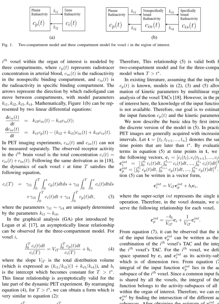
II. SYSTEMMODEL AND FORMULATION Accurate estimation of parametric images in neu-roreceptor studies often requires fitting the TACs to a mathematical model. Compartment models are the most popular models used for physiologically based quantification of the neuroreceptor concentration. In the literature, the in vivo tracer kinetics are often repre-sented by a serial compartmental model [3]. Measures such as binding potential (BP) and distribution volume (DV) are then often calculated based on the model parameters. A simple compartment model is the two-compartment model, as illustrated in Figure 1(a). The

ith _{voxel within the organ of interest is modeled by} two compartments. One compartment cp(t) represents the radiotracer concentration in arterial blood at time t, and the other represents radiotracer concentration in the tissue compartment ci(t). The two-compartment model can be mathematically written as a linear differential equation:

dci(t)

dt =ki1cp(t)−ki2ci(t), (1) where the rate constants ki1 and ki2 represents blood-tissue exchange parameters for the ith voxel. Equation (1) can be integrated and rearranged into the following form, Z _T 0 ci(t)dt= ki1 ki2 Z _T 0 cp(t)dt− 1 ki2ci(T). (2) Another widely used compartment model is the three-compartment model. For instance, in serotonin trans-porter imaging, brain regions containing receptors have the minimal number of three compartments. The three-compartment model is illustrated in Figure 1(b). The

(a) (b) Fig. 1. Two-compartment model and three compartment model for voxel iin the region of interest.

ith voxel within the organ of interest is modeled by three compartments, where cp(t) represents radiotracer concentration in arterial blood,cin(t) is the radioactivity in the nonspecific binding compartment, and cis(t) is the radioactivity in specific binding compartment. The arrows represent the direction by which radioligand can move between compartments, with model parameters

ki1, ki2, ki3, ki4. Mathematically, Figure 1(b) can be rep-resented by two linear differential equations:

dcis(t)

dt = ki3cin(t)−ki4cis(t);

dcin(t)

dt = ki1cp(t)−(ki2+ki3)cin(t) +ki4cis(t). In PET imaging experiments, cis(t) and cin(t) can not be measured separately. The observed receptor activity in the ith brain voxel is the total concentration ci(t) =

cis(t) +cin(t). Following the same derivation as in [18], the dynamics of each voxel i at time T satisfies the following equation, c_i(T) = γ_i1 Z _T 0 Z _s 0 cp(t)dtds+γi2 Z _T 0 Z _s 0 ci(t)dtds +γi3 Z _T 0 ci(t)dt+γi4 Z _T 0 cp(t)dt, (3) where the parametersγi1 ∼γi4 are uniquely determined by the parameters ki1 ∼ki4.

In the graphical analysis (GA) plot introduced by Logan et al. [17], an asymptotically linear relationship can be observed for the three-compartment model. For voxel i, R_T 0 ci(t)dt ci(T) =ViT R_T 0 cp(t)dt ci(T) +bi, (4) where the slope ViT is the total distribution volume (which is expressed as (ki1/ki2)(1 +ki3/ki4)), and bi is the intercept which becomes constant for T > t∗. This linear relationship is asymptotically valid for the late part of the dynamic PET experiment. By rearranging equation (4), forT > t∗, we can obtain a form which is very similar to equation (2):

Z _T

0 ci(t)dt=ViT

Z _T

0 cp(t)dt+bici(T). (5)

Therefore, This relationship (5) is valid both for the two-compartment model and for the three-compartment model when T > t∗.

In existing literature, assuming that the input function

cp(t) is known, models in (2), (3) and (5) allow esti-mation of kinetic parameters by multilinear regression analysis of the voxel TACs [18]. However, in the problem of interest here, the knowledge of the input functioncp(t) is not available. Therefore, our goal is to estimate both the input function cp(t) and the kinetic parameters.

We now describe the basic idea by first introducing the discrete version of the model in (5). In practice, the PET images are generally acquired with increasing time intervals. Let t ={tl, tl+1, ..., tn} denotes the sampling time points that are later than t∗. By evaluating the terms in equation (5) at time points in t, we define the following vectors, ci = [ci(tl), ci(tl+1), ..., ci(tn)]T,

cint i = [ R_tl 0 ci(t)dt, R_tl+1 0 ci(t)dt, ..., R_tn 0 ci(t)dt]T, and cint_p = [Rtl 0 cp(t)dt, R_tl+1 0 cp(t)dt, ..., R_t n 0 cp(t)dt]T. Equa-tion (5) can be written in a vector form,

cint_i =ViTcintp +bici, (6) where the super-script int represents the single integral operation. Therefore, in the voxel domain, we can ob-serve the following relationship for each voxel,

cint_p = −bi V_iTci+ 1 V_iTc int i . (7)

From equation (7), it can be observed that the integral of the input function cint_p can be written as the linear combination of the ith voxel’s TAC and the integral of the ith voxel’s TAC. For the ith voxel, we define the space spanned by ci and cinti as its activity-subspace, which is of dimension two. From equation (7), the integral of the input function cint_p lies in the activity-subspace of theith_{voxel. Since a common input function} is shared by all the voxels, the integral of the input function belongs to the activity-subspaces of all voxels within the organ of interest. Therefore, we can estimate

cint

p by finding the intersection of the different activity-subspaces. After obtaining the estimate of cint_p , we can apply iterative least square method to iteratively estimate

the kinetic parameters in equation (7) and refine the estimate of cint_p .

III. PROPOSED SCHEME

In this section, the proposed activity-subspace ap-proach is described in detail. In order to estimate the integral of the input function based on the noisy PET measurements, the problem of finding the intersection of different activity-subspaces is formulated as an op-timization problem. To reduce the noise effect, mixture principal component analysis (mPCA) [19] is employed to group the voxel TACs into several clusters. Since each cluster contains voxels with similar TACs and kinetic pa-rameters, the cluster average TAC will follow the model in equation (7). Through averaging, the noise effect is reduced. The activity-subspace approach will operate on the cluster average TACs, estimating the integral of the input function by finding the intersection between the activity-subspaces defined by cluster average TACs.

A. Activity-subspace intersection for estimating the in-tegral of the input function

In equation (7), assuming that ci and cinti are noise-free, we can see that the vectorcint_p lies in the subspace spanned by ci and cinti , which is defined as voxel i’s activity-subspace. For any two different voxels i and

j with different kinetic parameters, ideally the vector

cint

p should belong to both the activity-subspace spanned by ci and cinti and the activity-subspace spanned by cj and cint_j . Equivalently, in the ideal noise-free situation, the intersection of the two activity-subspaces is an one-dimensional subspace (a line), which defines the direc-tion of the vector cint_p . This observation motivates us to estimate the vector cint_p by exploring the intersection of the activity-subspaces.

Another observation is that, although the direction of the vector cint_p can be determined through the intersec-tion of activity-subspaces, we are not able to determine the length of the vector. In other words, we are able to estimate the shape of the curve R₀T cp(t)dt, but the amplitude remains unknown. As far as the distribution volume parametric image is concerned, not knowing the amplitude will not cause a problem. For example, if we determine the direction of the vector cint_p from the intersection of activity-subspaces and constraint the length of the vector to be 1, the estimated integral of input function ˆcint_p will be a scaled version of the integral of the true input function, i.e. ˆcint

p = ηcintp , where η is a scalar. If we use ˆcint_p to estimate the kinetic parameters in equation (6) using linear regression, the parameter bi will be estimated accurately, and the

estimated total distribution volume VˆiT will be scaled by a factor of 1_η, i.e. VˆiT = 1_ηViT. Since the estimated total distribution volume is scaled by the same factor for all voxels, the total distribution volume parametric image will not be affected. Therefore, in the proposed method, we constrain the estimated integral of the input function to be a vector of unit length, i.e., |ˆcint_p |= 1.

In practice ci(t)’s are noisy measurements, and thus the integral of ci(t) appears as a noise source too. The noisy nature ofci(t)certainly will affect the precision of the activity-subspace spanned byci and its integral cinti and thus the intersection of the activity-subspaces. As mentioned above, in the ideal noise-free case, the inter-section line between span(ci,cinti ) and span(cj,cintj ) defines the integral of the input function cint

p . How-ever, because of the measurement noise, both activity-subspaces are disturbed and the intersection line may no longer exist. Therefore, we propose to approximate the intersection by the following. In the ideal noise-free case, the intersection between span(ci,cinti ) and

span(cj,cintj ) can be equivalently regarded as a pair of lines, one in each activity-subspace, that share maximum correlation. Through a similar methodology, with the presence of measurement noise, we can find a pair of lines, such that one belongs to span(ci,cinti ), the other belongs to span(cj,cintj ), and this pair of lines share maximum correlation. The average of this pair of lines could be a reasonable approximation of the intersection line in the ideal case, which is the integral of the input function.

Mathematically, assume that vectors vi1 and vi2 are the ortho-normal basis of the subspace span(ci,cinti ). Then, any unit length vectorui inspan(ci,cinti ) can be written as,

ui =cos(θi)vi1+sin(θi)vi2 (8) where θi ∈ [0,2π). Therefore, the problem of finding the approximation of the intersection line between two activity-subspaces can be formulated as the following optimization problem, max θi,θj uT_iuj s.t.      ui=cos(θi)vi1+sin(θi)vi2 uj =cos(θj)vj1+sin(θj)vj2 θi∈[0,2π), θj ∈[0,2π) (9)

where, vi1 and vi2 are the ortho-normal basis of the activity-subspace span(ci,ciint), vj1 and vj2 are the ortho-normal basis of the activity-subspace

span(cj,cintj ). This maximization problem can be solved by grid search of possible values ofθiandθj over the range of [0,2π) (In the current implementation, the

grid search interval is 0.001, meaning that we examine

θi and θj that take any values which are multiples of 0.001). Assume θi = θ∗i and θj = θ∗j maximizes the objective, the corresponding ui(θ∗i) and uj(θ∗j) are the pair of lines, from activity-subspaces of voxel i and j, that maximize the correlation. Note that if ui(θi∗) and

uj(θ∗j) is the solution to the maximization problem in (9), so does −ui(θi∗) and −uj(θ∗j). We choose one of the two solutions based on the fact that the elements of

cint

p are all positive. If the number of positive elements is greater than the number of negative elements in vectors

ui(θ∗i) and uj(θj∗), the integral of the input function is approximated by ˆcint

p = 12(ui(θ∗i) +uj(θ∗j)). Otherwise, the integral of the input function is approximated by ˆ

cint

p = 12(−ui(θi∗)−uj(θ∗j)).

B. The clustering of voxels

To yield a fine approximation of the integral of the input function, it is desirable to reduce the noise level in the voxel TACs, which are used to define the activity-subspaces. To achieve this purpose, we cluster the voxels into several clusters according to their TACs. This idea is similar with working on the virtual regional TACs (e.g. each cluster represents a virtual regional TAC, which is not necessarily a spatially contiguous brain region). After clustering, each cluster is represented by the average TAC, based on which the cluster’s activity-subspace is defined. The integral of the input function can be estimated from the intersection of the activity-subspaces of different clusters.

Clustering voxels can be regarded as identifying dif-ferent voxel activity patterns, where each activity pattern can be represented by a different underlying model. As demonstrated in many areas, the idea of mixture Princi-pal Component Analysis (mPCA) has been a promising framework to deal with such problems by modeling the underlying nonlinearity and complexity with a mixture of local linear sub-models [16]. In our study, we propose to apply the mPCA approach for clustering.

The concepts in mPCA is related with the PET para-metric imaging problem as follows. In the mPCA ap-proach, a set of probabilistic PCA models is introduced by associating a probability density with the conven-tional PCA model. Assume there exist K clusters of functionally different voxels, whose activity patterns are different. mPCA describes each cluster by a probabilistic PCA model. The relative size of each cluster is modeled by a set of prior probabilities. Therefore, a voxel i, with probability p(k) (prior) belongs to the kth cluster, and thus can be represented by the kth probabilistic PCA model,

yi=Wkx+µk+²k, (10)

where yi is voxel i’s TAC. x is assumed to be an independent Gaussian vector with unit variance, x ∼

N(0, I)and dimensionq. The columns of the matrixWk are the q principal components of the activity pattern in the kth cluster. The principal components are not necessarily unitary, so that the energy of each component can be taken care of in theWkmatrix. The parameterµk represents the mean activity pattern, and ²k represents measurement noise. For the case of isotropic noise,

²k∼N(0, σi2I), the conditional probability of observing TACyi can be written as follows,

p(y_i|x, k) = (2πσ_k2)−d/2e− 1 2σ2 k kyi−Wkx−µkk2 . (11) Integrating the above equation over the distribution of

x, we obtain the distribution of observation yi given the

kth _{probabilistic PCA model,}

p(yi|k) = R p(yi|x, k)p(x|k)dx = (2π)−d/2_|C k|−1/2e− 1 2(yi−µk) T_C−1 k (yi−µk) (12) whereCk=σ2_kI+WkW_kT. Given the prior probabilities

p(k)of the set ofKprobabilistic PCA models, according to Bayes rule, the posterior probability of thekthmodel can be expressed as p(k|yi) = p(y_i|k)p(k) P_K k=1p(yi|k)p(k) . (13)

The posterior probability can be used for the purpose of clustering.

As in [19], an EM algorithm of mPCA is derived. In the E-step, given the observed TACs and model param-eters from previous iteration, the posterior probability of the kth model can be calculated. In the M-step, the model parameters are updated based on the previous model parameters and the posterior probabilities. The detailed EM algorithm is described in Appendix. When the algorithm converges, for each voxel, we obtain the posterior probability of the voxel belonging to each probabilistic PCA model conditioning on the observed TAC. Based on the posterior probabilities, voxels are grouped into clusters. For each cluster, the average TAC is calculated, based on which the activity-subspace of the cluster is defined. The integral of the input function is estimated from the intersection of activity-subspaces of different clusters, using the method described in section III-A.

C. Iterative least square for refining the estimated inte-gral

After voxel clustering, the integral of the input func-tion is estimated from the intersecfunc-tion of activity-subspaces defined by the clusters’ average TACs. We

extend the analysis to the voxel domain to further improve the accuracy of the estimated integral. Since each voxel TAC is a function of the same input function, we explore this property using the iterative least square method. For each voxeli, the noisy model of (6) can be expressed as, ci= −V_biT i cint_p +1 b_ic int i +ni = (cintp ,cinti ) µ_−ViT bi 1 bi ¶ +ni, (14) where the noise termni contains the measurement noise, the error from numerical integration, and the model mismatch error due to the asymptotically linear assump-tion. Define the observation matrix C = [c1, ...,cN],

S = [cint

p ,cint1 , ...,cintN ], the coefficient matrix A with

A(1, i) =−ViT/bi, A(i+ 1, i) = 1/bi and all other ele-ments being zero, and the noise matrixN= [n1, ...,nN]. Combining equation (14) of multiple voxels, we obtain the block formulation,

C=SA+N. (15) In order to estimate the kinetic parameters ViT, bi, the least-square (LS) formulation yields the following min-imization problem:

min

cint

p ,{ViT,bi}

||C−SA||2_F. (16) Searching for the global minimizer is computationally prohibitive even for modest number of voxels under consideration. To achieve an affordable computational cost, we apply the iterative least square method. The basic idea is that, we start from the initial estimate of

cint

p based on the intersection of activity-subspaces of voxel clusters, as described in sections A and III-B. Based on the estimated integral of input function, the coefficients in A can be estimated by least square regression. Using the estimate of A, which is the esti-mated {ViT, bi} for all voxels, the integral of the input function can be calculated from equation (7) for each voxel. The estimate of cint

p can be updated based on the calculated integrals from all the voxels. Note that, the initial estimate is obtained by the intersection of activity-spaces, where the monotonicity is not guaranteed. In the iterative least square procedure, the monotonicity can be easily enforced by updating cint

p based on the average of the calculated integrals that are monotonically increasing. The process iterates until convergence, when the difference between estimated cint_p in consecutive iterations is below a certain threshold.

The minimization problem in (16) has many local imizers. Therefore, in order to solve for the global min-imizer, a good initialization is required. In our scheme, the activity-subspace approach is employed to obtain the

initial estimate ofcint_p , which aims at finding the estimate ofcint_p that fits the activity-subspaces defined by several voxel clusters. We believe that such an initial estimate is naturally a good choice as it follows the underlying signal model. During the iterative least square procedure, we iteratively refine the estimate of the integral of the input function, the kinetic parameters are estimated at the same time. (Please note that, although we express the formulation in matrix form, the estimates are obtained in a voxel-by-voxel fashion.)

D. Summary of the proposed scheme

In summary the following steps are taken:

• Initialization: We apply the activity-subspace ap-proach to obtain the initial estimate of the integral of the input function. More specifically

– Preprocess time activity data and identify vox-els that belong to the brain region.

– Cluster the voxels TACs intoM clusters using Mixture Principal Component Analysis. A rea-sonable value of M should be chosen. Based on our observations, M = 2 could be a good choice. Denote the average cluster TACs asxj,

j= 1, ..., M, and their single integrals asxint_j . – For each pair (i, j), where i, j ∈ [1, M], the intersection of the activity-subspaces

span(xi,xinti ) and span(xj,xintj ) is obtained by (9). The intersections are the estimates of the integral of the input function. The average of them will serve as the initial estimate ofcint_p . • Iterative Refinement: With the initial estimate of

cint

p , the iterative least square is applied to further improve the estimation accuracy. At each iteration, – Given the estimatedcint_p from the previous iter-ation, for each voxeli, the coefficientsViT and

b_i are estimated using least square regression. – For each voxel, given the coefficients {ViT,

b_i}, the integral of the input function can be calculated from equation (7).

– The estimate ofcint_p is updated by the average of the calculated integrals that are monotoni-cally increasing. The estimate of cint_p is then normalized to a unit length vector.

– Iterate until convergence, the difference be-tween estimated cint_p in consecutive iterations is below a certain threshold.

Note that, if the data dynamic follows the two-compartment model, equation (6) holds during the entire experiment. In this case, t∗ = 0 and the integral of the input function during the entire experiment can be esti-mated. If the data follow the three-compartment model,

equation (6) is an asymptotic relationship which holds for the later duration of the experiment. In this case,

t∗ _{> 0, and for the integral of the input function, only} the time points later than t∗ can be estimated. The value oft∗ needs to be carefully chosen. The choice oft∗ is a trade-off between bias and variance. Since the graphical analysis (GA) plot is an asymptotical relationship for the later part of the PET experiment, if we choose a larger

t∗_{, equations (6) and (7) will better fit the TACs. On the} other hand, since only the time points after t∗ are used to define the activity-subspaces, largert∗ will reduce the available time points and thus decrease the robustness of the estimated activity-subspaces.

IV. SIMULATIONRESULTS

In the previous section, a novel idea of estimating the input function from activity-subspaces is proposed. In this section, we examine the performance of the activity-subspaces approach through simulation.

The time activities of two voxels are simulated by the three-compartment model. The kinetic parameters of the simulated voxels are k11 = 3.6247, k12 = 0.0659,

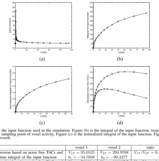
k13 = 0.0306, k14 = 0.0372 and k21 = 4.0716, k22 = 0.0387, k23 = 0.0507, k24 = 0.0229, respectively. The parameters are derived from a brain PET study of healthy control subjects using C-11 labeled DASB, as described in section V. The input function used in the simulation is shown in Figure 2(a), where the circles indicate the time points when the input function is sampled. Similar with the brain PET study in section V, the activity of the simulated voxels are measured at 18 serial time points, which are different from the sampling time points of the input function. Since our vector form formulation in equation (7) evaluates the integral of the input function at the time points that correspond to the measured voxel activity, we integrate the input function and resample it at the 18 time points of the voxel activity measurement, as shown in Figure 2(b). Moreover, in section III-A, it is mentioned that the activity-subspace approach is only able to estimate the direction of cint_p (the shape of the integral of the input function), and the estimated integral of the input function ˆcint_p is constrained to be a unit length vector. Therefore, a successful estimationˆcint_p will equal to the normalized integral of the input function, denoted as ¯cint_p = _|cint1

p |c

int

p . The normalized integral of the input function is shown in Figure 2(c), which is what we plan to estimate using the activity-subspace approach. The value of parameter t∗ is chosen to be t∗ = 20. In the simulated data and the real PET data, there are 6 time points after t∗ = 20. We choose t∗ to be as large as possible, while guaranteeing enough time points for

estimating the activity-subspaces and the integral of the input function.

Using the input function in Figure 2(a) and the kinetic parameters listed above, we simulate the TACs of the two voxels under the noise free case, shown in Figure 2(d). Base on the noise free TACs and the integral of the input function, the kinetic parameters in equation (6) can be obtained through linear regression. We also calculate the kinetic parameters based on the noise free TACs and the normalized integral of the input function. The results are shown in Table I. In this table, we can see that, the relative ratios between the two voxels’ distribution volumes in both cases are the same. In the case where normalized integral of the input function is used, the calculated distribution parameters of the two voxels are scaled by the same factor, compared with the case where the true integral of the input function is used. Therefore, for the purpose of estimating distribution volume para-metric image, the knowledge of the normalized integral of the input function will lead to the same performance with the case where the true integral of the input function is known. In the following, the normalized integral of the input function and the kinetic parameters in the bottom row of Table I will serve as the ground truth of the simulation.

In order to examine the impact of noise on the pro-posed activity-subspace approach, we consider a realistic noise model. As suggested in [18], the measurement error variance is proportional to the imaged radioactivity concentration and is inversely proportional to the scan duration. Therefore, we consider the noise model that noise terms are independent Gaussian with variances,

σ2(i, t_j) =αeλtjci(tj) tj−tj−1

, (17)

for j = 1, ..., n, where α is a constant determining the noise level; ci(tj) is the simulated noise-free TAC of voxel iat time tj; λis the radioisotope decay constant. Here, we define the percent noise level as

s P_n j=1σ 2_(i,t j) Pn j=1c 0 i(tj)2,

with {c0_i(tj)} being the noise-free TAC for voxel i. The noise levels ranging from 0% to 5% are tested in the simulation.

At each noise level, we simulate 1000 runs, generating 1000 pairs of noisy TACs of the two simulated voxels. In each run, the activity-subspace approach in section III-A is used to estimate the integral of the input function from the noisy TACs. With the estimated integral, the distribution volumes of the two simulated voxels are estimated by least square regression of equation (6). The ratio between the estimated distribution volumes is used to show the estimation performance. At each noise level,

0 20 40 60 80 100 −20 0 20 40 60 80 100 120 140 160 180 t (min) Input function 0 10 20 30 40 50 60 70 80 90 0 50 100 150 200 250 300 350 400 450 500 t (min)

Integral of input function

(a) (b) 0 10 20 30 40 50 60 70 80 90 0 0.1 0.2 0.3 0.4 0.5 0.6 0.7 t (min)

Normalized integral of input function

0 10 20 30 40 50 60 70 80 90 0 100 200 300 400 500 600 700 800 t (min)

Simulated noise−free TACs

(c) (d)

Fig. 2. Figure (a) is the input function used in the simulation. Figure (b) is the integral of the input function, resampled at the time points that correspond to the sampling point of voxel activity. Figure (c) is the normalized integral of the input function. Figure (d) shows the TACs of the two simulated voxels

voxel 1 voxel 2 ratio

regression based on noise free TACs and V1T= 95.0525 V2T = 294.9598 V1T/V2T = 0.3223

true integral of the input function b1=−34.5938 b2=−90.2277

regression based on noise free TACs and V1T= 72123.4 V2T = 223807.7 V1T/V2T = 0.3223

normalized integral of the input function b1=−34.5938 b2=−90.2277

TABLE I

KINETIC PARAMETERS OF SIMULATED VOXELS,CALCULATED BASED ON TWO CASES:NOISE FREETACS AND TRUE INTEGRAL OF THE

INPUT FUNCTION;NOISE FREETACS AND NORMALIZED INTEGRAL OF THE INPUT FUNCTION.

we calculate the average and standard deviation of the ratio from the 1000 simulation runs.

For the purpose of comparison, we implemented the Iterative Quadratic Maximum-Likelihood (IQML), be-cause IQML yields the best performance among the three blind estimation algorithms compared in [13]. There are both 2-compartment model and 3-compartment model versions of IQML [20]. Since the simulation is based on the 3-compartment model, due to the reason of no model mismatch, the 3-compartment model IQML yields more accurate result than that of the 2-compartment model one under noise-free case. However, the estimated distribution volume in 3-compartment IQML is very sensitive to noise even when very small noise is added and can be less accurate than that of the 2-compartment IQML. We think the intuitive reason is as follows. The 3-compartment model IQML does not directly estimate the distribution volume and it estimates a set of 4

parameters instead; the distribution volume is calculated via a complicated function of the estimated parameters and thus its estimation error can be severely amplified. Moreover, we believe that the comparison with the 2-compartment model IQML is more fair, because it has essentially the same complexity as the Logan plot in terms of the number of model parameters. Therefore, we choose to compare the proposed method with the 2-compartment model version of IQML. To ensure that IQML achieves its best performance, we use the true kinetic parameters as its initial. The results are shown in Table II.

In Table II, at the0%noise level, although the integral of the input function is estimated based on the noise free TACs, the estimation is not perfect. This is because of two reasons. First, the activity-subspace approach is based on the Logan plot, which is an asymptotically linear relationship for the later part of the TACs. Since

V1T/V2T Activity-subspace IQML

noise level mean std mean std

0 0.3236 0 0.2801 0 1 0.3247 0.0303 0.2799 0.0092 2 0.3334 0.0592 0.2780 0.0171 3 0.3502 0.0665 0.2759 0.0278 4 0.3675 0.0787 0.2729 0.0387 5 0.3921 0.0782 0.2741 0.0505 True ratioV1T/V2T= 0.3223 TABLE II

MEAN AND STANDARD DEVIATION OF THE RATIO BETWEEN THE

ESTIMATED DISTRIBUTION VOLUMES OF THE TWO SIMULATED

VOXELS.

the noise-free data is simulated based on the three-compartment model, there is model mismatch between the true three-compartment model and the Logan plot. Second, the activity-subspace of a voxel is spanned by the voxel TAC and its integral. With the 18 available time points of the voxel TAC, the numerical integration of the voxel TAC introduces error. For the same reason, IQML method also gives non-zero error at0%noise level. Since the IQML method assumes two-compartment model for the entire TAC, the model mismatch is larger, and thus a larger error is observed. At 0% noise level, since no noise is added, the estimation results from the 1000 runs are identical, which results in 0 standard deviation of the estimation error.

From Table II, we can see that the proposed activity-subspace is more sensitive to noise. This result is also confirmed in [15]. In this table, we can see that the IQML method, although more robust to noise, consistently generates biased estimates. This is again because of the model mismatch between the two-compartment model assumed by IQML and the three-compartment model based on which the data is simulated. On the other hand, the propose activity-subspace approach estimates the integral of the input function, which leads to more accurate estimates of the relative distribution volume. The only concern, so far, is the noise sensitivity.

Therefore, in order to obtain reliable estimates using the activity-subspace approach, the noise level needs to be kept small. This is our motivation for employing mPCA clustering. We also apply iterative least square method to further improve the accuracy of the estimated integral of the input function and simultaneously esti-mate the distribution volume parameters. In the following section, we analyze the data set from a brain PET study, and demonstrate that the activity-subspace approach, to-gether with the mPCA and iterative least square methods, is able to estimate both the integral of the input function and the distribution volume parametric image.

V. REALDATASETS

We now examine a brain PET study. The PET data of healthy control subjects is obtained after intravenous injection of C-11 labeled DASB, a radioligand used for imaging the serotonin transporter (SERT). The experi-mental details are the same as in [2]. In total, 10 subjects are tested . A dynamic PET study is performed with a GE Advance PET camera with an axial resolution (FWHM) of 5.8 mm, and an in plane resolution of 5.4 mm. This scanner acquires 35 simultaneous slices of 4.25 mm thickness. A transmission scan is first obtained with twin 10 mCi germanium-68 pin sources for 10 minutes for the purpose of attenuation correction of the emission scans. 18 serial dynamic PET images are acquired during the first 95 minutes after injection using the following image sequence: four 15 sec frames, three 1 min frames, three 2 min frames, three 5 min frames, three 10 min frames, and two 20 min frames. All PET scans are reconstructed using the Ramp-filtered back-projection technique in a 128x128 matrix, with a transaxial voxel size of 2x2 mm. All PET data are corrected for attenuation, injected dose and radionuclide decay.

For the invasive measurement of the input function, a radial artery line is placed by an anesthesiologist. During the PET study arterial blood samples are withdrawn every 5-7 seconds during the first two minutes, then with increasing time intervals until the end of study 95 minutes post injection. Exact times of blood sampling are registered. The blood samples are centrifuged and plasma activities are counted in a gamma counter cross-calibrated with the PET scanner every day. The exact time difference between the start of camera and the start of gamma counter is registered for decay correction. The input function is corrected for metabolized radioligand activity. For this purpose, 2 ml arterial plasma samples are obtained 5, 15, 30, 60 and 90 minutes post injection. The extent of metabolism of C-11 DASB is determined using high performance liquid chromatography (HPLC). Missing data points of the correction function that de-scribes the percent unmetabolized tracer are obtained by bi-exponential interpolation [2].

For the dynamic brain PET image data, we first perform preprocessing to identify voxels that belong to the brain region. A simple masking method is applied to sketch out the brain region. Based on the 18 dynamic PET images of the 18 time points, the sum of intensities of the observed TACs for all voxels are calculated. Vox-els with intensities less than 5%of the highest intensity voxel are regarded as non-scalp voxels and discarded. The remaining voxels are considered as the brain region for further estimation of the integral of the input function

0 10 20 30 40 50 60 70 80 90 0 0.1 0.2 0.3 0.4 0.5 0.6 0.7 t (min)

Integral of the input function

Normalized integral of measured input function Estimation from activity−subspaces Further Refinement by Iterative LS

(a) (b)

V

T image based on measured input function

20 40 60 80 100 120 20 40 60 80 100 120 0 0.5 1 1.5 2 2.5 x 105 V

T image based on estimated integral

20 40 60 80 100 120 20 40 60 80 100 120 0 0.5 1 1.5 2 2.5 x 105 (c) (d) Difference images 20 40 60 80 100 120 20 40 60 80 100 120 −4000 −2000 0 2000 4000 6000 (e)

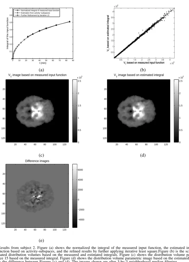
Fig. 3. Results from subject 2. Figure (a) shows the normalized the integral of the measured input function, the estimated integral of the input function based on activity-subspaces, and the refined results by further applying iterative least square.Figure (b) is the scatter plot of the estimated distribution volumes based on the measured and estimated integrals. Figure (c) shows the distribution volume parametric image of slice 15 based on the measured integral. Figure (d) shows the distribution volume parametric image based on the estimated integral. Figure (e) is the difference between Figures (c) and (d). The images shown are after 3-by-3 neighborhood median filtering.

and the distribution volume parametric image.

After preprocessing, the brain region is identified. In section IV, it is shown that, the proposed activity-subspace approach is sensitive to noise. Therefore, we cannot directly apply the activity-subspace approach based on the noisy voxel TACs. To reduce the noise, we take voxels from the brain regions of all slices, and apply the mPCA approach in section III-B to group the brain voxel TACs into two clusters. The activity of each cluster is represented by the average of voxel TACs within this cluster. Through averaging, the noise is reduced. Then, the integral of the input function is estimated using the activity-subspace approach, which operates on the cluster average TACs. In Figure 3(a), we use the data for subject 2 as an example. The estimated integral of the input function is shown by a solid line labeled with stars. The normalized integral of the measured input function is shown by the solid line labeled with circles. To improve the accuracy of the estimated integral of the input function, the iterative least square method in section III-C is applied to iteratively refine the estimated integral of the input function based on the TACs of all brain voxels. In Figure 3(a), the refined estimate of the integral is shown by the solid line labeled with triangles. After obtaining the estimated integral of the input function, we further estimate the relative distribution volumes. Based on the estimated integral of the input function, the relative distribution volume parameters are obtained by linear regression of equation (7) for each voxel [18]. For comparison, the relative distribution volume parameters are also calculated based on the normalized integral of the measured input function. In Figure 3(b), the scatter plot of the relative distribution volume parameters is shown, where each dot corre-sponds to one voxel, the horizontal and vertical axes represent the estimated parameters with the measured and estimated integral of the input function. The scatter plot closely follows the 45 degree line, which indicates high estimation accuracy. To quantify the estimation accuracy, we compute the normalized relative distance (PM) between the true and estimated parametric images. PM is defined to compare the two parametric images,

P M = 1 N N X i=1 |( ˆViT −V¯iT)/V¯iT|, (18)

whereV¯iT is the relative distribution volume obtained by the normalized integral of the measured input function,

ˆ

ViT is the estimated relative distribution volume based on the estimated integral of the input function, andN is the total number of voxels in the brain region. For subject 2, P M = 0.012, meaning that the distribution volume

subject P M subject P M 1 0.024 6 0.018 2 0.012 7 0.031 3 0.038 8 0.261 4 0.006 9 0.041 5 0.068 10 0.018 TABLE III

THEP MMETRIC THAT QUANTIFIES THE DIFFERENCE BETWEEN

THE DISTRIBUTION VOLUME PARAMETRIC IMAGE BASED ON THE PROPOSED METHOD AND THAT BASED ON THE MEASURED INPUT

FUNCTION.

image based on the estimated integral contain 1.2% error, compared with the distribution volume image based on the measured input function. In Figure 3 (c) and (d), we use slice 15 as example to show the distribution volume parametric images based on the measure and estimated integral of the input function. The difference image is shown in Figure 3(e). The images shown are after 3-by-3 neighborhood median filtering. In Figure 3 (c) and (d), both images show the expected high binding in the region of basal ganglia and the midbrain.

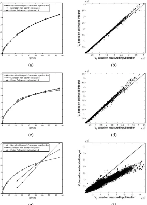
In total, we analyze 10 subjects. In Table III, we show the P M that quantifies the difference between the distribution volume parametric images based on the estimated and measured integrals of the input function. From Table III, theP M error for most of the subjects are small, and the average P M is 5.2%. Excluding subject 8 with extremely largeP M, the average error reduces to 2.8%. To better illustrate the estimation error, in Figure 4, we show the estimated integral and the scatter plot of estimated distribution volumes, (a) and (b) for subject 1, whoseP Mis 2.4%; (c) and (d) for subject 9, whoseP M

is 4.1%; (e) and (f) for subject 8, whose P M is 26.1%. For subject 8, the proposed method gives an incorrect estimate of the integral. The scatter plot in Figure 4 (f) shows a linear relationship. The estimated distribution volume image is of lower contract, compared with the case where the input function is measured. Therefore, the estimated distribution volume image is qualitatively meaningful but quantitatively incorrect. For the other nine subjects, the proposed method is able to estimate the integral of the input function and the distribution volume parametric image, giving an average error of 2.8.%.

VI. DISCUSSIONS

In this paper, we presented an activity-subspace ap-proach for estimating the integrated input function and the relative distribution volume parametric image. Rather than providing absolute quantification, the proposed method only estimates the relative distribution volume

0 10 20 30 40 50 60 70 80 90 0 0.1 0.2 0.3 0.4 0.5 0.6 0.7 t (min)

Integral of the input function

Normalized integral of measured input function Estimation from activity−subspaces Further Refinement by Iterative LS

(a) (b) 0 10 20 30 40 50 60 70 80 90 0 0.1 0.2 0.3 0.4 0.5 0.6 0.7 t (min)

Integral of the input function

Normalized integral of measured input function Estimation from activity−subspaces Further Refinement by Iterative LS

(c) (d) 0 10 20 30 40 50 60 70 80 90 0 0.1 0.2 0.3 0.4 0.5 0.6 0.7 t (min)

Integral of the input function

Normalized integral of measured input function Estimation from activity−subspaces Further Refinement by Iterative LS

(e) (f)

Fig. 4. The left column is the measured and estimated integrals of the input function. The right column is the scatter plots of the estimated distribution volume parameters. Figure (a) (b) correspond to subject 1; (c) (d) correspond to 9; (e) (f) correspond to subject 8.

within a scale factor. The scale factor is a common issue to any blind identification methods where no assump-tions are made on the unknown input function. When analyzing PET data of a single subject, the relative distri-bution volume is useful for comparisons across different slices or ROIs. For comparisons across subjects, an im-portant issue, absolute quantification of the distribution volume, needs to be addressed, and therefore additional assumptions or additional data are required. For example, if the total amount of dosage is controlled such that the integrals of the input functions of different subjects are the same, the proposed method can be applied. If the

artery is included in the dynamic images, after metabolite correction, the ratio between the input functions of two subjects can be inferred from the intensities of the artery voxels, and we can further use the ratio to adjust the estimated relative distribution volumes of the two subjects. Another possible option for achieving absolute quantification is to take a single arterial sample during scanning (or a venous sample if the relationship between arterial concentration and venous concentration is well established) to provide a reasonable estimate of the scale factor, though more research efforts may be needed for determining the optimal time point to take the sample.

In the analysis of the PET DASB study in Section V, the measured input function is considered as the

gold standard. [4] shed light on the validity of this gold standard. In [4], it was shown that the estimated

kinetic parameters by several methods were consistent, including the Logan plot [17] and a reference tissue method SRTM [9]. Logan plot assumed knowing the measured input function, while SRTM assumed a ref-erence region. Although the two methods started from different assumptions, the estimated kinetic parameters were consistent, indicating that both the measured input function and the reference region were correct. In Section V, we observe that, in most subjects, the estimated integral of the input function is close to the normalized integral of the measured input function. This observation enhanced our belief that, it is reasonable to regard the measured input as the gold standard in this study.

A challenging question general to blind identification methods is that how to tell whether the estimates are correct or not, when the true parameters are unknown. We are lack of a theoretical answer to this question. Heuristically, it is observed from Figure 4(e) that the estimated integral of the input function is incorrect since the shape of the integral is clearly incorrect. For more challenging cases where the shape of the estimated inte-gral may look correct, though not observed in our study, one possible solution is to examine the statistical stability via bootstrap, similar to the reproducibility idea in [4]. We can generate bootstrapped data sets and estimate the integral from each bootstrapped data set. If the estimated integrals from different bootstrapped data are statistically consistent, we can have certain confidence in the result; if otherwise, this can be an indication of failure.

VII. CONCLUSION

Of interest in this paper is the estimation of the total distribution volume parametric image in PET study when the knowledge of the plasma input function is not available. In this paper, we have presented a novel concept of activity-subspace, and derived the method for estimating the integral of the input function by exploring the intersections of the activity-subspaces spanned by the voxel cluster TACs and their integrals. No prior information regarding the input function or the reference region is needed in the proposed method. We presented the mixture Principal Component Analysis to group the brain voxels into clusters, so that the noise is reduced and the activity-subspace approach is able to estimate the integral of the input function more reliably. An iterative least square method is incorporated to further improve the accuracy of the estimated integral of the input function. Results from a PET brain study show that, for

the noninvasive studies when the measurement of plasma input function or a reference region is unavailable, the proposed activity-subspace approach, together with the mPCA method and the iterative least square method, is able to efficiently estimate the integral of the input function and the distribution volume parametric images. In a real dynamic PET data set of 10 subjects, the proposed method achieved an average error of 5.2% compared with the case where the true input function is measured and known.

APPENDIX

An EM algorithm for estimating mPCA model is proposed in [19]. The algorithm can be summarized as follows. Given the model parameters from initialization or previous iteration, the probability of observation yi conditioning on thekthprobabilistic PCA model param-eters can be calculated,

p(yi|k) = R p(yi|x, k)p(x|k)dx = (2π)−d/2_|C k|−1/2e− 1 2(yi−µk) T_C−1 k (yi−µk) (19) whereCk=σ2kI+WkWkT. Given the prior probabilities

p(k) of a set of K probabilistic PCA models, the marginal probability of observationyi is,

p(yi) = K

X

k=1

p(yi|k)p(k), (20) and the posterior probability of thekthprobabilistic PCA model can be expressed as

p(k|yi) = p(y_pi|₍i_y)p(k)

i) . (21)

Therefore, the posterior probability can be used for the classification purpose.

In the M-step, the update of model parameters can be summarized as follows. Suppose there are in total N

voxels under consideration.

e p(k) = 1 N N X i=1 p(k|yi) e µk = P_N i=1p(k|yi)yi P_N i=1p(k|yi) f Wk = SkWk(σ2kI+Mk−1WkTSkWk)−1 e σ2_k = 1 dtr(Sk−SkWkM −1 k WfkT)

where,pe(k),µek,Wfk,σe2_kare the updated model parame-ters for thekth probabilistic PCA model in the mixture, and S_k = 1 e p(k)N N X i=1 p(k|yi)(yi−µek)(yi−µek)T Mk = σ2kI +WkTWk

REFERENCES

[1] S.R. Cherry, “Fundamentals of Positron Emission Tomography and Applications in Preclinical Drug Development”, Journal of

Clinical Pharmacology, vol. 41, pp. 482-491, 2001.

[2] L. Kerenyi, G.A. Ricaurte, D.J. Schretlen, U. McCann, J. Varga, W.B. Mathews, H.T. Ravert, R.F. Dannals, J. Hilton, D.F. Wong, and Z. Szabo, “Positron Emission Tomography of Striatal Serotonin Transporters in Parkinson’s Disease”, Arch

Neurol, vol. 60, pp. 1223-1229, 2003.

[3] R.N. Gunn, S.R. Gunn, and V.J. Cunningham, “Positron Emis-sion Tomography Compartmental Models”, Journal of Cerebral

Blood Flow and Metabolism, vol. 21, no. 6, pp. 635-652, 2001.

[4] W.G. Frankle, M. Slifstein, R.N. Gunn, Y. Huang, D.R. Hwang, E.A. Darr, R. Narendran, A. Abi-Dargham, and M. Laruelle, “Estimation of Serotonin Transporter Parameters with 11C-DASB in Healthy Humans: Reproducibility and Comparison of Methods”, J Nucl Med., vol. 47, pp. 815-826, 2006. [5] V.J. Cunningham and A.A. Lammertsma, “Radioligand Studies

in Brain: Kinetic Analysis of PET Data”, Med. Chem. Res, vol. 5, pp. 79-96, 1994.

[6] J.H. Meyer and M. Ichise, “Modeling of Receptor Ligand Data in PET and SPECT Imaging: A Review of Major Approaches”,

Journal of Neuroimaging, vol. 11, no. 1, pp. 30-39, 2001.

[7] J. Correia, “Editorial: A Bloody Future for Clinical PET”,

Journal of Nucl. Med., vol. 33, pp. 620-622, 1992.

[8] K. Chen, D. Bandy, E. Reiman, S.C. Huang, M. Lawson, D. Feng, L.S. Yun, and A. Palant, “Noninvasive quantification of the cerebral metabolic rate for glucose using positron emission tomography,18F-fluoro-2-deoxyglucose, the patlak method, and an image-derived input function”, J. Cereb. Blood Flow Metab., vol. 18, pp. 716723, 1998.

[9] A.A. Lammertsma and S.P. Hume, “Simplified Reference Tissue Model for PET Receptor Studies”, Neuroimage, vol. 4, no. 3, pp. 153-158, 1996.

[10] R.N. Gunn, A.A. Lammertsma, S.P. Hume, and V.J. Cunning-ham, “Parametric Imaging of Ligand-Receptor Binding in PET Using A Simplified Reference Region Model”, Neuroimage, vol. 6, no. 4, pp. 279-287, 1997.

[11] K.P. Wong, D. Feng, S.R. Meikle, and M.J. Fulham, “Si-multaneous Estimation of Physiological Parameters and Input Function - In vivo PET Data”, IEEE Trans. Inform. Tech.

Biomed., vol. 5, pp. 67-76, 2001.

[12] Z.J. Wang, Z. Szabo, P. Lei, J. Varga, and K.J.R. Liu, “A Factor-Image Framework to Quantification of Brain Receptor Dynamic PET Studies”, IEEE Trans. on Signal Processing, special issue

on Signal Processing Aspects of Brain Imaging, vol. 53, no. 9,

pp.. 3473-3487, 2005.

[13] D.Y. Riabkov and E. Di Bella, “Estimation of Kinetic Param-eters Without Input Functions: Analysis of Three Methods for Multichannel Blind Identification”, IEEE Trans. on Biomedical

Eng., vol. 49, no. 11, Nov. 2002.

[14] Z.J. Wang, P. Qiu, K.J.R. Liu, and Z. Szabo, “Model-Based Receptor Quantization Analysis for PET Parametric Imaging”,

IEEE Engineering in Medicine and Biology Conference, pp.

5908-5911, 2005.

[15] M. Naganawa, Y. Kimura, J. Yano, M. Mishina, M. Yanagisawa, K. Ishii, K. Oda, and K. Ishiwata, “Robust Estimation of the Arterial Input Function for Logan Plots using an Intersectional Searching Algorithm and Clustering in Positron Emission To-mography for Neuroreceptor Imaging”, NeuroImage, vol. 40, no. 1, pp. 26-34, 2008.

[16] P. Qiu, Z.J. Wang, and K.J.R. Liu, ”Mixture Principal Com-ponent Analysis for Distribution Volumn Parametric Imaging in Brain PET Studies”, IEEE International Symposium on Biomedical Imaging (ISBI), pp. 928-931, 2006.

[17] J. Logan, J.S. Fowler, N.D. Volkow, A.P. Wolf, S.L. Dewey, D.J. Schlyer, R.R. MacGregor, R. Hitzeman, B. Bendiriem, S.J. Gatley, and D. Cristman, “Graphical Analysis of Reversible Radioligand Binding from Time-Activity Measurements Ap-plied to[N−11_C−

methyl]-(-)-cocaine PET Studies in Human Subjects”, J. Cereb Blood Flow Metab, vol. 10, pp. 740-747, 1990.

[18] M. Ichise, H. Toyama, R.B. Innis, and R.E. Carson, “Strategies to Improve Neuroreceptor Parameter Estimation by Linear Regression Analysis”, Journal of Cerebral Blood Flow &

Metabolism, vol. 22, pp. 1271-1281, 2002.

[19] M.E. Tipping and C.M. Bishop, “Mixtures of probabilistic prin-cipal component analyzers”, Neural Computation, 11(2):443-482, 1999.

[20] D.Y. Riabkov and E. Di Bella, “Blind identification of the kinetic parameters in three-compartment models”, Phys. Med.