A Numerical and Experimental Investigation of Flow
Separation Control over a Wall-Mounted Hump Model
Mehti Koklu 1
NASA Langley Research Center, Hampton, VA 23681
Numerical simulations and wind tunnel experiments were performed to investigate flow separation and its control over a wall-mounted hump model. Three-dimensional, unsteady fluid dynamic simulations were used to capture the relevant flow physics of unsteady flow separation and its control via active and passive flow control methods. Surface pressure measurements and surface oilflow visualization were obtained in the experiments. Current measurements documented a considerably thinner incoming boundary layer, but similar pressure distribution, compared to the reference data reported in the CFD Validation (CFDVAL 2004) Experiments. Consistent with the data available in the literature, numerical simulations predicted a longer separation bubble, which manifested itself as a shift in the pressure distributions. Streamwise vortices generated by passive vortex generators increased the suction pressure and provided substantial pressure recovery. Numerical simulations of vortex generators qualitatively predicted the effects of control, and revealed patterns of attached/separated flow regions. On the other hand, active flow control using steady discrete jets reduced, but was not able to eliminate, flow separation for the tested configuration. Although the major disagreement between the numerical and experimental results was in the pressure recovery region due to the inaccurate prediction of separation bubble, the relative pressure recoveries from the baselines were comparable. Surface oilflow visualization and simulated surface streamlines were qualitatively in good agreement revealing the key flow features.
Nomenclature
c = hump chord
Cp = pressure coefficient
Cf = skin friction coefficient
λ2 = second eigenvalue of the velocity gradient tensor
Rec = Reynolds number based on hump chord
tc = characteristic time
U = freestream velocity
V = velocity magnitude
x,y,z = streamwise, vertical, spanwise directions
I.
Introduction
Flow separation is a phenomenon encountered in many engineering applications and developing methods to control flow separation has immense importance as it could help improve the performance of fluidic machinery. Various active and passive flow control concepts have been proposed to control flow separation with varying degrees of success. Performance assessment of these flow control concepts is even challenging when considering the multitude of experimental models being used. A wall-mounted hump model is a perfect candidate to investigate different flow separation control techniques, as it is a well-known benchmarking case for computational fluid dynamic (CFD) validations. The key advantage of the wall mounted hump model is that the model was shown to have negligible sensitivity to Reynolds number and the incoming boundary layer.1-3 This is particularly important because it allows scaling of the wind tunnel results. Another key advantage is the sensitivity of separated flow to a flow control mechanism. The nature of the separated flow over the hump model makes it more responsive to flow control such
2
that the effects of flow control are more evident. The model was one of the case studies in the CFD Validation of Synthetic Jets and Turbulent Separation Control Workshop (CFDVAL2004) in 2004 and is well documented both experimentally2-5 and numerically6 over a wide range of Reynolds numbers (0.4 x 10⁶ < Re
c< 26 x 106). Zero net mass flow actuators,4 steady suction,1-3 unsteady blowing,3 and fluidic oscillators7-8 were previously used to control flow separation over the hump model.
In this study, both passive (vortex generators) and active (steady blowing) flow control methods were used to control flow separation. These methods have been used to control flow separation on different models in the past; however, in this study the numerical simulations and wind tunnel experiments were carried out in parallel in order to understand the effect of these flow control techniques on flow separation over a well-known model. The accurate prediction of massively separated flows (e.g., flow over the hump) is still challenging but the CFD simulations provide key contributions in understanding mechanisms associated with flow separation and its control with different flow control techniques. Although this model has been used as a turbulence model validation case by CFD researchers, it should be noted that this study is not a code development/validation study but a computational and experimental study that aims to better understand the effect of active and passive flow control methods on separated flow.
II.
Experimental & Computational Setup
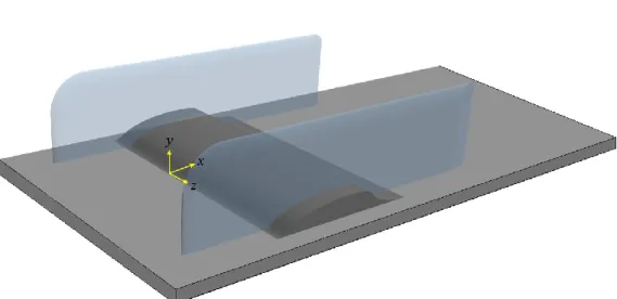
The model used in this study is a wall-mounted hump model, which is the suction side of a Glauert-Glass II airfoil that was originally designed by Glauert.1 The wall-mounted hump model was previously tested in low2,4 and high3 Reynolds number flows. It is the same model that was used by Greenblatt et al.2,4 during the CFDVAL2004 Workshop in 2004. Experimental data reported in the workshop will be used as a reference to compare the current results. The details about the model and the wind tunnel conditions can be found in Ref. [2]. Only a brief summary will be given here. The CAD rendering of the hump model is shown in Fig. 1. The characteristic length is defined as the hump chord (c), which is 420 mm. The original model had a two dimensional slot located at x/c = 0.65 that was connected to an interior plenum spanning the entire model width (584 mm) between the forebody and ramp. The model mid-section, which included the slot, was refabricated to accommodate an array of flow control actuators (i.e., jet nozzles). The experiments were conducted in the NASA Langley 20 x 28 in. wind tunnel at a freestream Mach number of 0.1, which corresponded to Rec = 0.94 x 10⁶ based on the hump chord. The experimental configuration was chosen to match that of Ref. [2] for comparison. The model was mounted on a splitter plate and between two endplates. The boundary layer was tripped near the leading edge of the splitter plate using 20 mm thick (#60) sand paper.
Surface static pressure measurements are reported in this study. The model has 124 static pressure ports (0.5 mm orifice diameter) along the centerline. There are two arrays of spanwise pressure ports on the forebody (x/c = 0.19) and on the ramp (x/c = 0.86) sections to check the flow uniformity before and after flow separation. The static pressure ports were connected to electronically scanned pressure modules and time averaged static data was recorded at each pressure port. Oilflow visualization was performed to map the surface flow patterns. The surface flow visualization was obtained using a mixture of kerosene, aviation oil, and fumed silica particles. Details of the flow visualization technique can be found in Ref. [9]. The mixture was applied to black contact paper mounted on the hump model and was moved under the effect of local shear stresses. Fluorescent pigment in the aviation oil glows under UV lighting and reveals the surface flow patterns.
The unsteady numerical simulations presented in this paper were performed using a commercial software package, which is a compressible flow solver based on Lattice Boltzmann Model (LBM).10 The model solves the three-dimensional, unsteady lattice Boltzmann equation in conjunction with hybrid turbulence modeling that involves very large eddy simulation approach. The hybrid turbulence modeling approach directly resolves large, energy-containing scales, whereas the smaller scales are modeled using modified k−ϵ turbulence model. In addition, appropriate wall functions11 were utilized to capture the boundary layer behavior without excessive grid resolution near the solid walls. The LBM equation was solved on embedded Cartesian meshes (voxels), which were generated automatically within the flow solver. Local mesh refinements were performed near high gradient regions (e.g., shear layers) using variable resolution regions (Fig. 2). The model uses an explicit time advancement scheme, which allows massively parallel simulations.
The computational modeling included the three-dimensional hump geometry, endplates, and splitter plate. The length of the splitter plate upstream of the model was similar to the experiment (4.6c) in contrast to the previous simulations that lengthened the splitter plate (6.4c) in order to match the boundary layer profile at the inflow location (x/c = -2.14). In the simulations, a viscous no-slip boundary condition was imposed on solid walls, whereas the tunnel sidewalls and ceiling were treated as inviscid walls to eliminate the additional cost of resolving boundary layers. A constant velocity (Mach number of0.1) inlet and atmospheric pressure outlet boundary conditions were prescribed at
the inflow and outflow, respectively. For the active flow control case, a constant mass flow boundary condition (0.003 kg/s) was used at the nozzle inlets to generate steady discrete jets.
As a first step in the numerical simulations, a mesh dependence study was performed to confirm that the obtained solutions were independent of the grid resolution. For this purpose, the baseline-separated flow was simulated at four different (coarse, medium, fine, finest) grid resolutions that have 17, 27, 53, 92 million fine equivalent voxels, respectively. The fine and finest grid resolutions provided relatively close results; therefore, it is anticipated that at least a fine grid resolution with 53 million fine equivalent voxels is required to provide a grid independent solution. The smallest voxel size for the fine grid resolution was 0.4 mm. The physical time step was automatically adjusted depending on the finest voxel size (i.e., Δt = 6.87 x 10⁻⁷ s in this case). The simulations were carried out 10 characteristic times (tc = c/U). The state of simulations was monitored using the variables recorded at the probe locations at very high frequency. Since the solutions were initialized from rest, the data for the first 3tc were discarded in order to remove the effects of the initial transient phase. Remaining solutions were divided into ten frames (each averaged over 0.7tc) to provide unsteady data. Time averaged data was then obtained by averaging these ten frames.
III.
Results
A. Baseline Separated Flow
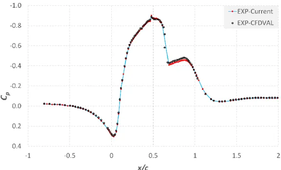
The boundary layer characteristics of the incoming flow to the hump model will be reported first. The boundary layer profile at the inflow (x/c = -2.14) location was measured using a hotwire anemometer and compared to that of the reference data (i.e., CFDVAL2004 experiments) in Fig. 3. As shown in this figure, the current boundary layer is considerably thinner than the reported boundary layer data (19 mm vs. 30.5 mm). Similarly, the current momentum thickness is almost 50% less (2.14 mm vs. 3.11mm) than the previously reported data. The reason behind this discrepancy in the incoming boundary layer was attributed to a possible separation bubble at the leading edge of the splitter plate due to the suction manifold used in the CFDVAL2004 experiments.2 The figure also presents the boundary layer profile obtained by the current numerical simulations for the baseline case. As shown, the simulated boundary layer profile is in good agreement with the current boundary layer measurements. This is expected because the length of the splitter plate was the same for both the current experiment and numerical simulation; whereas, the researchers had to extend the splitter plate farther upstream (to -6.4c) to match the incoming boundary layer profile at the inflow location in the CFDVAL workshop. Although the incoming boundary layers were different in the two experiments, this model was shown to be negligibly sensitive to the incoming flow.3 This is presented in Fig. 4, where the centerline pressure (Cp) distribution is compared to that of the reference dataset. Overall, the current Cp distribution agrees very well with the reference dataset. Flow deceleration (x/c < 0), flow acceleration (0 < x/c < 0.5), suction peak (x/c ≈ 0.5), and flow separation at x/c ≈ 0.66 (indicated by a plateau in the Cp distribution) are all in good agreement with the reference dataset with the exception of the flow reacceleration region (0.67 < x/c < 0.93) where the current measurements are slightly offset. After the flow reacceleration region, the current pressure measurements again provided a similar Cp distribution to the reported dataset. This minor offset in the Cp distribution inside the separation bubble might be due to the difference in the incoming boundary layer and/or slight variation in the tunnel configurations.
Figure 5 compares the numerical results to the experimental results for the baseline case. Since the LBM is by definition an unsteady flow solver, the Cp distribution also presents error bars that define the range of the pressure data at the particular locations. As shown in this figure, the error bars are quite large especially in the pressure recovery region. While the simulated centerline pressures are within 1% of the mean pressure distribution upstream of flow separation, it deviates as high as 5% near the flow reattachment region due to the intermittent nature of flow reattachment. Numerical results agree well with the experimental results up to the flow separation location. The simulation also captured the level and location of the flow reacceleration due to the separation bubble but could not accurately predict the size of the separation bubble. The second peak in the Cp distribution due to the separation bubble is near x/c = 0.89 for the experiment whereas, it is approximately at the model trailing edge (x/c = 1) for the simulation. The trend of the pressure recovery is also similar but due to the larger separation bubble, the pressure recovery curve is shifted in the streamwise direction.
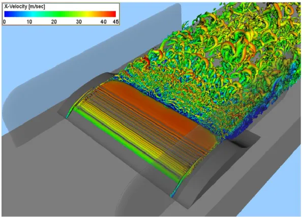
An illustration of the three-dimensional turbulent structures generated by flow separation is presented in Fig. 6. In this figure, instantaneous iso-surfaces of 2 – criterion were colored by the streamwise velocity to highlight the vortex cores. As shown in this figure, there is a thin attached shear layer over the hump model until the flow separation location. Then the shear layer separates and sheds from the hump surface resulting in formation of a wide variety of three-dimensional turbulent structures. These vortical structures convect and eventually diffuse downstream (not
4
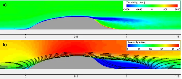
centerline (Fig.7a). Consistent with the Cp distributions in Figs. 4-5, the shear layer separates near x/c = 0.66 similar to the experiment and diffuses downstream. Figure 7b shows the contours of streamwise velocity at the centerline. Flow deceleration at the leading edge and flow acceleration over the hump model until flow separation (x/c = 0.66) can be seen in this figure. The streamlines reveal the predicted extent of the separation bubble.
The comparison of the computed and previously measured skin friction coefficient, Cf, is given in Fig. 8. In general, we see similar trends but not perfect agreement. In the flow deceleration region and x/c < 0.1 regions, the simulations agree well with the experiments but overpredict the skin friction coefficient in the favorable pressure gradient region (0.1 < x/c < 0.5). Skin friction prediction in the favorable gradient region was problematic for most of the computational methods (Large Eddy Simulation,12 Implicit Large Eddy Simulation and Reynolds Averaged Navier-Stokes Simulations,13 Lattice Boltzmann Method,14and see Ref [15] for other CFD methods) that computed the reference case, predicting considerably higher skin friction coefficient. There are Cf anomalies near x/c = -0.1, 0.45, 0.9, and, 1.1. Although the reason for these anomalies is not known, they are found to be at the juncture of different variable resolution regions. At these locations, the voxel size doubles; therefore, there might be a discontinuity in the velocity gradient due to the voxel size change. This might cause a sudden variation in the skin friction value but it quickly recovers to local skin friction values. Similar anomalies were also reported in the numerical simulation of Duda et al.16 Slightly upstream and downstream of the flow separation, numerical results are again in good agreement with the experiment. Therefore, the flow just prior to separation has similar shear stress values to the experiment. As mentioned before, the numerical simulation predicted a longer separation bubble. Flow reattachment is found to be at x/c = 1.266, indicating an almost 15% longer separation bubble compared to the reference data (x/c = 1.1). This resulted in a Cf distribution that is shifted in the streamwise direction with a similar trend and magnitude compared to that of the experiment.
Figure 9 shows the time-averaged streamwise velocity profiles at different stations (shown by dashed lines) at the centerline and compares them to the experimental data given in the reference dataset.2 Although close, the boundary layer just prior to flow separation (at x/c = 0.65) appears to be slightly thicker in the simulations. This implies that although the wall shear stresses were over predicted in the favorable pressure gradient region, the attached flow just prior to flow separation was predicted well with a correct momentum. The slightly higher momentum boundary layer carried over to downstream locations where the simulations consistently predicted thicker boundary layers with more momentum deficit. This resulted in a larger separation bubble compared to the experiment. The CFDVAL2004 experiment reported the flow reattachment as x/c = 1.1 where the simulations still show reverse flow and it is not until
x/c = 1.3 that positive surface flow velocities are observed. The magnitude of the reverse flow near the hump surface appears to be similar inside the separation bubble (at x/c = 0.8, 0.9, 1) as is consistent with the close surface skin friction values in Fig. 8.
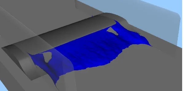
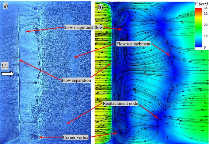
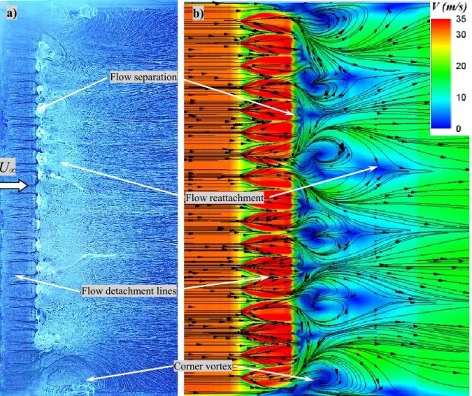
The three-dimensional extent of separation bubble over the hump model between two endplates is illustrated in the iso-surfaces of x-velocity = 0 in Fig. 10. The separation bubble is symmetric about the centerline and the signature of the corner vortices (x-velocity > 0) and its effect on the separation bubble are seen in this figure. Due to the corner vortices, shorter separation bubbles are observed near the endplates on each side and a relatively longer separation bubble is observed in between, especially near the centerline. A better demonstration of the separation bubble can be presented using surface flow visualization. Experimental and numerical surface flow visualizations of the separated flow between two endplates are presented in Fig. 11a and Fig. 11b, respectively. In these figures, the tunnel flow direction is from left to right. The surface flow visualization was obtained by oilflow visualization (Fig.11a) in the experiment whereas the numerical simulations used the near surface streamlines to visualize the surface flow (Fig. 11b). Contours in Fig.11b represent the velocity magnitude (V), which is minimum near the flow separation and reattachment regions. The minimal velocity magnitude (i.e., minimal shear stress) agrees with the negligible oil movement in the surface oilflow visualization in Fig. 11a. Key flow features (flow separation, flow reattachment, reattachment nodes, and corner vortices) are shown side by side in both figures. Visually, the corner vortices in the simulation appear to be larger than that of the oilflow visualization from the experiment. This is expected because it is known that the current turbulence models are incapable of accurately predicting the corner vortices.17 Flow separation appears to be two-dimensional and is located at x/c = 0.66 for both the experiment and simulation. The reattachment location near the centerline is found to be at x/c = 1.15 in the experiment (from oilflow visualization) and moves upstream to x/c = 1.11 near the endplates. The larger corner vortices in the simulation caused a less eccentric reattachment line, resulting in a longer separation bubble near the centerline and shorter separation bubbles near the endplates compared to the experiment. In the simulation, the reattachment location is x/c = 1.266 near the centerline and x/c = 1.12 downstream of the corner vortices. This is more than a 12% deviation in the reattachment location across the model span.
B. Flow Control with VGs
The first method studied in controlling flow separation on the hump model is vortex generators (VGs). VGs are passive flow control devices that increase the boundary-layer mixing through the generated streamwise vortices 18 This in turn energizes the near-wall fluid momentum and enhances its resistance to adverse pressure gradient. VGs were made out of 5 mm high and 19 mm long thin-metal shim stock in a right trapezoidal shape (Fig. 12 inset). Seventeen counter rotating (or diverging) VG pairs were installed laterally across the span. The spacing between the diverging-VG pairs was 33 mm and the center-VG pair (ninth pair) was located at the model centerline. The leading edges of the VGs were 3 mm away from VG symmetry line. VGs were installed near the suction peak (x/c = 0.48) in the streamwise direction and oriented at ±23 degrees with respect to the freestream direction to generate stronger streamwise vortices (Fig. 12).18 Diverging-VG pairs generate counter rotating vortices that induce downwash flow in between. On the other hand, converging-VG pairs (Fig. 12 inset) also generate counter rotating vortices but induce upwash flow in between.
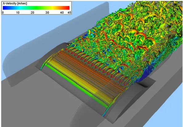
Flow separation control with a similar VG configuration was previously reported in Ref [8]. In that study, the centerline pressure ports between the center-VG pair were blocked by the VG array. In this study, the VG flow control case was repeated without blocking the pressure ports between the center-VG pair in order to compare to the numerical simulations. A perspective view of the instantaneous flow field is shown by the iso-surfaces of 2 –criterion that were colored by the streamwise velocity in Fig. 13. Streamwise vortices generated by VGs are clearly shown in the figure. These streamwise vortices convect downstream and interact with the shear layer to form different scaled three dimensional flow structures. Downstream of the VGs, streamwise vortex pairs generated by diverging VGs appear to depart from each other; in another words, the vortex pairs generated by converging-VGs converge before reaching the adverse pressure gradient.
Figure 14 presents the simulated centerline Cp distribution of the VG flow control case and compares it to the experimental data. The figure also includes the simulated Cp distributions for the baseline and the VG flow control cases at the centerline and off-center, respectively. All of the Cp distributions are in good agreement until the model mid-chord. There is an impulsive jump in the centerline Cp distribution that starts approximately at x/c = 0.48 (leading edge of the VGs) and peaks at x/c = 0.5 (upper left corner of VGs). This is because the tunnel centerline is affected by the counter rotating vortex pair that induces downwash flow. The downwash flow brings high momentum flow from outside the boundary layer to the near wall and hence increases the near wall fluid momentum. This local acceleration peaks at x/c = 0.5 due to the triangular part of the VGs as it generates a growing vortex pair. As shown in this figure, this local jump in the suction pressure is well predicted by the numerical simulations. The peak suction pressure in the simulation is lower than the experiments possibly due to the imperfect alignment of VGs in the experiment. After the peak, the pressure immediately recovers to the local tunnel flow pressures approximately at the trailing edge of the VGs. On the other hand, the off-center Cp distribution (between the converging-VG pair) shows first a dip at x/c = 0.5 and then recovers to the local tunnel flow pressures due to the induced upwash flow that increases the boundary layer thickness locally. There is another peak in the experimental Cp distribution near x/c = 0.61 possibly due to the limited number of pressure ports between x/c = 0.5 and x/c = 0.68. As shown in this figure, the simulated centerline Cp distribution shows similar trends and the suction pressure increases up to the crest of the flow separation location (x/c = 0.65). This second peak is not observed in the off-center (converging-VG pair) Cp distribution; instead, the pressure starts to recover immediately downstream of the VG trailing edges. After the nominally separated flow region, x/c = 0.66, there is a steep pressure recovery at the centerline. It is not possible to determine the existence of a separation bubble by looking at the centerline Cp distributions, as the pressure smoothly recovers. However, the off-center Cp distribution shows a plateau downstream of converging-VGs, which indicates a separation bubble. In fact, the Cp distribution is higher than the baseline case, which implies that the VGs promoted flow separation locally at this region. This figure clearly shows that even though flow separation is promoted downstream of converging-VGs, the application of VGs provided substantial pressure recovery compared to the baseline.
Spanwise vorticity contours at the centerline (Fig. 15a) and off-center plane (Fig. 15b) assist in explaining the different Cp distributions in the previous figure (Fig. 14). The all negative near wall vorticity distribution in Fig.15a suggests an attached flow at the centerline. The near wall vorticity downstream of the VGs is slightly thinner compared to the upstream locations as well as to the baseline case (Fig. 7a), which confirms flow acceleration that was shown in the Cp distribution. On the other hand, the off-center near wall vorticity (Fig. 15b) is slightly thicker downstream of VGs and flow separation is promoted as shown by the shear layer being separated early. The separated shear layer appears to be shorter than that of the baseline case indicating a shorter separation bubble. The positive near wall vorticity immediately downstream of flow separation is higher than that of the baseline case indicating a higher circulation level of the separation bubble.
6
Figure 16 presents the simulated velocity profiles of VG flow control and the baseline cases at different streamwise locations similar to that shown in Fig. 9. Prior to flow separation (at x/c = 0.65), the boundary layer of the VG flow control case is much fuller than the baseline case due to the generated streamwise vortices that energized the boundary layer. The higher momentum boundary layer resists the adverse pressure gradient and as shown at x/c = 0.8, the velocity profile does not show any reverse flow at this particular location (i.e., centerline). Although the boundary layer momentum gradually reduces downstream due to adverse pressure gradient, none of the velocity profiles show any sign of flow separation at downstream locations.
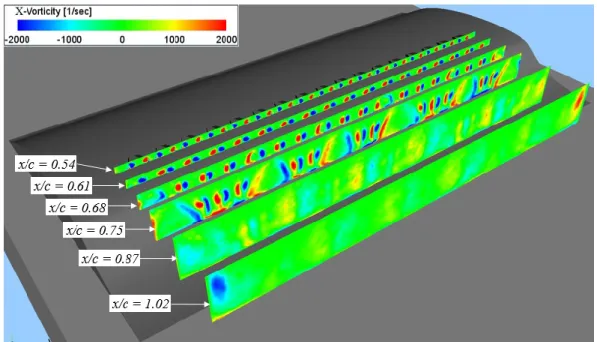
The previous figures (Figs. 14-16) showed the effect of generated vortices at the spanwise planes (i.e., centerline and off-centerline). The streamwise vorticity contours at different streamwise planes (x/c = 0.54, 0.61, 0.68, 0.75, 0.87 and 1.02) in Fig. 17 give insight about how the generated vortices evolve and convect downstream. The endplates were set to invisible in order not to block the view. The streamwise vortices generated by each VG are seen immediately downstream of the VG trailing edges (x/c = 0.54). These streamwise vortices are evenly distributed in the spanwise direction. Farther downstream, at x/c = 0.61 and 0.68, the upwash vortex pairs (generated by converging VGs) get closer. The streamwise vortices are observed to be stretched in the vertical direction (x/c = 0.68) and the stretching is not identical for all; hence, some of the vortex pairs are no longer symmetric. These asymmetric vortex pairs appear to depart from each other at x/c = 0.75 forming a gap in between. There are four detached vortex pairs (or gaps) in the domain. The streamwise vortices between the detached vortices interact with each other and form groups. As a result, the local flow downstream of each gap is not as energized due to limited boundary layer mixing. Farther downstream (x/c = 0.87 and x/c = 1.02) these vortices diffuse in the flow domain via momentum exchange.
The gaps and unaffected regions are plotted in the iso-surfaces of x-velocity = 0 (Fig. 18), which shows the three dimensional local separation bubbles. There are four pockets of recirculating flow regions in addition to two generated by the corner vortices. These four local separation bubbles are consistent with the vortex groups and the gaps between them in the previous streamwise vorticity contours. They appear to be symmetric about the centerline except the first outboard one that is slightly larger. The shape of these bubbles is also interesting as they look like a bulbous ship bow. The pockets of recirculating flow regions were reported in the experimental and numerical investigations of VGs on an adverse pressure gradient ramp.19-20 However, those were merely recirculating flow behind the conventional VGs due to their relative height compared to the local boundary layer thickness. Those recirculating flow regions were considerably reduced by using sub-boundary layer VGs but neither experiments nor numerical simulations reported a grouping of streamwise vortices. Although not reported, oilflow visualization of the controlled flow behind a semi-span NACA 0015 wing using sweeping jet actuators appears to have the grouping-gap phenomenon.21 The sweeping jet actuators were believed to generate streamwise vortices similar to VGs.
Figure 19 shows the surface flow visualization of the flow separation control with VGs. The experimental surface flow visualization (Fig. 19a) was obtained using an oilflow visualization technique that was described in Ref [9]. The simulated surface flow visualization (Fig. 19b) illustrates the surface streamlines together with the contours of near surface velocity magnitude. Tunnel flow is from left to right and the heights of the images are scaled as they both show the surface flow between two endplates. Surface oilflow visualization in the experiment started immediately downstream of the VGs. The surface flow visualization in the numerical simulations was extended farther upstream in order to see the flow acceleration/deceleration that was noted in the Cp distributions. Visually, the corner vortices appear to be similar in size for the experiment and simulations. Flow deceleration (between the converging-VG pair) and acceleration (between the diverging-VG pair) are clearly seen in the simulations (Fig. 19b). Flow detachment lines, where the surface streamlines converge downstream of converging VGs, are also apparent in both the simulations and experiment. As a result of vortex grouping, four local separation bubbles are seen in the domain. Although these local separation bubbles are not clear in the full-scale oilflow visualization image in the experiment, a zoomed in image of the surface oilflow visualization for a similar setup shows the grouping of vortices and these local separation bubbles in Ref [8]. The local separation bubbles appear to be longer in the numerical simulation as consistent with the baseline flow where the flow separation bubble was also predicted longer.
C. Flow Control with Steady Discrete Jets
The second method studied in controlling the separated flow over the hump model is steady blowing from discrete nozzles. Steady discrete blowing typically controls flow separation by adding streamwise momentum to the decelerated boundary layer. It is also possible to generate streamwise vortices (i.e., vortex generating jets) by giving a skew angle to the discrete jets. In the current study, there are 31 discrete nozzles with 16.5 mm spacing (half the spacing of the VGs) spanning the entire model width. The nozzle exits were located slightly upstream of the separation location (x/c = 0.65) similar to previous research.1-4, 7-8 As shown in the Fig. 20 inset, the jet nozzle starts from a circular cross section (similar to the experiments that used plastic tubing between the plenum and nozzles) and
smoothly transitioned to first a square cross section and then to a rectangular (1 x 5.6 mm) cross section. Cross sectional area of the nozzle was kept the same from the circular to the rectangular transition to minimize the adverse pressure gradient inside the nozzle. However, the numerical simulations showed a small separation bubble near the bending due to the curvature effects (not shown here). The nozzles’ axis is parallel to the free stream; however, transitioning from a square cross section to a rectangular cross section generated a diffuser type nozzle, which resulted in a (±) skew angle on each side of the nozzles.
Figure 21 shows the effect of steady blowing on flow separation and compares the experimental results to the numerical results. The numerical and experimental Cp distributions for the baseline case are also included in the figure for comparisons. The momentum coefficient of the steady jet for this particular case is 0.24%. All pressure distributions are in good agreement upstream of the hump as well as in the favorable pressure gradient region. The pressure distributions of the control cases deviate from that of the baseline cases gradually in the pressure relaxation region (x/c > 0.2) providing more suction pressure. The experimental and numerical Cp distributions of the control cases agree well in this region until the model mid-chord (x/c = 0.5), where the model was designed to have a mild adverse pressure gradient afterwards. Despite the presence of the adverse pressure gradient, the flow keeps accelerating in the experimental results until the suction peak at x/c = 0.61. However, the numerical results are more sensitive to the adverse pressure gradient and it caused flow deceleration immediately in the numerical simulations. The pressure recovery due to the flow control is evident in both experimental and numerical results. Although the Cp distributions for the flow control cases do not agree well due to their baselines being different, the pressure recoveries from their baseline results (illustrated by the arrows in the figure) are comparable for the experimental and numerical results. Flow control immediately downstream of the jet exits resulted in lower pressures (i.e., flow acceleration) compared to the baseline cases. The plateau in the Cp distribution at this region might indicate the existence of flow separation. This implies that this level of flow control authority is not sufficient to attach the flow over the hump model.2
The existence of flow separation with this level of flow control authority is clearly visible in the time averaged spanwise vorticity contours at the centerline (Fig. 22a). As shown in this figure, the flow control with steady jet is not able to keep the flow attached and the shear layer is separated from the hump surface. At this particular location (centerline), flow separation appears to be slightly delayed to x/c = 0.67 (was 0.66 in baseline) due to the momentum addition by the steady jet. Compared to the baseline case (Fig. 7a), the shear layer appears to be shorter, which indicates a shorter separation bubble. The shorter separation bubble is also confirmed in Fig. 22b where the streamlines indicate flow reattachment near x/c = 1.0, which was x/c = 1.266 for the baseline case. The effect of the shorter separation bubble can be seen in the velocity profile comparison at different streamwise locations (Fig. 23). The boundary layer profiles prior to flow separation (x/c = 0.65) are in good agreement. The steady jet flow was noted as a peak in the velocity profile. There is a slight difference in the velocity profiles within the separation bubble (x/c = 0.8 and x/c = 0.9) and this difference in the boundary layer momentum gradually increases until the flow reattachment for the baseline case (x/c = 1.3). Velocity profiles at x/c = 1.0, and x/c = 1.3 clearly show the attached flow for the flow control and baseline cases, respectively.
Figure 24 displays the streamwise vorticity contours at different streamwise planes similar to Fig. 17 to detect if the steady blowing generates streamwise vortices. Although a jet that is parallel to the freestream flow also generates streamwise vortices, these vortices are very weak compared to the highly skewed jets (i.e., vortex generator jets).22 However, as shown in the Fig. 20 inset, the nozzle exit geometry is a diffuser type creating a small skew angle (approximately ±17 deg.) at each side of the nozzle. As expected, the streamwise vorticity contours do not shown any vorticity generation upstream of jet exits (i.e., x/c = 0.54 and 0.61). The streamwise vorticity generation due to jet blowing is seen immediately downstream of the jet exits (x/c = 0.68). These streamwise vortices appear to be counter rotating vortex pairs that are generated on each side of the jet nozzle. However, as compared to the Fig. 17, these streamwise vortices are small/weak and deeply embedded in the boundary layer. The vortices interact with the separated flow as well as other vortices and form larger vortical structures that are shown in planes at x/c = 0.75 and
x/c = 0.87 and eventually diffuse in the flow field farther downstream (x/c = 1.02).
Another view of the separated flow with steady jet control is illustrated by the x-velocity = 0 iso-surface in Fig. 25. As shown in this figure, the separation bubble is three-dimensional. There are symmetric patterns of separated and locally attached flow regions. These patterns also indicate that the discrete jets interact with each other and form groups. For example, 4-5 jets gradually merge and create islands of attached flow. The steady jets on each side of the groups bend inwards causing gaps between the groups where the local flow is not as affected by flow control. As a result, these areas have larger separation bubbles. Despite the three dimensional nature of the flow separation, flow reattachment is not a curved type but is more two-dimensional compared to the baseline case in Fig.10.
8
Figure 26 shows the surface flow visualization of the controlled flow with steady jets. The experimental surface flow visualization (Fig. 26a) was obtained by oilflow visualization. The simulated (Fig. 26b) surface flow visualization displays the surface streamlines together with the contours of near surface velocity magnitude. The tunnel flow is from left to right and both figures are on the same scale as they are showing surface flow between two endplates. The corner vortices in the simulations appear slightly larger compared to the experimental results. The size of the corner vortices increased compared to the baseline case (Fig. 11) for both the numerical and experimental surface flow visualization. This is because the steady jets close to the corner vortices amplify the corner vortices as the local flow at that region is at the same direction (positive streamwise). As pointed out before, the numerical simulations predicted a longer separation bubble compared to the experiment. The reattachment locations at the centerline were determined to be x/c = 0.89 and x/c = 1.0 for the experiment and simulation, respectively. However, relative to their baseline cases, the reduction in the separation bubble size is approximately 0.26c. This is consistent with the comparable pressure recovery from their baseline cases in Fig. 21. Both numerical and experimental surface flow visualization shows discrete reattachment nodes rather than a uniform reattachment line as was shown in the baseline case (Fig. 11). These reattachment nodes might be due to the jet grouping. There are many spiral nodes near the jet exits. These nodes are due to the interaction of the jet with the separated flow downstream. The nodes are also consistent with the oil accumulation shown in the surface oilflow visualization (Fig. 26a).
IV.
Conclusion
Separated flow over the wall-mounted hump model was investigated. This model was previously tested in the CFD Validation Workshop and the experimental results reported in the workshop were used as a reference to compare the current experimental results. Numerical simulations were performed in parallel with the experiments to study the separated flow and its control with passive and active flow control methods. An array of passive vortex generators (VGs) and steady discrete jets were used to control flow separation. The experiments mainly provided surface pressure distributions and surface flow visualizations that were compared to the numerical results. The numerical simulations involved the modeling of the unsteady flow over the hump model including the three-dimensional hump geometry, endplates, and splitter plate. Numerical simulations also included the realistic modeling of VGs and jet nozzles that were used in the experiment.
The boundary layer profile at the inflow location was documented before the flow control studies. Although the experimental set up was similar to that of the reference data, it was found that the current boundary layer was substantially thinner than the reference data. This was attributed to a possible separation bubble at the leading edge of the splitter plate in the workshop experiment. The boundary layer data extracted from the current numerical simulations were in good agreement with the current experimental results. In comparison, the CFD simulations in the workshop required a longer splitter plate to match the experimental boundary layer profile. Despite different incoming boundary layers, the current measurements provided similar pressure distributions to the reference data. This is expected because one of the key advantages of this model is to be negligibly sensitive to the incoming flow. There was a slight difference in the flow reattachment locations (x/c = 1.15 vs. x/c = 1.11) between two experiments, whereas the numerical simulations predicted a longer separation bubble (flow reattachment at x/c = 1.266). The longer separation bubble manifested itself in the pressure distribution such that the centerline pressure distribution obtained by the numerical simulations agreed well with the experiment with the exception of the pressure recovery region. The magnitude and trend of the simulated pressure distribution were similar to the experiment; however, the longer separation bubble caused a shift in the pressure distribution in the streamwise direction. A similar shift was also found in the comparison of the surface skin friction of the numerical and experimental results. Key flow features (such as flow separation, flow reattachment, corner vortices) were observed in both the numerical and experimental surface flow visualizations. The longer corner vortices predicted by the numerical simulations resulted in less eccentric flow reattachment lines.
An array of passive vortex generators was first used to control flow separation. The effect of the VGs was observed both in the numerical and experimental results such that the generated streamwise vortices increased the suction pressures and provided substantial pressure recovery compared to the baseline case. Numerical simulations revealed that separated flow controlled by the VGs generated patterns of attached/separated flow regions and these regions were not necessarily correlated with the number of VGs. For example, VGs maintained attached flow at the centerline; however, they promoted flow separation at some spanwise planes. Streamwise vorticity contours at different streamwise planes indicated that the generated streamwise vortices stretched in the vertical plane and the stretching was not identical for all vortices. Some of the vortex pairs were seen to detach and form groups resulting a gap in between. Downstream of these gaps, local boundary layer mixing was limited due to the absence of streamwise
vortices resulting local separation bubbles. The pressure distributions were in good agreement with the experimental data with the exception of the flow reattachment region where the simulated pressure distribution was shifted due to the longer separation bubble. Surface oilflow visualization in the experiment and surface streamlines in the simulations were qualitatively in good agreement revealing the key flow features.
As an active flow control method, the steady discrete jets were then used to control flow separation on the hump model and the numerical and experimental results were compared. The jet momentum coefficient was 0.24% and as reported in the literature, this level of flow control authority was not enough to keep flow attached. Similar to the baseline case, the numerical simulations predicted a longer separation bubble compared to the experiment. The reattachment locations at the centerline were determined as x/c = 0.89 and x/c = 1.0 for the experiment and simulation, respectively. However, the reduction in the separation bubble size was approximately equal (0.26c) relative to their baseline cases. The longer separation bubble manifested itself as less pressure recovery but again the relative pressure recoveries from their baseline cases were comparable. The main mechanism for flow separation control was via momentum addition as shown by the velocity profiles downstream of jet exits. The steady discrete jets also generated streamwise vortices due to the diffuser type nozzles (i.e., skew angle on each side); however, these vortices were small/weak compared to those of the VGs and rapidly lost their strength via momentum exchange. Surface flow visualizations were qualitatively in good agreement with the exception separation bubble that was predicted longer in the simulations.
Acknowledgements
The author would like to thank the NASA Advanced Air Transport Technology Project for funding this research and the following individuals for their support: Catherine McGinley, Luther Jenkins, Latunia Melton, John Lin, and Charlie Debro. The author acknowledges the support provided by Benjamin Duda of Exa Corp.
References
1Glauert, M. B., “The Design of Suction Aerofoils with a Very Large CL -Range,” Aeronautical Research Council, R&M 2111,
Nov. 1945.
2Greenblatt, D., Paschal, K. B., Yao, C. S., Harris, J., Schaeffler, N. W., and Washburn, A. E., “Experimental Investigation of
Separation Control Part 1: Baseline and Steady Suction," AIAA Journal, Vol. 44, No. 12, 2006, pp. 2820-2830.
3Seifert, A. and Pack, L. G., “Active Flow Separation Control on Wall-Mounted Hump at High Reynolds Numbers," AIAA
Journal, Vol. 40, No. 7, 2002, pp. 1363-1372.
4Greenblatt, D., Paschal, K., Yao, C.-S., and Harris, J., “Experimental Investigation of Separation Control Part 2: Zero
Mass-Efflux Oscillatory Blowing,” AIAA Journal, Vol. 44, No. 12, 2006b, pp. 2831–2845.
5Naughton, J. W., Viken, S., and Greenblatt, D., “Skin Friction Measurements on the NASA Hump Model," AIAA Journal,
Vol. 44, No. 6, 2006, pp. 1255-1265.
6Rumsey, C. L., Gatski, T, B., Sellers, W, L., Vatsa, V, N., and Viken, S. A., “Summary of the 2004 CFD Validation Workshop
on Synthetic Jets and Turbulent Separation Control," AIAA Paper 2004-2217, 2004.
7Borgmann, D., Pande, A., Little, J., and Woszidlo, R., “Experimental Study of Discrete Jet Forcing for Flow Separation Control
on a Wall Mounted Hump”, AIAA Paper 2017-1450, Jan. 2017.
8Koklu, M., “Application of Sweeping Jet Actuators on the NASA Hump Model and Comparison with CFDVAL2004
Experiments,” AIAA Paper 2017-0123, June 2017.
9Koklu M., and Owens, L. R., “Comparison of Sweeping Jet Actuators with Different Flow-Control Techniques for
Flow-Separation Control”, AIAA Journal, Vol. 55, No. 3 (2017), pp. 848-860.
10Chen, S. and Doolen, G., “Lattice Boltzmann Method for Fluid Flows,” Annual Review of Fluid Mechanics, Vol. 30, 1998,
pp. 329–364.
11Teixeira, C., “Incorporating Turbulence Models into the Lattice-Boltzmann Method,” International Journal of Modern
Physics, Vol. 9, 1998, pp. 1159–1175.
12You, D., Wang, M., and Moin, P., “Large-Eddy Simulation of Flow over a Wall-Mounted Hump with Separation Control,”
AIAA Journal, Vol. 44, No. 11, 2006, pp. 2571 –2577.
13Sekhar, S., Mansour, N. N., and Caubilla, D. H., “Implicit LES of Turbulent, Separated Flow: Wall-Mounted Hump
Configuration,” AIAA Paper 2015-1966, Jan. 2015.
14Yagiz, B., Guzel, G., and Koc, I., “Simulation of the Separated flow over a Wall-Mounted Hump using Finite-Volume Based
Lattice Boltzmann Method” AIAA Paper 2015-3422, June 2015.
15Park, G. I., “Wall Modelled Large Eddy Simulation of a High Reynolds Number Separating and Reattaching Flow”, AIAA
Journal, (online), 2017.
10
17Rumsey, C. and Morrison, J. “Goals and Status of the NASA Juncture Flow Experiment”, NATO AVT-246 Specialists
Meeting on Progress and Challenges in Validation Testing for CFD; 26-28 Sep. 2016; Zaragoza, Spain.
18Lin, J.C., “Review of Research on Low-Profile Vortex Generators to Control Boundary-Layer Separation,” Progress in
Aerospace Sciences, Vol. 38, No. 4, 2002, pp. 389-420.
19Konig, B., Fares, E., and Nolting, S., “Fully Resolved Lattice Boltzmann Simulation of Vane Type Vortex Generators,”
AIAA-Paper 2014-2795, June 2014.
20Lin, J. C., “Control of Turbulent Boundary-Layer Separation using Micro-Vortex Generators,” AIAA-Paper 1999-3404, June
1999.
21Melton, L. G., Koklu, M., Andino, M., Lin, J.C., and Edelman, L. M., “Sweeping Jet Optimization Studies,” AIAA-Paper
2016-4233, June 2016.
22Zhang, X., “Co-and Contrarotating Streamwise Vortices in a Turbulent Boundary Layer,” Journal of Aircraft, Vol. 32, No.
5, 1995, pp. 1095–1101.
FIGURES
Figure 1. Three dimensional CAD rendering of the wall-mounted hump model.
Figure 3. Comparison of boundary layer profiles at inflow location.
12
Figure 5. Numerical and experimental Cp distributions for the baseline case.
Figure 7. a) Time averaged spanwise vorticity and, b) streamwise velocity contours showing separated flow.
Figure 8. Comparison of the Cfdistribution with the reference data.
a)
14
Figure 9.Time averaged velocity profiles at different streamwise locations.
Figure 11. Separated flow over the hump a) oilflow visualization b) simulated surface streamlines
Figure 12. Sideview of the hump model with VGs. Inset shows VG configuration. Corner vortex Flow reattachment
U
Flow separation
a)
b)
Reattachment nodeConverging VG pair
Diverging VG pair
19 mm
5 mm
Low magnitude flow16
Figure 13. Instantaneous λ2 iso-surfaces colored by x-velocity for the VG flow control case.
Figure 15. Time averaged spanwise vorticity contours a) at the centerline and, b) off centerline.
Figure 16. Comparison of the simulated velocity profiles at different streamwise locations.
a)
b)
VGs
18
Figure 17. Streamwise vorticity contours at different streamwise planes.
Figure 19. Flow separation control with VGs a) oilflow visualization b) simulated surface streamlines. Corner vortex
Flow reattachment
U
Flow separation
a)
b)
20
Figure 20. Sideview of the hump model with steady jet. Inset shows the nozzle configuration.
Figure 21. Numerical and experimental Cp distributions for the flow control with steady jets.
Figure 22. a) Time averaged spanwise vorticity and, b) streamwise velocity contours with steady jets.
a)
Figure 23. Comparison of the simulated velocity profiles at different streamwise locations.
22
Figure 25. X-Velocity = 0 iso-surface showing separated flow under the effect of steady jet.
Figure 26. Flow separation control with steady jets a) oilflow visualization b) simulated surface streamlines. Corner vortex
Reattachment node