1
American Institute of Aeronautics and Astronautics
Refinement of Vortex Generators in a Streamline-
Traced, External-Compression Supersonic Inlet
John W. Slater*
NASA Glenn Research Center, Cleveland, OH 44135
Computational simulations of the flow within a streamline-traced, external-compression supersonic inlet for Mach 1.664 without and with vortex generators were performed to refine the characterization of the inlet performance as measured by the total pressure recovery and the radial and circumferential total pressure distortion indices at the engine face. The refinement of the simulations concerned two aspects: 1) refinement of the grid for the simulations to evaluate and reduce uncertainty, and 2) refinement of the modeling and design of the vortex generators. The vortex generators studied were rectangular vane-type vortex generators arranged in co-rotating arrays within the subsonic diffuser. The vortex generator geometric factors of interest included the height, circumferential spacing, and angle-of-incidence. The flow through the inlet was simulated numerically through the solution of the steady-state, Reynolds-averaged Navier-Stokes equations on multi-block, structured grids using the Wind-US flow solver. The vortex generators were simulated using either a vortex generator model or with grids generated about each vortex generator. Statistical methods were used to compute confidence intervals and grid convergence indices to establish the uncertainties of the analyses with respect to grid refinement. Design-of-experiments methods were applied to quantify the effects of the geometric factors of the vortex generators. The analyses of the computed results illustrate the complexities of quantifying the uncertainties of the inlet performance and the implications of the uncertainties for the design of a vortex generator array for the STEX inlet.
Nomenclature
βstex = terminal shock angle for the parent flowfield
D = diameter
= boundary-layer height
s = grid spacing
sEQ = equivalent grid spacing
swall = grid spacing of first point off the inlet surfaces
FS = factor of safety for the grid convergence index
GCI = grid convergence index
hn = equivalent grid spacing normalized by the minimum equivalent grid spacing, hn = sEQ/(sEQ)min
hvg = height of a vortex generator
IDR = General Electric radial total pressure distortion index
IDC = General Electric circumferential total pressure distortion index Lvg = length of a vortex generator
M = Mach number
Mstex = Mach number downstream of the terminal shock for the parent flowfield
Ngint = total number of grid points within the internal duct of the inlet
Nvg = number of vortex generators
p = pressure, computed order-of-accuracy
vg = angle-of-incidence of the vortex generator
r = ratio of normalized grid spacings
svg = spanwise spacing between vortex generators
T = temperature
θstle = slope of the interior leading edge of the STEX inlet
* Aerospace Engineer, Inlets and Nozzles Branch, MS 5–11, 21000 Brookpark Road, AIAA Associate Fellow.
2
American Institute of Aeronautics and Astronautics x,y,z = Cartesian coordinates
xvg = streamwise location of the vortex generator array
y+ = non-dimensional boundary-layer coordinate normal to the wall Y = variable for the inlet performance metrics
W = flow rate Subscripts
0 = freestream station 2 = engine-face station BC = boundary condition
c, C = circumferential, corrected flow rate cap = reference capture
noz = outflow nozzle r = radial
t = total or stagnation condition vg = vortex generator
x = axial
I. Introduction
The design and analysis of streamline-traced, external-compression (STEX) supersonic inlets has been a topic of research at the NASA Glenn Research Center for several years.[1-5] The STEX inlets are characterized by an external supersonic diffuser obtained from the tracing of streamlines through an axisymmetric, inward-turning parent flowfield containing an oblique leading edge shock and a strong, oblique terminal shock. The STEX inlets are being designed and evaluated for commercial supersonic aircraft powered by turbofan engines and flying at speeds between Mach 1.5 and 1.7. A previous study using methods of computational fluid dynamics (CFD) to simulate the flow through the STEX inlet demonstrated that a STEX inlet had about one-tenth of the isolated inlet cowl wave drag and one-third of the external sound pressure disturbances compared to traditional axisymmetric and two-dimensional inlets.[1] The reduction of external sound pressure disturbances could be correlated to the strength of sonic boom disturbances. These positive characteristics of STEX inlets are due to the inward-turning nature of the supersonic compression, which allows low external cowl angles. However, the inlet total pressure recoveries of the STEX inlets were about 3% lower than the traditional axisymmetric-spike inlets.[1,2] Further, the inlet total pressure distortion was higher for the STEX inlet and approached unacceptable values. This reduction of recovery and increase in distortion was due to the adverse effects of the terminal-shock/boundary-layer interaction, which created a low-momentum region along the upper surface of the subsonic diffuser. This low-momentum region was in part due to the non-uniformity of the boundary layer height about the circumference of the inlet. The scarfing of the leading edge of the inlet resulted in the upper surface of the external supersonic diffuser having a longer length from the leading edge of the inlet to the throat section which allowed for the boundary layer to thicken prior to encountering the terminal shock. Along the sides and bottom of the external supersonic diffuser, the lengths were less, and so, the boundary layers were thinner in the throat section of the inlet.
One approach used for reducing the low-momentum region was to use vortex generator arrays within the inlet to mix and redistribute the low-momentum flow. A previous computational study explored the use of vane-type vortex generators within the STEX inlet.[5] The study explored vortex generator arrays at locations on the external supersonic diffuser upstream of the terminal shock and locations within the subsonic diffuser downstream of the terminal shock and shoulder. Design-of-experiment (DOE) studies were performed to explore the various factors involved in the design of the arrays and included such factors as the axial location, height, length, circumferential spacing, and angle-of-incidence of the vortex generators. Further, the arrays were grouped according to counter-rotating arrays and co-counter-rotating arrays with negative and positive angles-of-incidences. A clear finding of the study was that arrays placed in the subsonic diffuser were much more effective than those on the external supersonic diffuser. Also, the co-rotating arrays with negative angles-of-incidence produced a more favorable flow than counter-rotating arrays or co-rotating arrays with positive incidence. The co-rotating arrays with negative angles-of-incidence were able to sweep the momentum flow from the top of the subsonic diffuser and redistribute the low-momentum flow more evenly along the circumference of the subsonic diffuser. This tended to increase the total pressure recovery and decrease the radial and circumferential total pressure distortion at the engine face. The statistical analyses of the DOE studies were unable to create statistically-significant models for the inlet performance metrics due to excessive variations or noise in the computational simulations. Thus, it was not possible to conclusively establish the effectiveness of each factor or establish an optimal vortex generator array. However, the statistical
3
American Institute of Aeronautics and Astronautics
analysis and qualitative study of the flow did suggest some general trends for the factors. The results suggested that vortex generators with heights comparable to the local boundary layer were most effective and desirable. Also, the vortex generators with higher angles-of-incidence had more of a positive effect. The studies also suggested that placing the vortex generator arrays more forward in the subsonic diffuser was desirable.
This paper discusses further computational studies that build upon and refine the previous computational studies. The objective of the work was to reduce uncertainties in the computational simulations to obtain a best estimate of the aerodynamic performance of the inlet prior to testing of a STEX inlet in the NASA Glenn 8-by-6-foot wind tunnel. The refinement of the simulations had two aspects: 1) perform a sequence of grid refinement studies to examine the grid convergence for the inlets without and with the vortex generator arrays, and 2) refine the computational modeling of the vortex generators and turbulence.
Section II discusses the STEX inlet under study that includes a baseline vortex generator array that was established based on the previous studies. Section III discusses the CFD simulation methods that were used to compute the flow about the STEX inlet. These include methods for modeling of the vortex generators. Section IV presents the results of the computational studies that explored the performance of the clean STEX inlet without any vortex generators and the performance of the inlet with the baseline vortex generator array. Included, is a summary on the use of DOE methods for exploring the factors of the vortex generator arrays. Section V presents the conclusions and future work.
II. The STEX Inlet
The STEX inlet discussed in this paper was designed for flow conditions ahead of the inlet with a Mach number of M0 = 1.664, a total pressure of pt0 = 21.535 psi, and total temperature of Tt0 = 622.5 oR. These conditions correspond
to those of the nominal Mach 1.7 test point of the NASA Glenn 8x6-foot supersonic wind tunnel [6], where the inlet is expected to be tested. Figure 1 shows views of the STEX inlet. The engine face has a diameter of 0.9793 ft with an axisymmetric spinner with an elliptic profile. The ratio of the diameter of the spinner at the engine face to the diameter of the engine face is 0.315. The ratio of the length of the spinner to its diameter is 2.0. The engine corrected flow rate at the engine face corresponds to a mass-averaged Mach number of M2 = 0.4776.
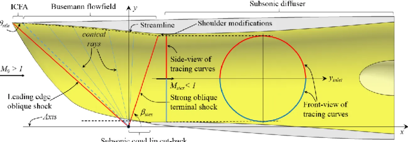
The design of the inlet and the generation of the geometry was performed using the SUPIN (Supersonic Inlet Design and Analysis) tool.[7] The axisymmetric parent flowfield for the STEX inlet was established using the Otto-ICFA-Busemann method.[2] The internal angle of the leading edge was θstle = -5.0 degrees. The parent flowfield
contained a leading, weak oblique shock followed by an isentropic supersonic compression which ended with a strong oblique shock with a shock angle of βstex which decelerated the flow to Mstex = 0.9 and turned the flow into the axial
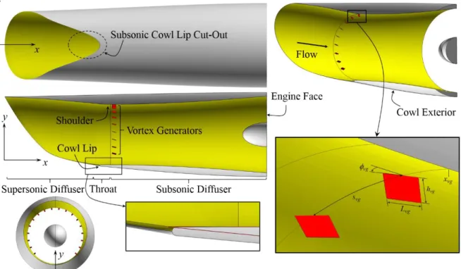
direction. Figure 2 shows a side-view of the inlet along with lines representing the shock and Mach waves of the parent flowfield. The surface of the external supersonic diffuser was created by tracing streamlines in the upstream direction through the parent flowfield starting from circular tracing curves located at the outflow of the parent flowfield, as shown in Fig. 2. The center of the circular tracing curves was offset from the axis-of-symmetry of the parent flowfield, which resulted in a scarfed leading edge for the external supersonic diffuser. The shoulder of the inlet indicated the start of the subsonic diffuser at x = 0.387 ft where the origin of the coordinate x = 0.0 ft was located at the origin of the axisymmetric parent flowfield. The circumferential black curve shown in Fig. 1 indicates the location of the shoulder and start of the subsonic diffuser. The shoulder was rounded slightly to aid the turning of the subsonic flow into the subsonic diffuser. In addition, the cross-sectional area at the shoulder was increased to account for the displacement thickness of the boundary layer. In Fig. 2, this is illustrated by the profile of the inlet being above the dashed curve of the streamline generated by the tracing curve. The throat also featured a “cut-out” at the bottom of the leading edge of the inlet. This cut-out allowed for greater subsonic spillage downstream of the terminal shock, which allowed for the smooth positioning of the terminal shock with change in inlet flow rate.[3] The subsonic diffuser was axisymmetric about the inlet axis and had a length of 2.0 ft. The equivalent conical angle for the subsonic diffuser was 2.94 degrees.
The STEX inlet of Fig. 1 had a blunter cowl lip at the cut-out than the STEX inlets of Refs. [3] and [5]. The cowl lip thickness was increased from 0.001 ft to 0.016 ft to improve the flow as it spilled past the cowl lip.[4] The increased bluntness also improved the structural robustness of the mechanical design of the inlet model for wind-tunnel testing. Figure 1 shows the change in the profiles of the cowl lip with the original cowl lip profile shown in red.
The STEX inlet had a capture area of 0.6006 ft2 and inlet length of 3.353 ft. The reference capture flow rate was
computed as Wcap = 0.9458 slugs/s. The engine flow rate (W2) at the design conditions equaled the reference capture
flow rate. The inlet total pressure recovery computed by SUPIN accounted for losses in the total pressure through the shock waves and subsonic viscous dissipation and had a value of pt2/pt0 = 0.9398.
The STEX inlet is classified as an external-compression inlet because the terminal shock is detached from the cowl lip and subsonic flow downstream of the terminal shock can spill past the cowl lip at all inlet operating conditions.
4
American Institute of Aeronautics and Astronautics
However, it is recognized that the streamline-traced, external supersonic diffuser envelopes much of the exterior supersonic compression, which suggests some internal-compression character for the inlet.
The use of vane-type vortex generators placed just downstream of the shoulder was studied to examine if regions of low-momentum flow in the subsonic diffuser could be reduced. The objectives were to reduce viscous dissipation of the overall flow so as to increase the inlet total pressure recovery and redistribute the flow so as to reduce total pressure distortion at the engine face. The vortex generator geometry was modeled as a rectangular flat plate with a height (hvg) and length (Lvg), which formed an aspect ratio of Lvg/hvg. The vortex generator height was expressed
relative to the local thickness of the boundary layer at the symmetry plane (hvg/). The axial placement of the vortex
generators within the subsonic diffuser was designated xvg with the midpoint of the length of the vortex generators
placed at that axial location. The vortex generators were distributed about a circumferential extent with a spacing of svg. The vortex generators where oriented with an angle-of-incidence vg relative to the inlet axis. Figure 1 shows the
starboard half of the inlet with the geometric factors identified and a vortex generator array in which the vortex generators have a positive angle-of-incidence.
A baseline vortex generator array was established using the results presented in Ref. [5] along with other CFD simulations performed since the presentation of Ref. [5]. The baseline vortex generator array had the properties of hvg/ = 1.0, svg/hvg = 4.0, Lvg/hvg = 2, vg = -16 degrees, and xvg = 0.4327 ft. The boundary layer height used for the
baseline vortex generator array was obtained from CFD simulations of the STEX inlet with no vortex generators and measured at the upper interior symmetry plane to be = 0.026 ft. This resulted in hvg = 0.026 ft and Lvg = 0.520 ft.
The vortex generators were distributed over a circumferential extent of approximately 70% of the upper interior circumference of the inlet at xvg. The circumferential extent was selected to redistribute the low-momentum region,
but limit the vortex generation toward the bottom of the diffuser. The selected circumferential extent resulted in nine vortex generators for each half of the inlet for the baseline vortex generator array. The vortex generators were mirrored about the vertical plane-of-symmetry. Figure 1 shows the vortex generator array.
It was mentioned in the previous section that the boundary layers were thinner along the interior sides and bottom of the throat section due to the scarfing of the leading edge of the inlet. Thus, the bottom-most vortex generators of the baseline array had a height that was about 50% greater than the local boundary layer height. This suggests that a better approach would be to reduce the heights of the vortex generators as they were distributed along the circumference from the top to bottom of the inlet. However, this approach was not explored and remains to be studied in the future.
5
American Institute of Aeronautics and Astronautics III. CFD Simulation Methods
The CFD simulations were performed using the Wind-US CFD flow solver, which is discussed in the next sub-section. Subsequent sub-sections discuss the modeling of the flow domain and boundary conditions for the STEX inlet, generation of the grid, modeling of the vortex generators, refinement of the grids, flowfield initialization, and monitoring of the flow solution for iterative convergence.
A. Wind-US Flow Solver
The Wind-US CFD code [8] was used to solve the steady-state, Reynolds-averaged Navier-Stokes (RANS) equations for the flow properties at the grid points of a multi-block, structured grid defining a flow domain about the STEX inlet. Wind-US used a cell-vertex, finite-volume representation for which the flow solution was located at the grid points and a finite-volume cell was formulated about the grid point. In Wind-US, the RANS equations were solved for the steady-state flow solution using an implicit time-marching algorithm with a first-order, implicit Euler method using local time-stepping from an initial flow solution. All of the simulations were performed assuming calorically-perfect air. The inviscid fluxes of the RANS equations were modeled using a second-order, upwind Roe flux-difference splitting method. The flow simulation can assume inviscid flow, as well as, viscous laminar or turbulent flow. For turbulent flow, the turbulent eddy viscosity was calculated using either the one-equation Spalart-Allmaras (SA) [9] or two-equation Menter Shear-Stress Transport (SST) [10] turbulence models.
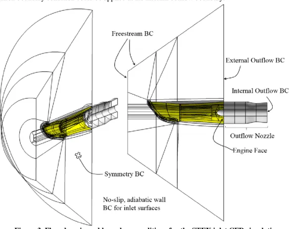
B. Computational Flow Domain and Boundary Conditions
Figure 3 shows the computational flow domain and boundary conditions (BC) used for the CFD simulations of the STEX inlet. The flow domain defined the control volume in which the RANS equations were solved. The flow domain only contained the starboard half of the inlet since the inlet had geometric symmetry about the vertical plane through the center of the inlet and flow symmetry was assumed. Symmetry or reflective boundary conditions were imposed at the symmetry boundary. The internal and external surfaces of the inlet formed a portion of the boundary of the flow domain where non-slip, adiabatic viscous wall boundary conditions were imposed. The inflow and farfield boundaries of the flow domain had freestream boundary conditions imposed in which the Mach number, pressure, temperature, and angle-of-attack were specified. The inflow and farfield boundaries were positioned just upstream of the leading edge oblique shock so that the uniform freestream conditions could be imposed on those boundaries. At the downstream end of the cowl exterior, the domain had an external outflow boundary where an extrapolation boundary condition was applied for supersonic outflow.
Downstream of the engine face, a converging-diverging, outflow nozzle section was added to the flow domain to set the flow rate within the inlet. The nozzle section moved the internal outflow boundary condition downstream of the engine face, which reduced possible interference from the boundary condition on the flow at the engine face. The outflow nozzle is shown in Fig. 3. The converging-diverging portion is preceded by a portion of constant-area. The length of the outflow nozzle section was twice the diameter of the engine face, which was found sufficient for this inlet. A longer length may be required for an inlet in which significant boundary-layer separation extends into the engine face. The cross-sectional area of the throat was set by specifying the ratio of the diameter of the nozzle throat to the diameter of the engine-face (Dnoz/D2) and was set to form choked flow at the throat. Upstream of the nozzle
throat and into the subsonic diffuser, the flow was subsonic and created the necessary back-pressure to support the Figure 2. The features of the axisymmetric, Otto-ICFA-Busemann parent flowfield for the STEX inlet.
6
American Institute of Aeronautics and Astronautics
strong oblique shock at the inlet throat section. Reducing the outflow nozzle throat area increased the back-pressure, and so, reduced the inlet flow rate. Downstream of the outflow nozzle throat, the flow was supersonic, and so, an extrapolation boundary condition could be applied at the internal outflow boundary.
Figure 3. Flow domain and boundary conditions for the STEX inlet CFD simulations. C. Computational Grid
The computational grid for the flow domain was generated by dividing the flow domain into multiple blocks and generating structured grids for each block. The SUPIN tool was used to generate the blocks and grid points using a fairly automated process. SUPIN also created the boundary condition file for the Wind-US CFD flow solver. The inputs to the process include some factors to determine the extents of the flow domain and spaces between grid points. The grid spacing factors include the grid spacing of the first grid point away from the wall (swall), grid spacing within
the throat section in the streamwise direction (sx), and grid spacing in the circumferential direction (sc). SUPIN
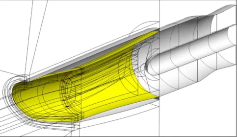
then imposed these grid spacing values along the edges of the inlet geometry and flow domain to compute the required number of grid points along those edges. A grid block topology was assumed for the STEX inlet to form the edges into faces and those faces into blocks. SUPIN generated grids along the edges, on the surfaces, and within the interior volume of each block. The interior block boundaries abutted with other block boundaries. For most blocks, the grid lines were contiguous across block boundaries, but some non-contiguous boundaries were used to facilitate the structured topology. Figures 3 and 4 shows an example of the flow domain with the multi-block topology. Figure 5 shows an example of the grid lines for the block faces on the symmetry boundary. The red and blue colors indicate individual faces of blocks.
7
American Institute of Aeronautics and Astronautics D. Vortex Generator Modeling
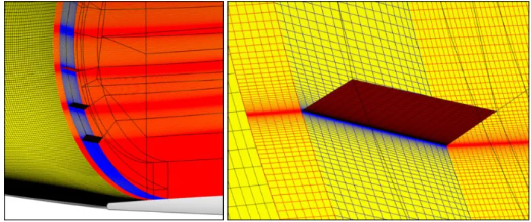
The vortex generators were modeled using either the Bender-Anderson-Yagle (BAY) vortex generator model [11,12] within the Wind-US flow solver or using multi-block grids directly generated about the vortex generators. The BAY vortex generator model approximated the lift force generated by each vortex generator and used the lift force in the momentum and energy equations for the grid points about the vortex generator. The local flow velocity was also aligned with the vortex generator angle-of-incidence. The specification of a vortex generator with the BAY model required indicating the three-dimensional region of grid points which contained the vortex generator. Figure 6 shows an example of one vane-type vortex generator near the bottom of the inlet along with the region of grid points that enclosed the vortex generator. Additional input specifications include the planform area and angle-of-incidence of the vortex generator.
Figure 4. Structured, multi-block grid topology about the STEX inlet and the vane-type vortex generators.
Figure 5. Structured, multi-block, computational grids on the symmetry plane for the STEX inlet with computational grids about the vortex generators.
8
American Institute of Aeronautics and Astronautics
An alternative to the use of the BAY vortex generator model was to directly generate multi-block grids about the vortex generators. This approach was used and demonstrated in Ref. [13] for ramp and vane-type vortex generators within a two-dimensional inlet. The grid generation was performed using SUPIN in much the same manner as the generation of the grids described above. Additional factors were specified for the streamwise and spanwise grid spacing along the vortex generator. Figures 4 and 5 showed the blocks about a vortex generator array within the flow domain. Figure 7 shows more of the details of the blocks and surface grid generation about the vortex generators. The vortex generators were modeled as flat plates of zero thickness and each vortex generator formed a face between two blocks so that non-slip (viscous), adiabatic wall boundary conditions could be applied. With the vortex generator at an angle-of-incidence to the local flow, a pressure differential was created, which created the vortex.
E. Refined Grids
The automated grid generation process within SUPIN simplified the generation of a series of computational grids used for the grid refinement study to be discussed in Section IV. Eight grids were generated with various lengths for the grid spacing factors discussed above. Table 1 lists the input factors and properties of the grids. The two key factors were the axial and circumferential grid spacing values that are normalized by the engine-face diameter, sx/D2
and sc/D2, respectively. For all of the grids, the spacing for the first grid point off the wall was kept the same at swall
= 8.0E-06 ft so that the non-dimensional boundary-layer coordinate of the first grid point was y+ 1 so as to properly
resolve the boundary layer. Table 1 lists the resulting number of grid points within the internal duct of the inlet in the axial (Nx), radial (Nr), and circumferential (Nc) directions for each grid. The number of axial grid points (Nx) is the
number of grid points from the start of the inlet to the engine face. The number of radial grid points (Nr) is the number
of grid points from the bottom to the top of the inlet duct. The number of circumferential grid points (Nc) is the number
of grid points about the circumference of the internal duct for the starboard half of the inlet included in the computational flow domain. The Ngint is the total number of grid points within the interior duct of the inlet, which is
considered the region from the leading edge of the inlet to the engine face. The value listed in the column labeled Ngint of Table 1 is in millions of grid points. The BAY model was the only vortex generator model used with grids
Figure 6. The STEX inlet with a grid region enclosing a vortex generator used for specifying the region for application of the BAY vortex generator model.
Figure 7. Structured, multi-block, surface grid about the vane-type vortex generators within the STEX inlet.
9
American Institute of Aeronautics and Astronautics
A, B, C, D, and E. Grids F and G included multi-block grids generated about the baseline vortex generator array. Grid H had multi-block grids generated about an alternative vortex generator array with smaller vortex generators.
The grid convergence study will use an equivalent grid spacing (sEQ/D2) that was computed as the
root-mean-square of the normalized axial, radial, and circumferential grid spacings and is listed in Table 1. Also listed in Table 1 is the normalized equivalent grid spacing (hn), which is the equivalent grid spacing for the respective grid divided
by the equivalent grid spacing for grid G, which was the minimum value of the all eight grids.
Grid sx/D2 sc/D2 Nx Nr Nc Ngint (x106) sEQ/D2 hn A 0.020 0.030 272 184 85 2.02 0.028 5.40 B 0.015 0.024 328 194 103 2.99 0.022 4.25 C 0.010 0.017 431 217 147 5.76 0.015 2.95 D 0.005 0.010 744 278 247 18.1 0.008 1.63 E 0.005 0.005 582 384 497 34.3 0.007 1.45 F 0.005 0.010 422 334 724 21.8 0.008 1.47 G 0.003 0.005 733 395 1080 68.9 0.005 1.00 H 0.005 0.009 465 346 948 31.3 0.007 1.45
F. Initial Flow Solution and Solution Monitoring
The CFD simulations were initialized with a flowfield set to the freestream conditions. The simulation started with the first-order form of the Roe flux-splitting method so as to damp out large initial gradients. Eventually, the second-order flux method was applied as the residuals over the iterations decreased and the boundary layers, shock waves, and subsonic inlet flow took form. At the start of the simulations, the Courant-Friedrichs-Lewy (CFL) number had a value of 0.5, but increased incrementally to a value of 2.5 as the flow solution developed. Local time stepping was used in which the local time step used was computed based on the CFL number and the local grid cell size. The iterative convergence was indicated in part by the reduction of the root-mean-square of the residuals of the conservative variables for each block. Iterative convergence was also evaluated through the monitoring of the convergence of the inlet flow rate, total pressure recovery, and total pressure distortion. The steady-state solution was considered converged when these values varied less than 0.1% of their values over 1000-2000 iterations.
G. Inlet Performance Metrics
The flow solutions from the CFD simulations were used to obtain the aerodynamic performance metrics of the STEX inlet. The four inlet performance metrics used to characterize the inlet included the 1) inlet flow ratio (W2/Wcap),
2) inlet total pressure recovery (pt2/pt0), 3) General Electric (GE) inlet circumferential distortion index (IDC), and 4)
GE inlet radial distortion index (IDR). The inlet flow ratio was defined as the inlet flow rate (W2) divided by the
reference capture flow rate (Wcap). The inlet flow rate (W2) was obtained from a CFD simulation by integrating the
rate of flow passing through the cross-stream grid planes of the outflow nozzle. The total pressure at the engine face (pt2) was computed as the mass-average of the total pressures at the grid plane at the engine face.
The third and fourth metrics of inlet performance were indices of the inlet circumferential (IDC) and radial (IDR) total pressure distortion at the engine face as defined by General Electric.[14] The distortion indices were defined on a standard 40-probe rake array of the Society of Automotive Engineers (SAE) Aerospace Recommended Practices (ARP) 1420 document.[15] The rake array consisted of eight radial rakes each containing five total pressure probes. In the circumferential direction the eight probes were located at a constant radius and formed a ring about the circumference of the engine face. Each ring was placed radially at the centroid of equal-area sectors. The middle-right image of Fig. 8 shows the total pressure recovery contours for a CFD simulation along with the probe locations indicated by white circles. Only 25 probes of the 40-probe rake are shown for the half of the engine face included in the computational flow domain. The flowfield from the CFD simulation was interpolated onto the locations of the probes to obtain the total pressure at the probe location. The IDR index is identical to the radial distortion index defined in the SAE ARP 1420, Ref. [15]. The method for computation of the IDC index for each ring can be found in Ref. [14]. The IDC indices reported in this paper were computed as the average of the IDC indices computed on the two outer rings because for the STEX inlet, the total pressure distortion was predominately a tip distortion.
10
American Institute of Aeronautics and Astronautics
IV.
Results
This section presents results from CFD simulations of the STEX inlet without and with vortex generators. The results examine the grid convergence of the CFD simulations and the influence of turbulence modeling, vortex generator modeling, and vortex generator size on the inlet performance.
A. Clean STEX Inlet
CFD simulations were performed to characterize the inherent flow and performance of the “clean” STEX inlet with no vortex generators. Simulations were performed using both the Menter SST and Spalart-Allmaras turbulence models. Table 2 lists the grids that were used for the simulations for each outflow nozzle setting. The “N” is the number of simulations for each outflow nozzle setting. The “t” is the t-statistic, which will be discussed later.
Nozzle Setting Menter SST Spalart-Allmaras
Dnoz / D2 N Grids t (95%,N-1) N Grids t (95%,N-1)
0.858 4 A,B,C,D 3.182 4 A,B,C,D 3.182 0.856 8 A,B,C,D,E,F,G,H 2.365 4 A,B,C,D 3.182 0.854 8 A,B,C,D,E,F,G,H 2.365 4 A,B,C,D 3.182 0.853 7 A,B,C,D,E,F,G 2.447 4 A,B,C,D 3.182 0.852 6 A,B,C,D,E,G 2.571 4 A,B,C,D 3.182 0.851 4 A,B,C,D 3.182 4 A,B,C,D 3.182 0.850 4 A,B,C,D 3.182 4 A,B,C,D 3.182
Figure 8 shows Mach number and total pressure contours from the CFD simulation on grid D at three levels of inlet flow ratio. The images illustrate the key features of the STEX inlet flowfield. The middle row of images show the inlet flowfield for an outflow nozzle setting of Dnoz/D2 = 0.854, which was near the critical operating condition for
which the inlet is operating at its design condition and near its maximum inlet flow ratio and total pressure recovery. The left column of images of Fig. 8 show the Mach number contours on the symmetry plane. The leading edge oblique shock descends from left to right at a shock angle of approximate -45 degrees and passes ahead of the cowl lip. The Mach numbers decrease along the external supersonic diffuser in the streamwise direction as part of the supersonic isentropic compression. The terminal shock wraps around the cowl lip and intersects the external supersonic diffuser just upstream of the shoulder. The offset of the terminal shock forward of the cowl lip indicates subsonic spillage. Downstream of the terminal shock, the internal flow becomes subsonic and the Mach number decreases as the flow is diffused approaching the engine face. The interaction of the terminal shock with the shoulder creates a region of low-momentum flow that extends into the top of the subsonic diffuser and to the engine face. The second column of images shows the Mach number contours at four axial stations within the subsonic diffuser. The growth of the low-momentum region can be seen as the increase in the darker blue regions. The third and fourth columns of Fig. 8 show the Mach number and total pressure recovery contours, respectively, at the engine face. At the right of Fig. 8 is listed the mass-averaged Mach number at the engine face, which corresponds to the corrected flow rate of the engine face, and the inlet performance metrics for each flowfield.
The top row of images show the inlet flowfield for an outflow nozzle setting of Dnoz/D2 = 0.852, which resulted in
a subcritical operating condition in which the inlet flow ratio was below the critical operating inlet flow ratio. As can be seen, the terminal shock was pushed forward to allow a greater amount of subsonic spillage past the cowl lip. The bottom row of images show the inlet flowfield for an outflow nozzle setting of Dnoz/D2 = 0.858, which resulted in a
supercritical operating condition in which the terminal shock was drawn slightly into the throat section of the inlet as the internal ducting of the inlet approaches a choked condition of maximum flow. The inlet total pressure recovery was reduced as the extent of the momentum region increased for supercritical operation. The larger low-momentum region at the top of the engine face resulted in greater radial distortion.
The characteristic curves obtained from the CFD simulations of the clean inlet with the Menter SST turbulence model are shown on the left-side of Fig. 9. The top-left image shows the curves of the total pressure recovery with respect to the inlet flow ratio. The critical operating condition is the point on the curve for which the inlet flow ratio has reached its maximum value while still achieving near its maximum total pressure recovery. The supercritical region is characterized by near constant inlet flow ratio with a decrease in the total pressure recovery as the inlet corrected flow rate increases. The subcritical region is characterized by a gradual decrease in the total pressure recovery as the inlet flow ratio decreases. The middle-left image shows the curves of the circumferential distortion with respect to the inlet flow ratio. Within the subcritical region, the circumferential distortion increases slightly with
Table 2. Listing of the outflow nozzle settings and grids for CFD simulations of the clean STEX inlet.
11
American Institute of Aeronautics and Astronautics
increase in the inlet flow rate; however, within the supercritical region, the circumferential distortion sharply increases. The bottom-left image shows the curves for the radial distortion and shows a rather flat variation with respect to the inlet flow ratio. As an indication of acceptable values of the circumferential and radial distortion, Ref. [16] indicates stability limits for the General Electric F404-GE-400 turbofan engine as IDC < 0.2 and IDR < 0.1. Thus, decreasing the values of the radial distortion seem to be the higher priority for the STEX inlet.
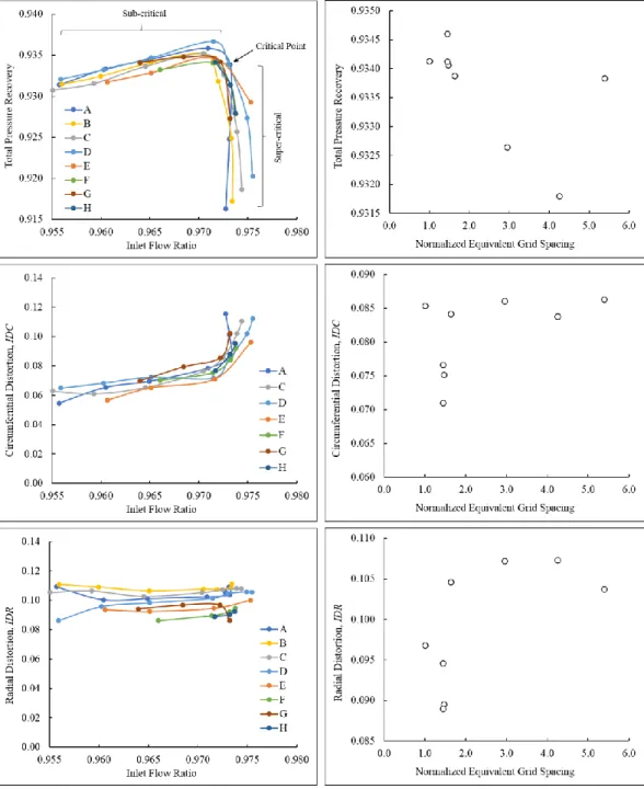
The characteristic curves shown on the left-side of Fig. 9 show similar behavior for all of the grids and fall within a coherent band. The expected behavior of the performance metrics with respect to grid refinement is that the inlet performance metrics for each outflow nozzle setting would approach an asymptotic value in a smooth and monotonic manner as the grid is refined. To examine this, the plots on the right-hand-side of Fig. 9 show the variation of the performance metrics from the CFD simulations with the Menter SST turbulence model for the outflow nozzle setting Dnoz/D2 = 0.854 with respect to the normalized equivalent grid spacing (hn) listed in Table 1 for each grid. The
upper-right plot does seem to suggest that the total pressure recovery approaches a value of about pt2/pt0 = 0.9340; however,
the convergence is not smooth. The change in value between the maximum and minimum values of total pressure recovery are pt2/pt0 0.0028. The plots for the circumferential and radial distortion on the right-hand-side of Fig. 9
show most of the variation with the smallest levels of grid refinement. In addition, these changes in value reach levels of IDC 0.015 and IDR 0.018, which approach approximately 20% of the average values of these quantities.
The grid convergence behavior for the other outflow nozzle settings likewise do not provide a smooth and monotonic grid convergence. This can be seen by how the characteristic curves on the left-hand-side of Fig. 9 weave among the other curves and defy a sensible description of the behavior of the inlet performance metrics with grid refinement. This behavior seems to suggest that there is some source of noise in the CFD simulations.
One possible source is the level of iterative convergence. The iterative convergence was indicated in Section II to be less than 0.1% for the performance metrics. For the total pressure recovery, this amounts to pt2/pt0 = 0.0010,
which is on the same order as the change described above. Thus, iterative convergence to a level of 0.01% may be more appropriate if one wishes to observe grid convergence with changes of pt2/pt0 0.0001. This was achieved for
some CFD simulations, but care is needed to ensure all CFD simulations reach this level.
Another source of noise may be the behavior of the inlet flow ratio with grid refinement. For the CFD simulations of Fig. 9 at Dnoz/D2 = 0.854, the changes in the inlet flow ratio reached levels of W2/Wcap 0.0018. As the inlet flow
ratio varies, the solution point moves along the characteristic curves. Thus a change in the inlet flow ratio also results in a change in the inlet performance metrics.
For the distortion metrics, a source of noise may be the interpolation onto the probes of the rakes. The values of the total pressure at the probes are interpolated from the CFD solution. If the distortion is very localized and prone to movement depending on the level of grid refinement, then relatively large changes at a probe location may be possible. A better approach would be to perform a mass-averaging of the grid points falling within the equal-area segment associated with the probe. This would reduce variations due to point interpolation of a localized distortion.
Figure 8. Mach number and total pressure contours from CFD simulations on grid D for three levels of inlet flow ratio.
12
American Institute of Aeronautics and Astronautics
The comparison of the characteristic curves generated using the Menter SST and Spalart-Allmaras turbulence models are presented in the left-hand-side of Fig. 10 for CFD simulations using grids B, C, and D. Grids B, C, and D were generated in the same manner with the only inputs being changed were grid spacing within the throat section in the streamwise direction (sx) and the grid spacing in the circumferential direction (sc). Grid A was similarly
generated; but are not shown in Fig. 10. The characteristic curves for the Menter SST model are the same as those presented in Fig. 9.
One observation from the supercritical region of the characteristic curves for the total pressure is that as the grid is refined, the tendency is for the inlet flow ratio and the total pressure recovery to increase. This behavior may temper over-optimistic estimates of these values for lower levels of grid refinement. The circumferential distortion seems to increase with grid refinement while the radial distortion decreases with grid refinement.
Figure 9. Characteristic curves for the clean inlet with the SST turbulence model (left) and the variations of the performance metrics with respect to the normalized equivalent grid spacing for nozzle setting Dnoz/D2 = 0.854 (right).
13
American Institute of Aeronautics and Astronautics
The characteristic curves for the total pressure recovery from the CFD simulations using the Spalart-Allmaras turbulence model show higher values for the total pressure than those from CFD simulations using the Menter SST turbulence model. The Menter SST turbulence model seems to be indicating higher values of viscous dissipation leading to greater total pressure losses within the inlet, especially within the subcritical region. The inlet flow does not have regions of boundary-layer separation, so the expectation is that both turbulence models should calculate similar levels of turbulent viscosity.
The first approach for quantifying the uncertainty uses the standard statistical methods for calculating a confidence interval. Such methods were demonstrated in Ref. [17]. The confidence interval for a performance metric Y is computed as
𝑌 = 𝑌̅ ±𝑡(95%, 𝑁 − 1) 𝑆
√𝑁 = 𝑌̅ ± ∆𝑌 (1)
The t is the critical value from the t-distribution for a 95% confidence level with N-1 degrees-of-freedom. Table 2 listed the respective t-statistic for each nozzle setting and turbulence model. The S is the standard deviation calculated as the square-root of the variance calculated as
𝑆2=∑𝑁𝑖=1(𝑌𝑖− 𝑌̅)2
𝑁 − 1 (2)
The S2 is the variance of the sample of N performance metrics denoted as Y i.
The 𝑌̅ is an average of the inlet performance metric. The approach taken here is to accept that there does not seem to be a smooth and asymptotic value for the inlet performance metric at each outflow nozzle setting, as discussed above and shown in Figs. 9 and 10. Thus, the approach is to simply take an average of all values of the respective performance metric for an outflow nozzle setting. Thus, for the outflow nozzle setting of Dnoz/D2 = 0.854, an average
is calculated for all N = 8 values of the respective inlet performance metric obtained from the CFD simulations using the Menter SST turbulence model. The variance is then calculated using Eq. 2 and the confidence interval is then calculated using Eq. 1. This is repeated for the performance metrics from the CFD simulations for all of the outflow nozzle settings and for both turbulence models.
The averaging creates a set of averaged characteristic curves and their respective curves for the confidence intervals, as shown in the plots on the right-hand-side of Fig. 10. The process implies that there is a 95% confidence in the grid refinement that the value of the inlet performance metric lies within the bounds of the confidence interval curves. Table 3 lists the confidence intervals computed for each performance metric for each outflow nozzle setting and both turbulence models.
The differences in the performance metrics with respect to the turbulence models adds uncertainty to the values of the performance metrics. In general, the Menter SST turbulence model indicates lower values of the total pressure recovery and higher values of the distortion than those from the use of the Spalart-Allmaras turbulence model. The differences in the inlet performance metrics are as great as pt2/pt0 0.006, IDC 0.007, and IDR 0.007 over
portions of the average characteristic curves. The difference for the total pressure recovery is of concern, and require further study. The differences for the distortion metrics seem to be within the uncertainties of the grid refinement.
Nozzle Setting ∆𝒀/𝒀̅ (Menter SST) ∆𝒀/𝒀̅ (Spalart-Allmaras)
Dnoz / D2 pt2/pt0 IDC IDR pt2/pt0 IDC IDR 0.858 0.30% 6.00% 3.98% 0.24% 6.09% 3.34% 0.856 0.14% 3.24% 7.18% 0.26% 3.13% 5.23% 0.854 0.08% 6.10% 6.41% 0.23% 3.98% 2.13% 0.853 0.13% 6.42% 7.04% 0.16% 2.23% 2.27% 0.852 0.12% 9.01% 5.24% 0.12% 8.51% 3.35% 0.851 0.14% 12.85% 9.17% 0.14% 11.42% 7.77% 0.850 0.09% 16.04% 17.57% 0.10% 27.68% 8.41% Table 3. Normalized confidence intervals for the inlet performance metrics for CFD simulations of the clean STEX inlet.
14
American Institute of Aeronautics and Astronautics
Another approach for examining and reporting the results of a grid refinement study is the use of the grid convergence index (GCI).[18,19] The GCI is based on a general Richardson extrapolation with the objective of providing a measure of the uncertainty of the grid convergence. The Richardson extrapolation attempts to obtain the asymptotic value of a quantity as the grid spacing approaches zero. The GCI is a measure of the percentage that the computed value differs from the asymptotic value and how much the value would change with further grid refinement. As it was shown in Fig. 9, the performance metrics did not show a smooth and monotonic behavior, and so, the calculation of the grid convergence indices requires some approximations. Here we use grid D as the fine grid and grid C for the course grid. The GCI is then calculated as
𝐺𝐶𝐼𝐶𝐷=
𝐹𝑆 |(𝑌𝐷− 𝑌𝐶) 𝑌⁄ |𝐷
𝑟𝐶𝐷𝑝 − 1 (3)
Figure 10. Characteristic curves for the clean STEX inlet for grids B, C, and D (left) and the averaged characteristic curves with their confidence intervals (right).
15
American Institute of Aeronautics and Astronautics
The FS is the factor of safety for the calculation, and a value of FS = 3.0 is used here to be conservative. The YC and
YD are the values of the inlet performance metric for grids C and D, respectively. The rCD is the grid refinement ratios
calculated using the values of hn from Table 1 to be rCD = 2.95 / 1.63 = 1.81. The p is the order of convergence and a
value of p = 2.0 is assumed, which implies second-order numerical methods.
Table 4 lists the grid convergence indices computed for grid D for the inlet performance metrics from the CFD simulations using the Menter SST and the Spalart-Allmaras turbulence models. It seems reasonable to state that most of the GCI values for the total pressure recovery are well below 1% and indicate grid convergence with respect to that metric, at least for engineering design. For the IDC and IDR distortion indices, most of the GCI values are less than 2% to 8%.
Nozzle Setting GCICD (Menter SST) GCICD (Spalart-Allmaras)
Dnoz / D2 pt2/pt0 IDC IDR pt2/pt0 IDC IDR 0.858 0.23% 2.01% 2.88% 0.18% 1.65% 1.35% 0.856 0.24% 0.06% 2.63% 0.11% 3.84% 8.81% 0.854 0.18% 2.99% 3.29% 0.20% 1.42% 3.49% 0.853 0.21% 8.40% 5.09% 0.16% 0.16% 3.24% 0.852 0.14% 12.82% 5.79% 0.17% 8.57% 4.72% 0.851 0.24% 14.25% 14.65% 0.25% 14.88% 8.62% 0.850 0.19% 4.28% 29.49% 0.17% 27.63% 7.68% B. Baseline Vortex Generator Array with the BAY Model
CFD simulations were performed for the STEX inlet with the baseline vortex generator array modeled using the BAY vortex generator model. As with the clean STEX inlet simulations, the results obtained using grids B, C, and D and the Menter SST and Spalart-Allmaras turbulence models are presented here to provide a consistent comparison to the results of the previous section. In addition, results using grid E are also plotted.
Figure 11 shows the Mach number and total pressure recovery contours from a simulation performed with grid D and the Menter SST turbulence model. The images are for a nozzle setting of Dnoz/D2 = 0.854. The bottom-left image
shows the Mach number contours at five axial stations. The effects of the vortex generators are seen with the formation and diffusion of vortices about each vortex generator. In comparison to the images of Fig. 8 for the clean STEX inlet, the images of Fig. 11 indicate that the low-momentum flow at the top of the subsonic diffuser in Fig. 8 has been distributed downward along the sides of the subsonic diffuser. However, a rather sizable vortex formed near the bottom of the subsonic diffuser as a result of the accumulation of the co-rotating vortices. This represents a localized swirl in the flow, which could be of concern to a turbo-fan engine.
Table 4. Grid convergence indices for the CFD simulations of the clean STEX inlet.
Figure 11. Mach number and total pressure contours for the baseline vortex-generator array modeled using the BAY vortex generator model with grid D.
16
American Institute of Aeronautics and Astronautics
The characteristic curves for the inlet performance for each grid and turbulence models are plotted on the left-hand-side of Fig. 12. An observation is that curves for the inlet total pressure and the circumferential distortion from the simulations with grid B are different than those with grids C and D. The characteristic curves for the radial distortion do not show much difference. It was concluded that grid B was too coarse to adequately capture the formation and propagation of the vortices of the vortex generators. Another observation was that there did not seem to be a sizable difference between the use of the Menter SST and the Spalart-Allmaras turbulence models. As with the results of the previous section, an overall characteristic curve was obtained by averaging the values of the inlet performance metrics for each nozzle setting. Here, the averages included the values of both turbulence models. The plots on the right-hand-side of Fig. 12 show the resulting characteristic curve for each inlet performance metric with the label “Baseline VGs. BAY”. Also included on the right-hand-side plots are the characteristic curves for the clean STEX inlet. The plots of the characteristic curves on the right-hand-side of Fig. 12 suggest that the baseline vortex generator array increased the total pressure recovery and inlet flow ratio near the critical operating condition. Further, the plots indicate that the vortex generator array reduced both circumferential and radial distortion.
The uncertainties with respect to the grid refinement were computed using both approaches as discussed in the previous section. Table 5 lists the normalized confidence intervals and the grid convergence indices for the CFD simulations on grids C and D of the STEX inlet with the baseline vortex generators modeled using the BAY model and the Menter SST turbulence model. As with the GCI values with the clean inlet simulations, the values of the inlet total pressure recovery show low GCI values with the values for the distortion indices indicating higher values and more variation.
Nozzle Setting ∆𝒀/𝒀̅ GCICD
Dnoz / D2 pt2/pt0 IDC IDR pt2/pt0 IDC IDR 0.858 0.17% 25.45% 7.91% 0.28% 55.57% 7.37% 0.856 0.19% 43.28% 7.53% 0.29% 100.83% 8.24% 0.854 0.27% 40.97% 6.06% 0.41% 69.58% 3.13% 0.853 0.42% 52.59% 7.25% 0.00% 89.41% 5.27% 0.852 0.40% 17.64% 3.85% 0.31% 4.26% 1.31% 0.851 0.43% 36.16% 6.23% 0.39% 7.43% 4.30% 0.850 0.46% 37.11% 7.45% 1.00% 30.96% 27.96% Table 5. Normalized confidence intervals and grid convergence indices for the CFD simulations of the STEX inlet with the baseline vortex generators modeled using the BAY model.
17
American Institute of Aeronautics and Astronautics
C. Baseline Vortex Generator Array with Grids Generated about the Vortex Generators
CFD simulations were performed for the STEX inlet with the baseline vortex generator array in which multi-block grids were generated about each vortex generator. The simulations involved grids F and G of Table 1. The Menter SST turbulence model was used for all of these CFD simulations. Figure 13 shows Mach number and total pressure recovery contours from a CFD simulation using grid G for a flowfield that with the outflow nozzle setting of Dnoz/D2
= 0.855. The images can be compared to those of Fig. 11 that used the BAY vortex generator model. The grid about the vortex generator provided greater resolution of the formation and initial propagation of the vortex compared to the use of the BAY model. As with the previous section, the vortex generator array redistributed the low-momentum flow about the circumference of the subsonic diffuser and formed a vortex near the bottom of the subsonic diffuser. The solution with the grids about the vortex generators is more subcritical than that with use of the BAY model.
Figure 12. Characteristic curves for the STEX inlet with the baseline vortex generators modeled using the BAY vortex generator model.
18
American Institute of Aeronautics and Astronautics
Figure 14 shows the inlet characteristic curves for these simulations. The simulation from which the images of Fig. 13 were obtained is indicated by the note and label. Also plotted in Fig. 14 are the curves from Fig. 10 for the clean inlet for both the Menter SST and the Spalart-Allmaras turbulence models and the curve from Fig. 12 for the inlet with the vortex generators modeled with the BAY model. All of these curves use the same outflow nozzle settings. An observation is that with the use of the grid blocks about the vortex generators, the total pressure recoveries are much less than those obtained with the use of the BAY model. The total pressure recoveries are even less than those of the clean inlet with the SST turbulence model. The circumferential distortion indices calculated with the grid about the vortex generators likewise are higher than those of the BAY model. Near the critical inlet operation, the gridded vortex generators come close to the performance as calculated by the BAY model. The gridded vortex generators do seem to reduce radial distortion to levels similar to those of the BAY model, but the radial distortion increases at the higher inlet flow ratios.
The BAY model imposes a lifting force on the momentum and energy equations that then results in a vortex, but the model does not account for viscosity. The differences in the total pressure recovery between the use of the BAY model and the use of multi-block grids about the vortex generators were explored with additional CFD simulations. First, simulations were performed with slip-wall or inviscid boundary conditions specified for the surfaces of the vortex generators. While not physically correct, it allowed an examination of the viscous effects of the vortex generators on the flowfield. Figure 14 shows the resulting characteristic curves. While some differences exist, it seems apparent that viscosity on the vortex generator surfaces does not have a large effect.
With 18 vortex generators in the baseline vortex generator array for the entire inlet, the array presented about 1.4% blockage for the internal flow at the start of the subsonic diffuser. This blockage is calculated as the ratio of the combined area of the forward projection of the vortex generators at vg = -16 degrees angle-of-incidence and the
cross-sectional area at the start of the subsonic diffuser. This blockage may be enough to reduce the inlet flow ratio when multi-block grids are generated about the vortex generators compared to the use of the BAY model. The BAY model may not fully model the effect of having a solid wall within the flowfield causing blockage.
To explore the issue of blockage, a vortex generator array was established in which the vortex generators had heights of about 75% of the local boundary layer height. The spacing and angle-of-incidence of the vortex generators remained the same as the baseline vortex generator array at svg/hvg = 4.0 and vg = -16 degrees, respectively. The
resulting blockage was about 1.0%. Grid H was generated for this vortex generator array and CFD simulations were performed using the same outflow nozzle settings as for grid G. Figure 15 shows the Mach number and total pressure recovery contours for a flow solution for the outflow nozzle setting of Dnoz/D2 = 0.855. The characteristic curves are
included in Fig. 14. The inlet flow ratios of the simulations of grid H were greater and showed less spillage than those of the simulations of grid G. This seems to support the idea that with smaller vortex generators the blockage, and so, the spillage, is less. The total pressure recoveries are slightly higher for the subcritical region. The smaller vortex generators still seem effective in reducing the radial distortion.
Figure 13. Mach number and total pressure contours of the STEX inlet with the baseline vortex generators modeled with grids about the vortex generators (grid G).
19
American Institute of Aeronautics and Astronautics
Figure 14. Characteristic curves for the STEX inlet with the vortex generators modeled with grids about the vortex generators (left) and comparison of the characteristic curves with the vortex generators with viscous and inviscid boundary conditions (right).
20
American Institute of Aeronautics and Astronautics
D. Use of Design-of-Experiments and Response Surface Methods for Vortex Generator Array Design The design of a vortex generator array for the STEX inlet involved a number of geometric factors (e.g., ,xvg, hvg,
Lvg, svg, and vg) that were described in Section II. Reference [5] presented some earlier studies of such factors in the
context of several design-of-experiments (DOE) and statistical response surface methods (RSM) studies. The objective was to establish which factors were the most influential in affecting the desired outcome of increased inlet total pressure recovery and reduced circumferential and radial total pressure distortion. The CFD simulations of Ref. [5] used the Wind-US solver and the BAY vortex generator model in a similar manner as described above. The results of those studies were summarized in Section I. The difficulty encountered in the studies of Ref. [5] was that statistically significant response surface models for the performance metrics could not be constructed. The cause seemed to be that the change in the total pressure recoveries and distortion indices were too small with respect to the level of the noise.
This section discusses an additional DOE and RSM study that was performed to explore if the noise could be reduced such that statistically-significant models could be constructed. The Wind-US solver with the Menter SST turbulence model and the BAY vortex generator model was used for the CFD simulations. With use of the BAY model, a single grid could be used for all of the CFD simulations with each vortex generator array requiring only changes to the Wind-US input data file. The CFD simulations used grid E, which used a refined grid in the circumferential direction for the blocks encompassing the vortex generators.
For the DOE study, the axial position of all of the vortex generator arrays was specified to be just downstream of the shoulder at xvg = 0.4327 ft, which was also the position for the baseline vortex generator array as described in
Section II. Also, as with the baseline vortex generator array, the aspect ratio of the vortex generators was fixed at Lvg/hvg = 2.0. The DOE study involved three factors with three levels for each factor: hvg/ = 0.50, 0.75, and 1.0; vg
= -12, -16, and -20 degrees; and svg/hvg = 3, 4, and 5. The DOE study used a central-composite face-centered design
[20] which resulted in 15 separate vortex generator arrays, which are listed in Table 6 along with the values of the factors for each vortex generator array. The number of vortex generators for each array was determined from the vortex generator height and its relative spacing over the circumference of the inlet. Each array was assumed to span approximately 70% of the circumferential distance of the inlet with the array centered about the top-symmetry boundary of the inlet. Table 6 lists the number of vortex generators (Nvg) for the starboard half of the inlet as modeled
in the CFD flow domain.
It was assumed that the performance metrics from the CFD simulations of each vortex generator array could be compared if the engine-face corrected flow rate was fixed at the design flow rate corresponding to the critical operation of the clean STEX inlet. This would only require 15 CFD simulations corresponding to each of the 15 vortex generator arrays of Table 6. The CFD simulations of Ref. [5] hoped to achieve this condition by using a fixed outflow nozzle throat setting (Dnoz/D2). However, it was found that the corrected flow rate varied up to 5%. This likely was a source
Figure 15. Mach number and total pressure contours for CFD simulations with the smaller vortex generators of grid H.
21
American Institute of Aeronautics and Astronautics
of the noise. For the current DOE study, it was decided to use a subsonic Mach number boundary condition since the corrected flow rate can be expressed equivalently as an average Mach number for the specified engine face. The internal outflow boundary was placed at the start of the converging section of the outflow nozzle. Thus, the outflow was at the end of a straight, constant-area duct downstream of the engine face. The specified Mach number for the boundary condition was MBC = 0.4327, which corresponded to the design condition and the design inlet corrected flow
rate (WC2*). The boundary condition adjusted the local static pressure values at the outflow boundary to match the
mass-averaged Mach number with the specified Mach number (MBC). In this process, the local Mach number was
allowed to vary at the outflow boundary.
The 15 CFD simulations were performed and Table 6 lists the corresponding inlet performance metrics. Also listed in Table 6 is the observed average Mach number at the engine face (M2) and the ratio of the observed and design
corrected flow rates (WC2/WC2*). Most of the CFD simulations were able to maintain the corrected flow rate within
1% of the design corrected flow rate. The simulation for array 4 was the worst case with being about 1.5% different than the design corrected flow rate. Array 4 had the most blockage with the maximum height and angle-of-incidence while having the minimum spacing between the vortex generators.
The variations of the total pressure recoveries listed in Table 6 were small. The difference between the maximum and minimum total pressure recoveries was only 0.87% of the average value, which was of the same scale as the variation of the corrected flow rate. A statistical analysis was performed using Design Expert® [21]; however, the analysis-of-variance methods were not able to form a statistically-significant response surface model for the inlet total pressure recovery. This meant that the DOE study was unable to state within a 95% certainty that the variation in the total pressure recovery was due to any of the vortex generator factors. Thus, the best representation of the total pressure recovery was an average of all 15 values of Table 6, which would result in pt2/pt0 = 0.9387. The response of
the total pressure recovery was overshadowed by the noise of the variations, of which, the variation in the corrected flow rate was a source of the noise. In the previous section, it was shown that the BAY vortex generator model seemed to indicate higher total pressure recoveries than those from CFD simulations with grid blocks about the vortex generators. Thus, it may be reasonable to not expect the vortex generators to increase the total pressure recovery, but rather just hope that the vortex generator array does not adversely reduce the total pressure recovery.
The variations of the circumferential distortion indices varied from a low of IDC = 0.0280 to high of IDC = 0.0592. These values are considered low, as far as, their negative effect on turbine engine stability.[16] The analysis of variance was able to construct a linear response surface for the circumferential distortion index with at least a 95% confidence in which the height and spacing of the vortex generators were the significant factors. The response surface indicated that vortex generators with hvg/ = 1.0 and svg/hvg = 5.0 were the most effective in reducing the values of
circumferential distortion index, IDC.
The radial distortion indices varied from a low of IDR = 0.0678 to high of IDR = 0.0984. One objective is to have IDR < 0.10 to avoid engine instabilities.[16] The analysis of variance was able to construct a linear response surface for the radial distortion index with at least a 95% confidence in which the spacing of the vortex generators was the only significant factor. The linear model suggested smaller spacings between vortex generators helped to reduce the values of IDR. The response surface indicated that vortex generators with svg/hvg = 3.0 were the most effective in
reducing the values of radial distortion index, IDR.
Table 6. Vortex generator arrays of the DOE study and resulting inlet performance metrics. Array hvg/ vg svg/hvg Nvg M2 WC2/WC2* W2/Wcap pt2/pt0 IDC IDR
1 0.50 -12 3 26 0.4754 0.9933 0.9750 0.9378 0.0592 0.0943 2 1.00 -12 3 13 0.4716 0.9908 0.9754 0.9407 0.0463 0.0847 3 0.50 -20 3 26 0.4726 0.9911 0.9706 0.9357 0.0543 0.0797 4 1.00 -20 3 13 0.4672 0.9849 0.9619 0.9332 0.0400 0.0678 5 0.50 -12 5 15 0.4759 0.9939 0.9753 0.9376 0.0508 0.0984 6 1.00 -12 5 8 0.4715 0.9914 0.9756 0.9402 0.0360 0.0865 7 0.50 -20 5 15 0.4745 0.9932 0.9750 0.9380 0.0542 0.0906 8 1.00 -20 5 8 0.4714 0.9901 0.9747 0.9406 0.0280 0.0951 9 0.50 -16 4 19 0.4751 0.9930 0.9749 0.9381 0.0558 0.0927 10 1.00 -16 4 10 0.4711 0.9898 0.9752 0.9414 0.0287 0.0945 11 0.75 -12 4 13 0.4730 0.9919 0.9750 0.9391 0.0393 0.0881 12 0.75 -20 4 13 0.4721 0.9907 0.9744 0.9398 0.0386 0.0932 13 0.75 -16 3 17 0.4730 0.9918 0.9748 0.9391 0.0485 0.0861 14 0.75 -16 5 10 0.4731 0.9922 0.9752 0.9390 0.0381 0.0884 15 0.75 -16 4 13 0.4730 0.9916 0.9754 0.9399 0.0443 0.0936