Sparkler: Supporting Large-Scale Matrix Factorization

(1)

Sparkler: Supporting Large-Scale Matrix Factorization

Boduo Li

∗

boduo@cs.umass.edu

University of Massachusetts

Amherst Amherst, MA, U.S.A

Sandeep Tata

stata@us.ibm.com

IBM Almaden Research

Center San Jose, CA, U.S.A

Yannis Sismanis

syannis@us.ibm.com

IBM Almaden Research Center

San Jose, CA, U.S.A

ABSTRACT

Low-rank matrix factorization has recently been applied with great success on matrix completion problems for applications like rec-ommendation systems, link predictions for social networks, and click prediction for web search. However, as this approach is ap-plied to increasingly larger datasets, such as those encountered in web-scale recommender systems like Netflix and Pandora, the data management aspects quickly become challenging and form a road-block. In this paper, we introduce a system called Sparkler to solve such large instances of low rank matrix factorizations. Sparkler extends Spark, an existing platform for running parallel iterative algorithms on datasets that fit in the aggregate main memory of a cluster. Sparkler supports distributed stochastic gradient descent as an approach to solving the factorization problem – an iterative technique that has been shown to perform very well in practice. We identify the shortfalls of Spark in solving large matrix factorization problems, especially when running on the cloud, and solve this by introducing a novel abstraction called “Carousel Maps” (CMs). CM-s are well CM-suited to CM-storing large matriceCM-s in the aggregate memory of a cluster and can efficiently support the operations performed on them during distributed stochastic gradient descent. We describe the design, implementation, and the use of CMs in Sparkler programs. Through a variety of experiments, we demonstrate that Sparkler is faster than Spark by 4x to 21x, with bigger advantages for larger problems. Equally importantly, we show that this can be done with-out imposing any changes to the ease of programming. We argue that Sparkler provides a convenient and efficient extension to Spark for solving matrix factorization problems on very large datasets.

Categories and Subject Descriptors

H.2.4 [Database Management]: Systems

General Terms

Algorithms, Design, Experimentation, Performance

∗_{Work done while author was at IBM Almaden Research Center.}

Permission to make digital or hard copies of part or all of this work for personal or classroom use is granted without fee provided that copies are not made or distributed for profit or commercial advantage and that copies bear this notice and the full citation on the first page. Copyrights for components of this work owned by others than ACM must be honored. Abstracting with credit is permitted. To copy otherwise, to republish, to post on servers or to redistribute to lists, requires prior specific permission and/or a fee. EDBT/ICDT ’13, March 18 - 22 2013, Genoa, Italy.

Keywords

Matrix Factorization, Recommendation, Iterative Data Processing, Scalability, Spark

1. INTRODUCTION

Low-rank matrix factorization is fundamental to a wide range of contemporary mining tasks [8, 12, 15, 22]. Personalized recommen-dation in web services such as Netflix, Pandora, Apple AppStore, and Android Marketplace has been effectively supported by low-rank matrix factorizations [8, 20]. Matrix factorization can also be used in link prediction for social networks [35] and click prediction for web search [22]. Recent results have demonstrated that low-rank factorization is very successful for noisy matrix completion [19], and robust factorization [6] for video surveillance [6, 23], graphical model selection [33], document modeling [18, 26], and image align-ment [28]. Due to the key role in a wide range of applications, matrix factorization has been recognized as a “top-10” algorithm [10], and is considered a key to constructing computational platforms for a variety of problems [36].

Practitioners have been dealing with low-rank factorization on increasingly larger matrices. For example, consider a web-scale rec-ommendation system (like in Netflix). The corresponding matrices contain millions of distinct customers (rows), millions of distinct items (columns) and billions of transactions between customers and items (nonzero cells). At such scales, matrix factorization becomes a data management problem. Execution plans that can be optimized in the cloud become critical for achieving acceptable performance at a reasonable price. In practice, an exact factorization of the matrix is neither feasible nor desirable – as a result, much work has focused on finding good approximate factorizations using algorithms that can be effective on large data sets.

Virtually all matrix factorization algorithms produce low-rank approximations by minimizing a “loss function” that measures the discrepancy between the original cells in the matrix and the product of thefactorsreturned by the algorithm. Stochastic gradient descent (SGD) has been shown to perform extremely well for a variety of factorization tasks. While it is known to have good sequential per-formance, a recent result [15] showed how SGD can be parallelized efficiently over a MapReduce cluster. The central idea in the dis-tributed version of SGD (DSGD), is to express the input matrix as a union of carefully chosen pieces called “strata”, so that each stratum can easily be processed in parallel. Each stratum is partitioned so that no two partitions cover the same row or column. In this way, each factor matrix can also be partitioned correspondingly. DSGD works by repeatedly picking a stratum and processing it in parallel until all strata are processed. Each cluster node operates on a small partition of a stratum and the corresponding partitions of the factors at a time – this allows DSGD to have low memory requirements

(2)

and it can scale to input matrices with millions of rows, millions of columns, and billions of nonzero cells.

The growing success of parallel programming frameworks like MapReduce [9] has made it possible to direct the processing pow-er of large commodity clustpow-ers at the matrix factorization prob-lem [22]. However, impprob-lementing DSGD on a MapReduce platform like Hadoop [1] poses a major challenge. DSGD requires several passes over the input data, and Hadoop is well known to be inefficien-t for iinefficien-terainefficien-tive workloads. Several alinefficien-ternainefficien-tive plainefficien-tforms [2, 4, 5, 41] have been proposed to address the problems. Spark [41] is such a parallel programming framework that supports efficient iterative algorithms on datasets stored in the aggregate memory of a clus-ter. We pick Spark as the basic building block for our platform, because of its extreme flexibility as far as cluster programming is concerned. Although machine-learning algorithms were the main motivation behind the design of Spark, various data-parallel ap-plications can be expressed and executed efficiently using Spark. Examples include MapReduce, Pregel [24], HaLoop [5] and many others [41]. Spark provides Resilient Distributed Datasets (RDDs), which are partitioned, in-memory collections of data items that allow for low-overhead fault-tolerance without requiring check-pointing and rollbacks. When data is stored in RDDs, Spark has been shown to outperform Hadoop by up to 40x.

Spark solves the problem of efficient iteration, but it continues to suffer from performance problems on large matrix factorization tasks. While the input matrix can be stored in the aggregate memory of the cluster, Spark requires the programmer to assume that the factor matrices will fit in the memory of a single node. This is not always practical: as the input matrix gets larger, so does the size of the factors. For example, for 100 million customers, to compute factorization of rank 200, one needs to store 20 billion floating point numbers for the factor corresponding to customers – that amounts to 80GB of data. Such a large data structure cannot be easily accom-modated in the main memory of a commodity node today. This is especially true in the cloud, where it is substantially easier to get a cluster of virtual machines with aggregate memory that far exceeds 80GB rather than a small number of virtual machines, each with 80GB of memory. Even if this data structure is suitably partitioned, in DSGD, the cost of moving different partitions of the factors to the appropriate nodes using Spark’s standard abstractions starts to dominate the overall time taken to factorize the matrix.

In this paper, we present Sparkler, a parallel platform based on Spark that is tailored for matrix factorization. Sparkler introduces (a) a novel distributed memory abstraction called aCarousel Map(CM) to better support matrix factorization algorithms and (b) optimiza-tions that take advantage of the computation and communicaoptimiza-tions pattern of DSGD-based factorization. CMs complement Spark’s built-in broadcast variables and accumulators that are designed for small mutable data. CMs provide a hashmap API for handling large factors in the aggregate memory of a cluster. They allow fast lookup-s and updatelookup-s for the row/column factorlookup-s of a particular cell. They exploit the access pattern for the factors in a DSGD algorithm to bulk transfer relevant data in the cluster so that most lookups/up-dates happen locally. In addition, CMs offer fault-tolerance without imposing burdens on the programmer. In fact in an experimen-tal comparison on various factorization tasks, Sparkler with CMs outperformed Spark by 4x to 21x.

The remainder of this paper is structured as follows. We provide a brief background of SGD, DSGD and Spark in Section 2. In Section 3, we present how the abstractions in Spark can be used to implement these algorithms for matrix factorization, and ana-lyze the limitation of Spark. In Section 4 we describe the design and implementation of Sparkler, and demonstrate (a) how the CMs

About Schmidt Lost in Translation Sideways

(2.24) (1.92) (1.18) Alice ? 4 2 (1.98) (4.4) (3.8) (2.3) Bob 3 2 ? (1.21) (2.7) (2.3) (1.4) Michael 5 ? 3 (2.30) (5.2) (4.4) (2.7)

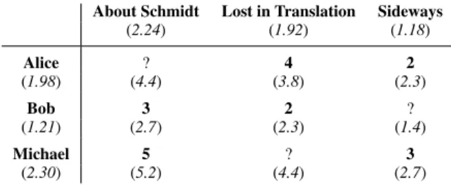
Figure 1: A simple latent-factor model for predicting movie ratings. (Data points in boldface, latent factors and estimated ratings in italics.)

fits naturally as a powerful abstraction for large factors while pro-gramming in Sparkler, and (b) the optimization opportunities in DSGD-based factorizations and how Sparkler takes advantage of them. Using several experiments, we demonstrate in Section 5 that Sparkler can offer 4x to 21x better performance for matrix factoriza-tion over Spark. The related work is discussed in Secfactoriza-tion 6 and we conclude in Section 7 and point to future work.

2. BACKGROUND

In this section, we provide a brief background on how the recom-mendation problem is modeled as a matrix factorization problem. We summarize existing results on how distributed stochastic gra-dient descent (DSGD) can be applied to this problem. Then we introduce Spark.

2.1 Low-rank Matrix Factorizations

As an instructive example, we consider the matrix completion problem that recommender systems need to solve. This task was central to the winning Netflix competition [20] as well as the latest KDD’11 cup. The goal of the recommendation problem is to provide accurate personalized recommendations for each individual user, rather than global recommendations based on coarse segments.

Consider the data depicted in Figure 1, which shows the ratings of three customers and three movies in matrix form. The ratings are printed in boldface and vary between 1 (hated the movie) and 5 (loved it). For example, Michael gave a rating of 5 to the movie “About Schmidt” and a rating of 3 to “Sideways”. In general, the ratings matrix is very sparse; most customers have rated only a small set of movies. The italicized number below each customer and movie name is alatent factor. In this example, there is just one factor per entity: Michael is assigned factor 2.30, the movie “About Schmidt” gets 2.24. In this simple example, the estimated rating for a particular customer and movie is given by the product of the corresponding customer and movie factors. For example, Michael’s rating of “About Schmidt” is approximated by2.30·2.24≈5.2; the approximation is printed in italic face below the respective rating. The main purpose of the latent factors, however, is topredictratings, via the same mechanism. Our estimate for Michael’s rating of “Lost in Translation” is2.30·1.92≈4.4. Thus, our recommender system would suggest this movie to Michael but, in contrast, would avoid suggesting “Sideways” to Bob, because the predicted rating is1.21·

1.18≈1.4. In actual recommender systems, the factor associated with each customer and movie is a vector, and the estimated rating is given by the dot product of the corresponding vectors.

More formally, given a largem×ninput matrixV and a small rankr, our goal is to find anm×rfactor matrixW and anr×n

factor matrixHsuch that V ≈ W H. The quality of such an approximation is described in terms of an application-dependent

(3)

loss functionL, i.e., we seek to findargmin_W_,_HL(V,W,H). For example, matrix factorizations used in the context of recom-mender systems are based on thenonzero squared lossLNZSL =

P

i,j:Vij6=0(Vij−[W H]ij) 2

and usually incorporate regulariza-tion terms, user and movie biases, time drifts, and implicit feedback. A very interesting class of loss functions is that ofdecomposable lossesthat, likeLNZSL, can be decomposed into a sum oflocal lossesover (a subset of) the entries inVij. I.e., loss functions that can be written as

L= X

(i,j)∈Z

l(Vij,Wi∗,H∗j) (1)

for sometraining setZ⊆ {1,2, . . . , m} × {1,2, . . . , n}and lo-cal loss functionl, whereAi∗andA∗jdenote rowiand columnjof matrixA, respectively. Many loss functions used in practice—such as squared loss, generalized Kullback-Leibler divergence (GKL), andLpregularization— belong in this class [34]. Note that a given loss functionLcan potentially be decomposed in multiple ways. For brevity and clarity of exposition we focus primarily on the class of noisy matrix completion, in whichZ={(i, j) :Vij6= 0}. Such decompositions naturally arise when zeros represent missing data as in the case of recommender systems. The techniques described here can handle other decompositions (like robust matrix factorization) as well; see [14, 15].

2.2 Distributed Stochastic Gradient Descent

for Matrix Factorization

Stochastic Gradient Descent(SGD) has been applied successfully to the problem of low-rank matrix factorization (the Netflix con-test [20] as well as the recent KDD’11 cup).

The goal of SGD is to find the valueθ∗∈ <k

(k≥1) that mini-mizes a given lossL(θ). The algorithm makes use of noisy observa-tionsLˆ0(θ)ofL0(θ), the function’s gradient with respect toθ. Start-ing with some initial valueθ0, SGD refines the parameter value by iterating the stochastic difference equationθn+1=θn−nLˆ0(θn), wherendenotes the step number and{n}is a sequence of decreas-ing step sizes. Since−L0(θn)is the direction of steepest descent, SGD constitutes a noisy version of gradient descent. To apply SGD to matrix factorization, we setθ = (W,H)and decompose the lossLas in (1) for an appropriate training setZ and local loss functionl. Denote byLz(θ) =Lij(θ) =l(Vij,Wi∗,H∗j)the local loss at positionz= (i, j). ThenL0(θ) =P

zL

0

z(θ)by the sum rule for differentiation. We obtain a noisy gradient estimate by scaling upjust oneof the local gradients, i.e.,Lˆ0(θ) =N L0z(θ), whereN =|Z|and the training pointzis chosen randomly from the training set.

We summarize the results from [15] on how to efficiently dis-tribute and parallelize SGD for matrix factorizations. In general, distributing SGD is hard because the individual steps depend on each other: The parameter value ofθnhas to be known beforeθn+1

can be computed. However, in the case of matrix factorization, the SGD process has some structure that one can exploit.

DEFINITION 1. Two training pointsz1, z2∈Zare interchange-ablewith respect to a loss functionLhaving summation form(1)if for allθ∈H, and >0,

L0z1(θ) =L 0 z1(θ−L 0 z2(θ)) and L0z2(θ) =L 0 z2(θ−L 0 z1(θ)). (2) Two disjoint sets of training pointsZ1, Z2⊂Zare interchangeable with respect toLifz1andz2are interchangeable for everyz1∈Z1

andz2∈Z2. Z11_Z12_Z13 Z21_Z22_Z23 Z31_Z32_Z33 Z11_Z12_Z13 Z21_Z22_Z23 Z31_Z32_Z33 Z11_Z12_Z13 Z21_Z22_Z23 Z31_Z32_Z33 Z11_Z12_Z13 Z21_Z22_Z23 Z31_Z32_Z33 Z11_Z12_Z13 Z21_Z22_Z23 Z31_Z32_Z33 Z11_Z12_Z13 Z21_Z22_Z23 Z31_Z32_Z33 Z1 Z2 Z3 Z4 Z5 Z6

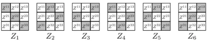
Figure 2: Strata for a3×3blocking of matrixV

For matrix factorization, two training pointsz1 = (i1, j1) ∈ Z

andz2 = (i2, j2)∈Zare interchangeable with respect to any loss functionLhaving form (1) if they share neither row nor column, i.e.,i16=i2andj16=j2. It follows that if two blocks ofV share neither rows or columns, then the sets of training points contained in these blocks are interchangeable.

The key idea of Distributed Stochastic Gradient Descent (DSGD) is that we can swap the order of consecutive SGD steps that involve interchangeable training points without affecting the final outcome. This allows us to run SGD in parallel on any set of interchange-able sets of training points. DSGD thus partitions the training set

Zinto a set of potentially overlapping “strata”Z1, . . . , Zs, where each stratum consists ofdinterchangeable subsets ofZ. See Fig-ure 2 for an example. The strata mustcoverthe training set in that Sq

s=1Zs=Z, but overlapping strata are allowed. The parallelism

parameterdis chosen to be greater than or equal to the number of available processing tasks.

There are many ways to stratify the training set into interchange-able strata. Onedata-independent blocking that works well in practice, is to first randomly permute the rows and columns of

V, and then created×dblocks of size(m/d)×(n/d)each; the factor matrices W andH are blocked conformingly. This procedure ensures that the expected number of training points in each of the blocks is the same, namely,N/d2. Then, for a per-mutationj1, j2, . . . , jdof1,2, . . . , d, we can define a stratum as

Zs=Z1j1∪Z2j2∪ · · · ∪Zdjd, where thesubstratumZijdenotes the set of training points that fall within blockVij. In general, the setSof possible strata containsd!elements, one for each possible permutation of1,2, . . . , d. Note that there is no need to materialize these strata: They are constructed on-the-fly by processing only the respective blocks ofV.

Algorithm 1 shows matrix factorization using DSGD. The indi-vidual steps in DSGD are grouped intosubepochs, each of which amounts to (1) selecting one of the strata and (2) running SGD (in parallel) on the selected stratum. Anepochis defined as a sequence ofdsubepochs. An epoch roughly corresponds to processing the entire data set once.

Algorithm 1DSGD for Matrix Factorization Require: V,W0,H0, cluster sized

BlockV /W/Hintod×d/d×1/1×dblocks

whilenot convergeddo /* epoch */

Pick step size

fors= 1, . . . , ddo /* subepoch */

Pickdblocks{V1j1_{, . . . ,}_Vdjd_}_{to form a stratum}

forb= 1, . . . , ddo /* in parallel */

Read blocksVbjb_,_Wb_and_Hjb

Run SGD on the training points inVbjb_{(step size}₌₎

Write blocksWb_and_Hjb

end for end for end while

2.3 Spark Background

Spark is a cluster computing framework aimed at iterative work-loads. Spark is built using Scala, a language that combines many

(4)

1 val lines = sc . textFile ("foo.txt")

2 val lower_lines = lines . map(String . toLowerCase _ )

3 val count_acc = sc . accumulator (0)

4 val prefix_brd = sc . broadcast (PREFIX)

5 lower_lines . foreach (s =>

6 if ( s . startsWith ( prefix_brd . value ) )

7 count_acc += 1

8 )

9 println ("The count is "+ count_acc.value)

Listing 1: Sample Spark code: accumulators and broadcast vari-ables.

features from functional programming as well as object oriented programming. Spark allows programmers to take the functional programming paradigm and apply it on large clusters by providing a fault-tolerant implementation of distributed in-memory data sets called Resilient Distributed Data (RDD). An RDD may be construct-ed by reading a file from a distributconstruct-ed filesystem and loading it into the distributed memory of the cluster. An RDD contains immutable data. While it cannot be modified, a new RDD can be constructed by transforming an existing RDD.

The Spark runtime consists of a coordinator node and worker n-odes. An RDD is partitioned and distributed across the workers. The coordinator keeps track of how to re-construct any partition of the RDD should one of the workers fail. The coordinator accomplishes this by keeping track of the sequence of transformations that led to the construction of the RDD (the lineage) and the original data source (the files on the distributed filesystem). Coordinator failures cannot be recovered from – the cluster needs to be restarted and the processing has be to relaunched.

Computation is expressed using functional programming prim-itives. For instance, assume that we have a set of strings stored in a file, and that the task at hand is to transform each string to lower case. Consider the first two lines of Spark code in Listing 1. The first line loads a set of strings from “foo.txt” into an RDD called lines. In the second line, themapmethod passes each string in linesthrough the functionString.toLowerCasein parallel on the workers and creates a new RDD that contains the lower-case string of each string inlines.

Spark additionally provides two abstractions – broadcast variables and accumulators. Broadcast variables are immutable variables, initialized at the coordinator node. At the start of any parallel RDD operation (like map or foreach), they are made available at all the worker nodes by using a suitable mechanism to broadcast the data. Typically, Spark uses a topology-aware network-efficient broadcast algorithm to disseminate the data. Line 4 in Listing 1 initializes a broadcast variable calledprefix_brdto some string called PREFIX. In Line 6, this value is used inside theforeachloop to check if any of the lines in the RDD calledlinesbegin with the string inprefix_brd.

An accumulator is a variable that is initialized on the coordinator node and is sent to all the worker nodes when a parallel operation (like map or foreach) on the RDD begins. Unlike a broadcast vari-able, an accumulator is mutable and can be used as a device to gather the results of computations at worker nodes. The code that executes on the worker nodes may update the state of the accumu-lator (for computations such as count, sum, etc.) through a limited update()call. At the end of the RDD parallel operation, each worker node sends its updated accumulator back to the coordinator node, where the accumulators are combined (using either a default or user-supplied combine function) to produce a final result. This result may either be output, or be used as an input to the next RDD parallel operation in the script. Example accumulator usages include sum, count, and even average.

We show an example of using accumulators and broadcast vari-ables by extending our last example. Suppose that the task is to count the number of strings with a given case-insensitive prefix. Listing 1 shows the Spark code for this problem. An accumulator is created as the counter and sent to all worker nodes, initialized to zero (Line 3). The prefix is broadcast to all worker nodes in Line 4. For each string inlower_lines, Line 6 updates the local counter associated with the accumulator on the worker. Finally, all the local counters are implicitly transmitted to the coordinator and summed up, after the parallel RDD operation onlower_linescompletes.

3. DSGD USING SPARK

In this section, we present how DSGD can be implemented using Spark, and point out the shortcomings of Spark.

Using plain Spark to factorize a large matrix requires maintaining a copy of the latent factor matrices on the nodes that update them. Under this constraint the DSGD algorithm can be expressed in Spark using existing abstractions, as depicted in Listing 2. The data is first parsed and partitioned (Line 9). The partitioning is done by assigning each rating tuple a row block ID and a column block ID, each between0andn, wherenis the number of strata. The block IDs are assigned using a hash function followed by a

modnto deal with skew in the input rating tuples. Each block of tuples is now grouped and assigned to a stratum. The output, strata, is a set of RDDs. Each RDD consists of the blocks of the corresponding stratum, and each block is simply a set of rating tuples. The partitioning function of the RDDs is overridden so that two properties are guaranteed: (1) The blocks of a stratum are spread out over the cluster in an RDD, and can be processed in parallel on different worker nodes; (2) The rating tuples in a given block are on exactly one worker node. All the above logic is packed into method DSGD.prepare.

The factor matrices (movieFactorsanduserFactors) are created on the coordinator node and registered with Spark as the accumulatorsmovieModelanduserModel(Lines 12 and 13). This information allows Spark to make the accumulator variable available at each of the worker nodes. The strata are processed one at a time (the blocks of each stratum are processed in parallel in Lines 16 – 23) in separate Spark workers. This inner loop is executed simultaneously at each worker node which processes a block of the stratum and updates the corresponding entries in the factor matrices. Since stratification guarantees that the updates on each worker will be to disjoint parts of the factor matrices, at the end of the job, the coordinator gathers all the updated values of the accumulators from the workers and simply concatenates them (there is no aggregation happening). The updated values ofmovieModel anduserModelare then sent out to the worker nodes for the next stratum. Once all the strata are processed, a similar set of jobs is used to compute the current error (Lines 26 – 32). The computation stops when the error drops below a pre-specified threshold or if a maximum number of iterations is reached.

A slight variant of this approach is to use broadcast variables to disseminate the factor matrices at the start of each subepoch. Broad-cast variables are distributed to the cluster using a more efficient mechanism than the coordinator simply copying the data structure over to each worker. This can be done with minor changes to the program, and is not shown here for brevity.

Spark’s existing abstractions for the factor matrices – such as accumulators and broadcast variables – perform poorly when the factors get larger. This is because of two reasons – first, Spark makes the assumption that these data structures are small enough to fit in the main memory of a single node. Second, even if this constraint is met, accumulators and broadcast variables are disseminated to

(5)

1 case class RatingTuple(movieId: Int , userId : Int , rating : Int ,...) 2 object RatingTuple {

3 def parse ( line : String ) = {...}

4 ...

5 }

6 ...

7 val data = sc . textFile ( inputFile )

8 val strata = DSGD.prepare(data, RatingTuple . parse )

9 varmovieFactors = FVector(rank)

10 var userFactors = FVector(rank)

11 varmovieModel = spark.accumulator(movieFactors )( FVector . Accum)

12 varuserModel = spark . accumulator( userFactors )( FVector . Accum)

13 do{

14 for ( stratum <−strata ) {

15 for (block <−stratum; x<−block) {

16 val ma = movieModel(x.movieId)

17 val ua = userModel(x. userId )

18 val d = ma∗ua−x. rating

19 val ufactor = realStepSize ∗(−d)∗2

20 ma.update(ua , ufactor )

21 ua. update(ma , ufactor )

22 }

23 }

24 var error = spark . accumulator (0.0)

27 // similar code to calculate error

28 // and update realStepSize

29 ...

30 }

31 }

32 iterationCount ++

33 }while ( error > targetError && iterationCount < iterationLimit )

Listing 2: Factorization in Spark using accumulators. the entire cluster from the coordinator node and the updated ver-sions are gathered back before merging. This is unnecessary in the context of DSGD matrix factorization since each worker node only works on a small and disjoint portion of the factor matrices. This makes communication a very significant part of the overall time for the factorization task. Figure 3 illustrates this point by plotting the execution time of a single iteration of thedo..whileloop in List-ing 2 (usList-ing broadcast variables) as the rank of the factor matrices increases. The Netflix dataset was used on a 10-node cluster. The details of the dataset are in Section 5.

As is evident from the figure, for a given dataset size, as the rank increases, the runtime for each iteration also rapidly increases. Us-ing factor matrices of rank 200 – 400 is not uncommon for complex recommendation problems. In fact, the winners of the Netflix Chal-lenge [20] and KDD’11 cup report using factors of approximately this size. As the rank and the dataset grow, the broadcast-based approach no longer works since the factors do not entirely fit in memory.

4. DSGD USING SPARKLER

To address the above deficiencies, we present Sparkler, a parallel platform built on Spark that is tailored for Matrix Factorization. Sparkler introduces (a) a novel distributed memory abstraction for large factors called Carousel Map that provide a major performance advantage over using accumulators and broadcast variables, and (b) several optimizations that take advantage of the computation and communication patterns during DSGD factorization.

4.1 Carousel Map (CM)

At a high level, a CM is a distributed hash table where only a portion of the table is stored on each node. Thus using a CM, the aggregate memory of the entire cluster can be used to store the factor

Rank 0 50 ₁₀₀ ₁₅₀ ₂₀₀ ₂₅₀ ₃₀₀ ₃₅₀ ₄₀₀ Time (sec) 0 500 1000 1500 2000 2500 3000 _Spark

Figure 3: Execution time of a single epoch on a 10-node cluster, on the Netflix dataset using Spark as the rank of the factor matrices increases.

matrices. A CM can retrieve the factors vector given a key (movieID or a userID) in constant time by looking up the routing information for a given key and retrieving the value from the appropriate node. However, this only overcomes the first problem of fitting the factor matrices in the aggregate memory of the cluster.

Lookups/updates are a frequently executed operation in a factor-ization. They constitute the main inner computational loop at the workers as shown in Lines 17 – 22 in Listing 2. As a result, making them efficient is critical to getting good performance. We exploit the nature of the DSGD algorithm to ensure that the CM is partitioned and stored in such a way thatmostof the lookups and updates hap-pen locally. In fact, the data structure is designed to live in the same process (JVM) as the worker node, and as a result a lookup does not even incur inter-process communication (IPC) overheads. This is of critical importance since an in-process hash table lookup can be substantially faster than an out-of-process lookup using IPC, and orders of magnitude faster than incurring network I/O and looking this up using remote procedure calls.

The CM is accessed in a way that does not require the coordinator to be involved in either gathering data to combine updates, nor disseminating the data to the workers. The CM is initialized in a distributed fashion on the worker nodes; and at the end of subepochs, the worker nodes directly exchange data. Finally, the data structure is garbage collected when it is no longer needed. The coordinator never sees any of the actual data and is eliminated from being the bottleneck. These techniques allow the developer to use CMs to scale to recommendation problems on substantially larger datasets as well as use larger ranks for the factors than is currently possible with Spark. Equally importantly, CMs are included in Sparkler as a natural extension that does not require major changes on the part of the programmer. Listing 3 shows how the Spark program from Listing 2 can be modified to use CMs by only changing 2 lines (Lines 12 – 13).

4.2 CM API

The CM is used simply as amapof keys to values. It supports two functions :get(key)andput(key, value). In a typical DSGD program, keys can be the IDs for the data items (movieID, userID), and the values are the factor vectors corresponding to the items. The CM is also registered with an initialization function – initialize(key)which returns a suitable initial value for a feature vector if it isn’t present in the map. This allows the data structure to be initialized across the worker nodes as necessary

(6)

7 ...

8 val data = sc . textFile ( inputFile )

9 val strata = DSGD.prepare(data, RatingTuple . parse )

10 varmovieFactors = FVector(rank)

11 var userFactors = FVector(rank)

12 varmovieModel = spark.CM(movieFactors)(FVector.Accum)

13 varuserModel = spark.CM(userFactors)(FVector.Accum)

14 do{

17 ...

Listing 3: Modifications required for factorization in Sparkler using CMs. A1 A2 B1 B2 A3 B3 C1 C2 C3 Users 1 2 3 A B C M ovi e s U₁ U₂ U₃ M_A MB M_C X

Figure 4: Strata blocks.

instead of initializing it in its entirety on the coordinator node.

4.3 CM Data Movement

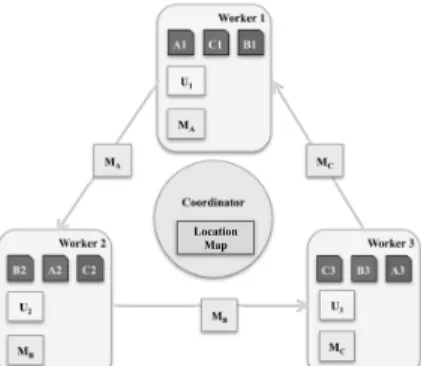
The intuition behind how nearly all accesses to the CM can be ser-viced locally is best explained using an example. Consider Figure 4 which shows a matrix of users and movies stratified into a 3x3 grid. For simplicity, assume this matrix is to be factorized on a cluster of 3 nodes. The first stratum consists of blocks labeled A1, B2, and C3; the second stratum consists of blocks labeled A2, B3, and C1; and finally, the third stratum consists of blocks labeled A3, B1, and C2. Note that the Users and Movies factor matrices are partitioned correspondingly to U1, U2, U3and MA, MB, MC.

Consider the subepoch where the first stratum consisting of blocks A1, B2, and C3 is processed. The data is already laid out so that each of these blocks is on a different node on the cluster. When the SGD computations begin, the node processing A1 (sayworker1) needs to read and write the entries for the movies and users corresponding to partitions A and 1 (MAand U1). In this subepoch,worker1will

not need to access any other partitions of the factor matrices. In the same subepoch,worker2processes B2, and therefore only accesses partitions U2and MB. No two nodes access or update the same

entries in either the customer or movie model in a given subepoch. In the next subepoch, blocks A2, B3, and C1 are processed. These blocks are onworker2,worker3, andworker1respectively.worker1 now requires access to factor partition U1 and MC. Since in the

previous subepoch this worker was updating partition U1, it already

has this data locally. It now needs access to partition MC. To locate this, it first contacts the coordinator node, which replies that this partition is onworker3. Then, it directly contactsworker3and requests that it bulk transfers the movie factor partition MC; we refer to such an operation as atransfer of ownership. The actual data transfer happens directly betweenworker3andworker1without involving the controller node. The entire MCpartition is moved over, not just the key being requested. Figure 5 shows the transfers that take place at the start of the second subepoch. Once this transfer

Worker 1 MA U1 Worker 2 Worker 3 Coordinator MB U2 MC U3 B1 A1 C1 C2 B2 A2 C3 B3 A3 MA MB MC Location Map

Figure 5: CM communication pattern.

is done, all the accesses the factor matrices in this subepoch are done locally. As Figure 5 shows, the partitions of a factor move in a circle after each subepoch, hence the name “Carousel Map”.

4.4 CM Implementation

The CM is implemented in two parts. When a CM is created, it is registered at the Spark coordinator. The coordinator node maintains a location table for each CM, which maps each partition of the CM to a worker node. This node is marked as theownerof the partition. Simple hash-based partitioning is used to divide the key-space into the required number of partitions. The same hash function needs to be used to partition the input matrix as well as the factor matrices. This ensures that any CM partition contains data for items from at most one partition of the matrix, and will therefore be accessed from exactly one worker during any given subepoch. The worker nodes store the data corresponding to each CM partition in a simple hash table.

Algorithm 2 describes the logic that is executed whenget()is invoked on a CM on one of the workers. The worker first checks to see if it is the current owner of the partition that contains the requested key. If it is, then it fulfills the request by looking up the local hash table. Otherwise, it requests the coordinator for the address of the current owner of this partition. Having located the owner, it requests a transfer of ownership from the current owner to itself. This involves serializing and moving the hash table from the current owner to the requesting node and re-constituting it so it can be accessed. Theget()call blocks until the partition is moved to the requesting node. Once the transfer completes, the coordinator is updated with the new owner. A similar protocol is used forput() requests.

Once the node gets ownership of a partition, theget()function (or theput()function) can be locally executed. Since the CM partition is stored in the same JVM in which the program logic is executing, further accesses to the CM partition are equivalent to local lookups in a hash table and do not require any IPC or remote I/O.

The major advantage of using CMs over accumulators or broad-cast variables is in saving network costs. For large factorization problems, the factor matrices can be tens of gigabytes. Accumula-tors in Spark need to be sent from the coordinator node to all the worker nodes at the start of a parallel job. At the end, the mod-ified accumulator values need to be gathered from each worker node and combined at the coordinator to arrive at the correct val-ue for the accumulator. Similarly, broadcast variables also need to be sent out from the coordinator to each of the worker nodes. Broadcast variables are not updated, and need not be collected and combined like accumulators. As one would guess from these ab-stractions, a naive implementation would quickly make the network

(7)

interface card of the controller node a major bottleneck in imple-menting accumulators and broadcast variables. With large clusters, sending out the model data from the coordinator and gathering it back quickly becomes the dominant portion of the time spent in factorizing. Efficient implementations, such as the ones described recently [7], use network-topology-aware broadcast protocols. Simi-lar in-network reduction techniques can be used while gathering the updated accumulators for combining. The CM is a data placement and communication abstraction that is aware of the accesses it is going to receive. As a result, it can be far more efficient than a simple accumulator or a broadcast variable.

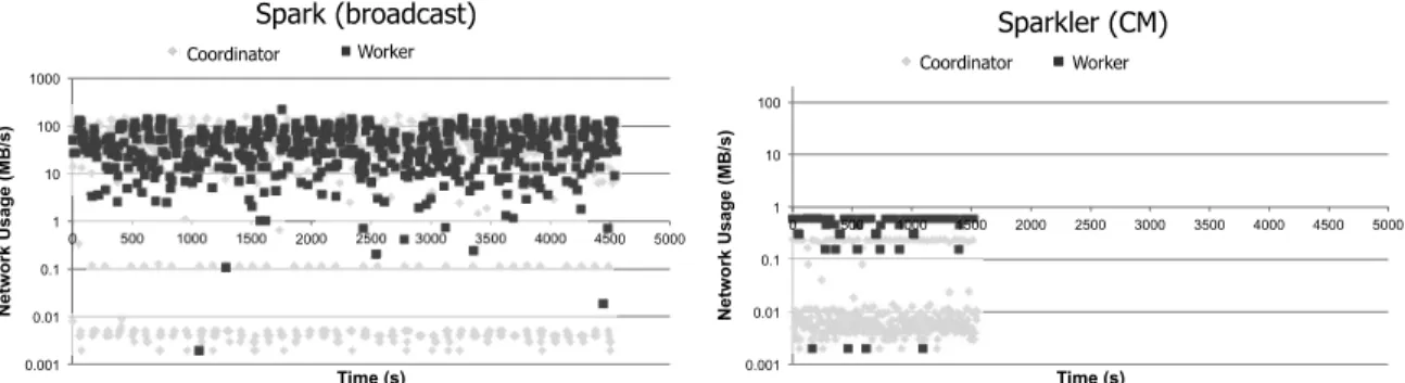
As a quick sanity test, we show the result of a simple experiment that measured the network traffic at the coordinator node and the worker nodes during a factorization run. In Figure 6, the left half shows the network traffic when the job was run with plain Spark, and the right half when the job was run with Sparkler and CMs. The dataset used was the Netflix dataset [20], on a cluster of 40 nodes, using factor matrices of rank 400. The total traffic in the first scenario was 167GB and 143GB at the controller and worker nodes respectively. With CMs, this is reduced to 55MB and 126MB respectively over a similar timeframe. This dramatic reduction in communication is largely responsible for the performance advan-tages we will explore in detail in Section 5.

Algorithm 2Worker Algorithm for CM get() Require: A keyk, CMM, the worker nodew

Letpid= partition ID corresponding tok

ifpidis owned bywthen

return pid.get(k)

else

ohost= current owner ofpidfrom coordinator

request ownership transfer forpidfromohosttow

associatepidwith the received hash table

return pid.get(k)

end if

4.5 CM Fault-Tolerance

RDDs (Resilient Distributed Datasets) in Spark provide lineage-based fault-tolerance. In case of failure, any partition of RDDs can be reconstructed from the initial data source or the parent RDDs. However, the fault-tolerance mechanism of RDDs is inefficient for CMs. First, in contrast to coarse-grained transformations in RDDs, CMs support fine-grained updates as required in the DSGD algorithm. Second, CMs are designed for iterative algorithms. A lost partition of a CM may contain updates accumulated over hundreds of iterations. Due to both reasons, lineage-based fault-tolerance becomes overwhelmingly expensive. As a result, we chose a simple fault-tolerance mechanism – periodic checkpointing.

A CM can be checkpointed by simply invoking acheckpoint() function. When this function is invoked, the Sparkler coordinator sends a checkpoint request to all the nodes that own at least one partition of the CM along with a version number. Each node writes this partition of the CM, along with the version number to the distributed filesystem. This is a blocking checkpoint algorithm. The next job is started only after all the nodes have finished check-pointing and the coordinator has received acknowledgments from all of them. CMs also support arecoverFromCheckPoint ()function. When this is invoked, the current state in the CM is discarded, and the last known complete checkpoint of the CM is loaded in from the distributed filesystem.

During the course of a job, if one of the worker nodes fails, the coordinator instructs all the nodes to discard the current version of the CM and load the last known complete checkpoint from the DFS.

13 ...

14 do{

15 try {

16 for ( stratum <−pData. strata ) {

18 val ma = movieModel(x.movieId)

19 val ua = userModel(x. userId )

20 val d = ma∗ua−x. rating

21 val ufactor = realStepSize ∗(−d)∗2

22 ma.update(ua , ufactor )

23 ua. update(ma , ufactor )

24 } 25 } 26 movieModel.checkpoint() 27 userModel.checkpoint() 28 } catch (LostCMNode l) { 29 movieModel.recoverFromCheckPoint() 30 userModel.recoverFromCheckPoint() 31 } 32 ...

Listing 4: Fault-tolerance for CMs through checkpoints. If any job is in progress, an exception (of typeLostCMNode) is thrown. The user can catch this exception, and recover from it using therecoverFromCheckPoint()function, and simply resume computation. Since this is user-managed checkpointing, it requires some minor modifications to the code. Listing 4 shows a snippet of the program from Listing 3 enhanced with checkpoint and recovery code. As is evident from the figure, it only requires a simple, minor change to incorporate fault-tolerance. In the future, we plan to allow Sparkler to automatically pick the checkpoint frequency based on the failure characteristics expected from the cluster.

4.6 Sparkler Optimizations

In this section we describe two optimization choices that Sparkler automatically performs without requiring any manual user interven-tion.

4.6.1 Sparkler Data layout

The choice of the precise strategy used for laying out the strata of the matrix across the nodes of the cluster can impact the total amount of network traffic that is incurred during factorization. Re-call that after each subepoch, when a new stratum is being processed, each worker node needs to fetch the partitions of the factor matrices corresponding to the data block that it is working on. With a care-fully designed data layout, it is possible to ensure that the worker nodes only need to fetch one of the two factor matrix partitions from a remote node and that the other factor matrix can remain local across subepochs. This serves to further decrease the overall communication costs for factorization.

We first provide a brief calculation for the amount of data ex-changed between subepochs to ensure that the factor matrices are available locally during the data processing step. Consider a dataset overMmovies andU users containingDdata points. Assuming that the factor matrices have a rankr, and they store the features as

4-byte floating point numbers, the movie matrix is of size4×r×M

and the user matrix is of size4×r×U. Assume that the cluster consists ofnnodes. If we partition the data inton strata, each worker stores4×r_n×M and4×r_n×U bytes of data for the factor trices. At the end of each stratum, in general, both the factor ma-trix partitions need to be fetched from a remote node, leading to

n×(4×r_n×M +4×r_n×U)bytes to be transferred over the network in total before each stratum is processed. For an iteration over alln

strata, this results in4nr(M+U)bytes of network traffic. Consider a layout where each worker node contains all the data for

(8)

!"!!#$ !"!#$ !"#$ #$ #!$ #!!$ #!!!$ !$ %!!$ #!!!$ #%!!$ &!!!$ &%!!$ '!!!$ '%!!$ (!!!$ (%!!$ %!!!$ ! " #$ % &' () * + , " (-./ 0* 1( 234"(-*1( )*+,-$./+01$23-403**50$!""#$%&'("#) )*+,-$./+01$+$.*+65$7,8/!&9$*"#+,#) -.'#+)/0#"'$1'2(3) !"!!#$ !"!#$ !"#$ #$ #!$ #!!$ !$ %!!$ #!!!$ #%!!$ &!!!$ &%!!$ '!!!$ '%!!$ (!!!$ (%!!$ %!!!$ ! " #$ % &' () * + , " (-./ 0* 1( 234"(-*1( ./+01::$23-403**50$!""#$%&'("#) ./+01::$+$.*+65$7,8/!&9$*"#+,#) -.'#+4,#)/!53)

Figure 6: Network traffic at coordinator and workers: comparison between broadcast variables and CMs. a given user partition. For example, in the scenario of Figure 4, data

blocks A1, B1, and C1, each belonging to a different stratum are co-located on the same worker node. With this layout, when switching from one subepoch to another, a given worker node will only need to fetch a partition of the movie factor matrix from a remote node since the next user factor matrix partitions corresponding to the data on the worker node (partition 1) is already local. Choosing A1, B1, C1 to be the data blocks on the worker node ensures that the data processing only ever requires a single partition of the factor matrix on that worker. With this data layout, the total amount of network traffic can be reduced to4nrM bytes if only the movie factor partitions are moved around. Alternatively, if the data is partitioned by the movie dimension, the total traffic is4nrUbytes. The above presents us with an optimization opportunity in choos-ing the appropriate data layout to minimize data transfers between subepochs. In the Netflix example,M is of the order of 100,000 whileU is of the order of a few million. As a result, it makes more sense to choose the layout that results in4nrMbytes of network traffic. In the preparation phase, one can easily determine which is the larger dimension by using several known techniques [3]. This is one of the optimization choices that is made by Sparkler.

4.6.2 Sparkler Partitioning

The granularity of partitioning of the input matrix determines the number of strata and therefore the number of Spark jobs that are required to complete one iteration over the data. Since each job incurs a non-trivial initialization overhead, choosing the granularity of partitioning has a major effect on the execution time. If a small number of partitions are used, there may not be enough memory on each node to hold the partition of the data as well as the corre-sponding factor matrix partitions. On the other hand, if too many partitions are made, it will require a larger number of (shorter) jobs – one for each subepoch. Sparkler uses a simple formula to pick the right number of nodes using as input the size of the dataset, the rank of the factorization, the available memory on each node, and the number of nodes available.

If the aggregate memory available in the cluster is less than that required to efficiently complete the problem, the model is kept in memory, and the partitions of the RDD are paged into memory when required. This ensures that the data structures that can be accessed sequentially are read from disk while those that need random ac-cess are pinned in main memory. Experiments in Section 5 show the effect of varying the partitioning granularity on the execution time for each iteration. Section 5.3 measures the impact of these optimization choices on the overall execution time.

5. EXPERIMENTS

In this section, we present the results of several experiments that

explore the advantages of using Sparkler and CMs over Spark and its existing abstractions of accumulators and broadcast variables. We also explore the performance impact of the optimization choices that Sparkler makes.

The experiments were run on a 42-node cluster connected by a 1Gbit ethernet switch. Each node has two quad-core Intel Xeon processors with 32GB of main memory and five 500GB SATA disks. One node was reserved to run the Mesos [17] master and the HDFS (Hadoop Distributed File System) Namenode. Another node was reserved to run the Spark coordinator. The remaining 40 nodes were available for use as workers for Spark. The software versions used were IBM’s J9 JVM for Java 1.6.0, HDFS 0.20.2 from Hadoop, and Scala 2.8.1, and Spark version 0.3.

The experiments used the dataset from the Netflix prize [20]. The dataset has 100,198,805 ratings for 480,189 users and 17,770 items. To generate larger instances of the problem, we doubled the dataset along both dimensions to create a dataset that was four times as large, and another one that was sixteen times as large. As in previous papers [15], this approach was used to synthetically obtain larger datasets while retaining the same sparsity as the original dataset. The datasets are referred to as N1, N4, and N16 in this section.

5.1 Comparison with Spark

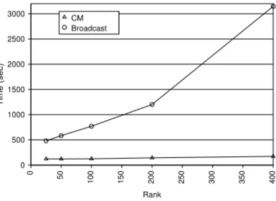
The first set of experiments focus on the advantage of using CMs when compared to the existing abstractions of accumulators and broadcast variables in Spark. Figure 7a shows the time taken for a single epoch over the dataset on a cluster of size 5 as the rank of the factor matrices is increased for the Netflix dataset (N1). As described in Section 2.2, completing the actual factorization is likely to take several epochs. As in previous work [15], we focus on the time taken in a single iteration to directly compare performance without any interference from randomness and convergence rates. As the rank is varied from 25 to 400, the execution time for Sparkler with CMs varies from 96 seconds to 193 seconds. On the other hand, the time for Spark using broadcast variables varies from 594 seconds to 2,480 seconds. Sparkler is 6.2x - 12.9x faster. As is evident, CM’s advantage gets larger as the rank of the factors gets larger. This is because Spark needs to broadcast as well as accumulate a larger amount of model data as the rank gets larger. CM avoids the cost of transferring all this data over the network and therefore scales much better. The experiment was repeated on a 10-node cluster with similar results: CM was 3.9x to 18.3x faster (Figure 7b).

Figures 8a and 8b compare the execution time per epoch of CMs and broadcast variables for a fixed rank, 50, and vary the data size. The times are shown for N1, N4, and N16. Note that the Y-axis is on a logarithmic scale. On the 5-node cluster, CM’s advantage over broadcast for N1 and N2 were 6.3x and 9.2x respectively. For N16, broadcast didn’t finish even after 15,000 seconds, and was terminated. The factor size increases linearly with both the

(9)

Rank 0 50 ₁₀₀ ₁₅₀ ₂₀₀ ₂₅₀ ₃₀₀ ₃₅₀ ₄₀₀ Time (sec) 0 500 1000 1500 2000 2500 3000 _CM Broadcast

(a) cluster size = 5

Rank 0 50 ₁₀₀ ₁₅₀ ₂₀₀ ₂₅₀ ₃₀₀ ₃₅₀ ₄₀₀ Time (sec) 0 500 1000 1500 2000 2500 3000 _CM Broadcast (b) cluster size = 10 Figure 7: Using CMs vs broadcast variables as rank increases

Data Size N1 N4 _N16 Time (sec) 50 150 350 750 1550 3150 6400 _CM Broadcast

Data Size N1 N4 _N16 Time (sec) 50 150 350 750 1550 3150 6400 _CM Broadcast (b) cluster size = 10 Figure 8: Using CMs vs broadcast variables as data size increases

number of items and the number of customers. As a result, the broadcast based approach is much worse for larger datasets. On the 10-node cluster CM was 5x, 9.4x, and 21x faster on N1, N4, and N16 respectively (Figure 8b).

5.2 Scaling Results

Next, we studied the performance of CMs as we varied the rank at different dataset sizes for different cluster sizes. Figure 9a shows the time taken per epoch as the rank of the factor matrices is increased for N1 and N4 on a cluster of 5 nodes. N16 was too large for the 5 node cluster and is not shown. Figures 9b and 10a show the same experiment on clusters of size 10 and 20 respectively. For a given cluster size, CMs scale linearly with increasing rank so long as the CM can fit in aggregate memory. We expect that CMs will work with arbitrarily large ranks as long as the aggregate memory of the cluster is large enough. This is in contrast to accumulators and broadcast variables that need to fit in the main memory of a single node or use B-trees, both of which are major bottlenecks. We note that this holds for all the cluster sizes shown here: 5, 10, and 20.

5.3 Optimizations

Next we study the contribution of the optimization choices to improving the runtime of each epoch. Recall that Sparkler chooses the data layout in a way that allows the larger factor (say customers) to stay resident on the same worker across subepochs while forcing

Params Optimal (sec) Reversed (sec) Ratio

Dataset=N1, 5 nodes Rank 25 95.8 104.5 1.1x 50 117.9 114.7 1.0x 100 113.8 135.2 1.2x 200 144.1 181.6 1.3x 400 192.7 258.5 1.3x Dataset=N1, 10 nodes Rank 25 121.9 123.4 1.0x 50 120.7 128.9 1.1x 100 124 145.9 1.2x 200 143 173.4 1.2x 400 172.3 236.9 1.4x

Table 1: Impact on execution time for choosing the larger stable dimension.

the smaller factor’s CM to move its partitions around from subepoch to subepoch. Table 1 shows execution time per epoch when the larger factor is kept stable as well as when this is reversed. As is expected, the penalty for choosing the wrong dimension to be stable increases with the rank of the factorization, and varies from nearly no penalty when the rank is small (25) to 1.4x when the rank is large (400).

(10)

Rank 0 ₅₀ 100 150 200 250 300 350 400 Time (sec) 0 500 1000 1500 2000 2500 N1 N4

Rank 0 ₅₀ 100 150 200 250 300 350 400 Time (sec) 0 500 1000 1500 2000 2500 N1 N4 N16 (b) cluster size = 10 Figure 9: Factorization Time as rank increases

Rank 0 50 ₁₀₀ ₁₅₀ ₂₀₀ ₂₅₀ ₃₀₀ ₃₅₀ ₄₀₀ Time (sec) 0 500 1000 1500 2000 2500 N1 N4 N16

(a) Factorization Time as rank increases, cluster size = 20

Cluster Size 0 5 ₁₀ ₁₅ ₂₀ ₂₅ ₃₀ ₃₅ ₄₀ Time (sec) 150 200 250 300 350 400 450 N4

(b) Execution Time as cluster size increases Figure 10

The second choice Sparkler makes that could have an important impact on the execution time is the size of the cluster used. Because each epoch is split into as many subepochs as there are strata, there are substantial overheads to stratifying the matrix to be processed over more nodes. Figure 10b shows the execution time per epoch for varying choices of cluster size on the N4 dataset with rank=50. The best execution time is obtained at a cluster size of 10. As clusters larger than 10 are used, the overhead of partitioning the data into strata, and the fixed per-job overheads start to dominate. Between cluster sizes of 5 and 40, the ratio of the worst time to the best time was about 2x.

Sparkler uses a simple model based on data size, rank, available memory, and computation and communication costs to pick the right sized cluster. This can easily be overridden by the user who wishes to explicitly instruct Sparkler to use a given number of nodes.

6. RELATED WORK

Sparkler draws on ideas from several different research commu-nities, and builds on a growing body of work dealing with efficient algorithms and systems for solving learning tasks on very large data sets.

There has been much research in the past on the general goal of being able to support existing shared-memory applications trans-parently on distributed system [13]. CMs offer a different kind of

shared memory abstraction that does allow fine-grained updates so long as the updates are temporally and spatially correlated. Our approach with CMs is much more focused and limited than distribut-ed shardistribut-ed memory (DSM). Previous approaches to implementing DSM on clusters have met with little success because it is a difficult problem to provide this abstraction and have applications written for a single machine seamlessly work well without any modifications on DSM.

Several research groups have proposed alternatives to conven-tional MapReduce implementations for iterative workloads. Apart from Spark, these include Piccolo [29], HaLoop [5], Twister [11], Hyracs [4] and Nephele [2]. Since DSGD iterates over large datasets multiple times, these systems are of particular interest. The ideas in this paper can be adapted to work with any of these platforms.

Piccolo [29] advocates distributed in-memory tables as a program-ming model for cluster computation. Such a model is a lower-level abstraction than MapReduce. Given user-defined locality prefer-ence, Piccolo minimizes remote access by co-locating partitions of different tables that are more likely to be accessed by the same node. Piccolo also supports user-managed checkpointing for efficiently programming large clusters for data intensive tasks. Fault-tolerance in CMs draws on ideas similar to checkpointing in Piccolo. Howev-er, instead of presenting a general table abstraction, Sparkler uses RDDs for the data (with transparent fault tolerance), and CMs for

(11)

the factors (with user-managed checkpointing). Moreover, Piccolo adopts a fixed co-location scheme, while CMs provides a mecha-nism of dynamic collocation to further reduce remote access when possible.

HaLoop [5] proposes several modifications to Hadoop to improve the performance of iterative MapReduce workloads. However, Spark has shown that for iterative workloads, especially where the dataset fits in the aggregate memory of a cluster it offers substantially better performance [41] than Hadoop and HaLoop.

Twister [11] is an independently developed lightweight Map-Reduce runtime that is also optimized for iterative workloads. Twister also targets cases where the data fits in the aggregate memory of a cluster. However it does not support fault tolerance either for the input data or the data structures that store the factors. Hyracks [4] is a distributed platform designed to run data-intensive computations on large shared-nothing clusters of computers. Hyracks expresses computations as DAGs of data operators and connectors. Operators operate on partitions of input data and produce partitions of output data, while connectors repartition operators’ outputs to make the newly produced partitions available at the consuming operators.

Nephele [2] is a system for massively parallel data processing based on the concept of Parallelization Contracts(PACTs). PACT programs are compiled, optimized, and parallel executed on the Nephele execution engine performing various complex data analyti-cal tasks.

We chose Spark because the RDD abstraction is a great fit for many problems. Also, Spark is versatile and has been used to ex-press many data-parallel processing frameworks [41] including Map-Reduce, Bulk Synchronous Parallel for graph processing, HaLoop [5] and even a simple subset of SQL. Further, it is implemented in Scala – its conciseness makes it easy to express DSGD algorithms, the embedded DSL (Domain Specific Language) features [31] allow us to transparently make optimization choices, and the functional features make it easier for us to efficiently execute DSGD algorithm-s. While traditional parallel programming frameworks like MPI (Message Passing Interface) allow for very high performance and flexibility, it is difficult to provide two major advantages that Spark provides: fault-tolerance and ease-of-programming. We believe that that Spark and CMs offer the right combination of fault-tolerance, ease-of-programming, and adequate performance to be widely use-ful.

SystemML [16] is a project that aims to build a language for expressing machine learning algorithms and a compiler and runtime that executes them as a series of MapReduce jobs on Hadoop. Sys-temML is general-purpose – it is not focused on iterative workloads or on datasets that fit in memory. In contrast, Sparkler focuses on iterative learning tasks on datasets that fit in the aggregate memory of a cluster. Sparkler offers much higher performance for such cases than a general-purpose platform.

A closely related work is the Victor [12] project at the University of Wisconsin. Victor attempts to bring together the techniques re-quired for expressing stochastic gradient descent algorithms on data in large relational databases using User Defined Functions (UDFs) and a simple python interface. We believe that this approach will be extremely valuable in making SGD-style algorithms accessible on large relational datasets. Finally, parallel and distributed algorithms (including DSGD variants) for large-scale matrix completion on problems with millions of rows, millions of columns, and billions of revealed entries are discussed in [39]. The focus is on main-memory algorithms that run on a small cluster of commodity nodes using MPI for computation. However, Sparkler targets alternate architectures. Much like Spark, our design is aimed at being able

to solve this problem on a large cluster of machines and does not require the data to be in a relational database. Furthermore, unlike relational databases where mechanisms like UDFs typically impose a performance penalty as well as development overheads, our design is aimed to support development of DSGD algorithms through a lightweight domain specific language tailored for this task. Finally, unlike parallel relational databases or MPI clusters, Sparkler (and Spark) are particularly well-suited to running on the cloud.

There are other systems specialized for matrix computations. MadLINQ [30] provides a programming interface for distributed matrix computations based on linear algebra. A MadLINQ program is translated into a DAG of parallel operators, and the output of each operator is pipelined to downstream operators. This approach is similar to using Hadoop, and does not exploit efficient memory sharing in the cloud. Presto [40] is a prototype that supports R running on a cluster. Presto extends R language for distributed execution, and supports efficient update of the results when the input matrices are incrementally changed. Presto partitions the matrices, and co-locates the partitions operated by the same function. A partition can be read by multiple concurrent tasks form different nodes, but written only by the owner node. However, Presto does not allow changing the ownership of partitions to further reduce remote access as in CMs.

On the surface, CMs are also related to research in scalable dis-tributed hash tables (DHTs) motivated by peer-to-peer internet ap-plications. Chord [37] and Pastry [32] are well known examples of such systems. These systems focus on providing efficient, fault-tolerant routing at internet-scale under the assumption that members may arbitrarily join and leave the system. In contrast, CMs are de-signed to support access to large factors, specifically in the context of DSGD programs. Unlike DHTs, CMs do not focus on problems of churn, membership protocols, and routing.

A naive alternative to using CMs is to use a distributed cache such as Memcached [25]. However, using Memcached as a simple key-value store to hold the model data presents two problems: first, each access to the hashmap will in general require network I/O to reach the node that contains the data. Second, memcached does not provide any fault-tolerance if a node fails. CMs solve both these problems without imposing an undue burden on the programmer.

Hogwild! [27] is a recent result that shows how multi-threaded SGD algorithms can be implemented without using locks to serialize updates to the shared model. This is a particularly interesting result with substantial performance advantages, we plan to use this in our multithreaded version to obtain similar speedups.

There’s a rich history of work on several different algorithms for personalized recommendation and collaborative filtering [38]. In this paper, we do not propose any new algorithms for recommen-dation. Instead, we focus on building a platform to support a class of algorithms (SGD) that has been shown to be very promising for solving general matrix factorization problems.

There has also been recent work in the database community to increase the flexibility with which a recommendation engine can be used to display actual results to the user [21]. The techniques in this work address a single-node shared-everything database, and are not focused on scaling out to solve large instances of the problem. Other aspects of this work that address flexibility in incorporating additional constraints are complementary to Sparkler and CMs, and are generally useful for any practical recommender system.

7. CONCLUSIONS AND FUTURE WORK

We view Sparkler as not merely a tailored solution to a “narrow” problem of matrix factorization using DSGD. As others have pointed out [36], matrix factorization is no longer just for matrix