FaMIDAS: A Mixed Frequency Factor Model with MIDAS structure

Temi di Discussione

(Working Papers)

FaMIDAS:

a

m

ixed

f

requency

f

actor

m

odel

with MIDAS structure

by Cecilia Frale and Libero Monteforte

788

uar

y 20

Temi di discussione

(Working papers)

FaMIDAS:

a

m

ixed

f

requency

f

actor

m

odel

with MIDAS structure

by Cecilia Frale and Libero Monteforte

The purpose of the Temi di discussione series is to promote the circulation of working papers prepared within the Bank of Italy or presented in Bank seminars by outside economists with the aim of stimulating comments and suggestions.

The views expressed in the articles are those of the authors and do not involve the responsibility of the Bank.

Editorial Board: MARCELLO PERICOLI, SILVIA MAGRI, LUISA CARPINELLI, EMANUELA CIAPANNA, DANIELA MARCONI, ANDREA NERI, MARZIA ROMANELLI, CONCETTA RONDINELLI, TIZIANO ROPELE, ANDREA SILVESTRINI.

FAMIDAS: A MIXED FREQUENCY FACTOR MODEL WITH MIDAS STRUCTURE

by Cecilia Frale* and Libero Monteforte**

Abstract

In this paper a dynamic factor model with mixed frequency is proposed (FaMIDAS), where the past observations of high frequency indicators are used following the MIDAS approach. This structure is able to represent with richer dynamics the information content of the economic indicators and produces smoothed factors and forecasts.

In addition, the Kalman filter is applied, which is particularly suited for dealing with unbalanced data set and revisions in the preliminary data. In the empirical application for the Italian quarterly GDP the short-term forecasting performance is evaluated against other mixed frequency models in a pseudo-real time experiment, also allowing for pooled forecast from factor models.

JEL Classification: E32, E37, C53.

Keywords: mixed frequency models, dynamic factor models, MIDAS, forecasting.

Contents

1. Introduction... 5

2. The Model... 7

2.1 The factor model with mixed frequency ... 7

2.2 The MIDAS for the lags combination ... 8

2.3 The FaMIDAS ... 10

3. The empirical application ... 11

4. Forecasting evaluation... . 13

5. Conclusions ... 15

Appendix: The State space representation and temporal aggregation... 17

References ... 19

Tables and figures... 22

_______________________________________

* MEF-Ministry of the Economy and Finance-Italy, Treasury Department.

1

Introduction*

The impact of the recent financial crisis on the real economy was underestimated by a num-ber of forecasters. Both academia and policymakers are now thinking about the ability of macroeconometric models to make predictions about the economy and identify early signals of turning points. In practice, short-term forecasting mainly relies on two sets of instruments: bridge models and factor models. Bridge models link timely indicators with low frequency target variables, whereas factor models extract a common component from a set (usually large) of series1. In their standard formulation, bridge and factor models have shown some limitations with respect to two major topics: the time aggregation bias and the ragged-edge data problem, which is a relevant issue for real time forecasts.2

Recently, there has been an increase in research papers on these two approaches with ex-tensions in different directions, including mixed frequency models which represent a promis-ing field of research. Mixed frequency models are particularly useful for extractpromis-ing the in-formation content from high frequency indicators that are used as proxies for target variables observed at lower frequency and with a time lag. Given that this is what economic forecast-ers do in their day to day work, these models are of particular interest to them. Moreover, these models provide a tool for time series disaggregation, given that the target variable is estimated at a higher frequency.

The mixed frequency literature was initially developed using state space factor models, estimated via the Kalman filter. Most of the applications exploit monthly series, such as industrial production or confidence surveys, to predict quarterly GDP. This approach was used by Mariano and Murasawa (2003), Mittnik and Zadrozny (2004), Proietti and Moauro (2006), Aruoba et al. (2009), Camacho and Perez Quiros (2009) and Frale et al. (2010a). These models can also be used as a multivariate tool for time series disaggregation, as done in Frale et al. (2010b), Harvey and Chung (2000), Moauro and Savio (2005).

*This paper represents the authors personal opinions and does not reflect the view of the Bank of Italy and the Italian Department of Treasury. We are grateful to participants in the 3rd CFE-Cyprus 2009, especially to Ana Galv˜ao and Gianluca Moretti for helpful comments and conversations. We benefit from the discussion during the MIDAS Workshop, Frankfurt 2010, and in particular we would like to thank Eric Ghysels, Massi-miliano Marcellino and Rossen Valkanov for useful advices. We received additional advices during the 30th CIRET Conference in New York and from Jules Leichter. Routines are coded in Ox 3.3 by Doornik (2001) and are based on the programs realized by Tommaso Proietti for the Eurostat project on EuroMIND: the Monthly Indicator of Economic Activity in the Euro Area.

1_{On the comparison of the different models for short term predictions see Barhoumi, Benk, Cristadoro,} Reijer, Jakaitiene, Jelonek, Rua, R¨unstler, Ruth and Nieuwenhuyze (2009).

2_{The problem of the unbalanced data set in large scale factor models has been tackled with different} so-lutions in Altissimo et al. (2007) and Marcellino and Schumacher (2010). On time aggregation bias see Marcellino (1999).

A different approach relates to the recent literature on Mixed Data Sampling Regression Models (MIDAS) proposed by Ghysels, Santa-Clara and Valkanov (2002, 2006). MIDAS mainly differ from mixed frequency factor models as they are univariate, with lag polynomi-als being used to combine high frequency indicators with the low frequency target variable. There is a small, but fast growing, literature on MIDAS models. Most of the early appli-cations refer to financial econometrics, but there have recently been a number of papers on GDP and inflation. Clements and Galv˜ao (2010) and Andreu et al. (2008) suggest a MI-DAS to forecast US macro variables on a monthly and daily basis. Monteforte and Moretti (2010) propose a MIDAS to predict monthly inflation on a daily basis in real time. Mar-cellino and Schumacher (2010) use a MIDAS to deal with an unbalanced large data-set and for predicting the GDP by means of monthly factors.

In this paper we combine the two approaches and we propose a state space factor model with mixed frequency, where the past observations of high frequency indicators follow a MIDAS structure. This feature is new in the literature and enables the exploitation, in a parsimonious way, of a larger number of lags of the high frequency indicators. This is par-ticularly useful in forecasting as it explicitly takes into account the cross correlation between indicators and the target variable. Moreover, the MIDAS polynomial produces smooth fac-tors, which is a desirable property as it implies less volatile forecasts. This is a relevant issue especially for policy analysis and turns out to be quite important in periods of high variabil-ity of macroeconomic data, such as during economic crises. Our approach of combining factor models and MIDAS regression complements the one of Marcellino and Schumacher (2010). They propose a large scale mixed frequency factor model where monthly factors are aggregated to quarterly by using a MIDAS structure, while we proposes a small scale model where the mixed frequency is in the state space and the MIDAS component is only used to consider more lags of the indicators.

The combination of mixed frequency and MIDAS structure allow matching two different and relevant issues: having a monthly index for business cycle analysis, like for dating the cycle and mitigate the noise effect of preliminary data in real time applications. In the empir-ical application with Italian data, the predictive performance of the Mixed Frequency Factor MIDAS (FaMIDAS in the following) is compared with a multivariate (VAR) model, a mixed frequency univariate model (ADL) and with two mixed-frequency factor models (with single and multiple factors). The results seem to suggest that the FaMIDAS prevails at larger hori-zons in real time forecasting. This is not surprising, as the factor produced by FaMIDAS is smooth and thus less affected by the short-run variability of the data. The next Section gives an overview of the model, while Section 3 deals with estimation and data issues. Section 4 reports the results of the forecasting exercise and Section 5 draws conclusions.

2

The Model

This section presents the main model of the paper. The aim of this new approach is to increase the flexibility of factor models and thus to improve their ability to reproduce the underlying structural model of economic agents in a framework that is essentially a reduced form. As a matter of fact factor models are pure statistical models, with lack of economic interpretation. Therefore, including a richer dynamics as we do by using a MIDAS structure may be also seen as an indirect way to capture the behavior of economic agents. An example of this would be the expectation formation process, which might induce changes over time in the correlation among time series.

A complementary approach has been followed by Marcellino and Schumacher (2010), where they combine factors and MIDAS in a different structure. In particular we extract a monthly factor using MIDAS polynomial on each indicator, while they adopt a MIDAS structure to project monthly factors for quarterly forecasts. In the following the two main ingredients of the model, and the way in which they are integrated, are presented.

2.1

The factor model with mixed frequency

There are many possible ways of linking a set of indicators available at high frequency to the target variable observed at shorter time intervals.

In particular, we start from a dynamic factor model that decomposes a vector of N time se-ries,y𝑡, with different frequencies (e.g. monthly and quarterly), into one (or more) common

nonstationary components, 𝑓𝑡, and some idiosyncratics,𝛾𝑡, specific to each series. Both the

common factor and the idiosyncratic components follow autoregressive standard processes as shown by the following representation:

y𝑡 = 𝝑0𝑓𝑡+𝝑1𝑓𝑡−1 +𝜸𝑡+S𝑡𝜷, 𝑡= 1, ..., 𝑛,

𝜙(𝐿)Δ𝑓𝑡 = 𝜂𝑡, 𝜂𝑡 ∼NID(0, 𝜎𝜂2),

D(𝐿)Δ𝜸_𝑡 = 𝜹+𝜼∗

𝑡, 𝜼∗𝑡 ∼NID(0,Σ𝜂∗),

(1)

where𝜙(𝐿)is an autoregressive polynomial of order𝑝with stationary roots and D(𝐿)is a diagonal matrix containing autoregressive polynomials of order 𝑝𝑖 (i=1 to N) . The vector

𝛿 contains the drifts of the idyosincratic components. The regression matrix S𝑡 contains

the values of exogenous variables that are used to incorporate calendar effects (trading day regressors, Easter, length of the month, etc.) and intervention variables (level shifts, additive outliers, etc.), and the elements of 𝜷 that are used for initialisation and other fixed effects. The disturbances𝜂𝑡and𝜼∗𝑡 are mutually uncorrelated at all leads and lags.

autoregressive process of order p,𝜙(𝐿)−1_𝜂

𝑖𝑡an individual𝐴𝑅(𝑝𝑖)process,𝑑𝑖(𝐿)−1𝜂∗𝑖𝑡and a

mean term𝛿𝑖, The error terms,𝜂𝑖𝑡and𝜂𝑖𝑡∗ are difference stationary and independent.

Variables are considered in level as common in the unobservable components approach and the cointegration is rouled out on purpose as extensively argumented in Frale et Alt. (2010b). The model is cast in a linear State Space Form (SSF) and, assuming that the dis-turbances have a Gaussian distribution, the unknown parameters are estimated by maximum likelihood, using the prediction error decomposition, performed by the Kalman filter.

The SSF is suitably modified to take into account the mixed frequency nature of the series. Following Harvey (1989), the state vector is augmented by an ad hoc cumulator function which translates the problem of aggregation in time into a problem of missing values. The cumulator is defined as the observed aggregated series at the end of the season (e.g. last month of quarter), otherwise it contains the partial cumulative sum of the disaggregated values ( e.g. months) making up the aggregation interval (e.g. quarters) up to and including the current one. The model might include a procedure for expressing volumes in chain link prices and therefore allows matching the monthly estimates with national account identities published by national statistical offices.

Given the multivariate nature of the model and the mixed frequency constraint, the maxi-mum likelihood estimation can be numerically complex. Therefore, the univariate filter and smoother for multivariate models proposed by Koopman and Durbin (2000) is used as it pro-vides a very flexible and convenient device for handling high dimension data sets and missing values. The main idea is that columns in the matrix y𝑡, 𝑡 = 1, . . . , 𝑛are stacked on top of

one another to yield a univariate time series whose elements are processed sequentially.

2.2

The MIDAS for the lags combination

As is well known in the literature of leading indicators, the anticipating power of an eco-nomic series for any target variable is purely an empirical concept. Even more cumbersome is the case of mixed frequency data, where the indicators are available at higher frequency with respect to the target, so that not even autocorrelation analysis is helpful. Consider, for example, that we want to use a well-know leading indicator such as the Business Climate or Purchase Manager Index (PMI) to have a preliminary assessment of the state of the econ-omy before the release of GDP, which is observed on average two month after the end of a quarter. Although it is well know that such indicators have a leading power, we do not know exactly the leading power (in terms of quarters) of the monthly PMI. Even more, we might prefer a more flexible model, so that the leading order can change over time. In our view, a more efficient and suitable solution to this issue is the application of MIxed DAta Sampling models (MIDAS) which summarize and combine the information content of the

indicators and their lags with weights jointly estimated. Usually the treatment of mixed data sample is solved by first aggregating the highest frequency in order to reduce all data to the same frequency and then, in a second step, estimating a regression. This implies imposing some restrictions on the parameters of the aggregating polynomial and does not exploit all the information available. The MIDAS models overcome this problem as they exploit full information without imposing any restrictions on the parameters that are estimated jointly. Some restrictions could be introduced to reduce the parameter space and avoid the cost of parameter proliferation.

MIDAS models have recently encountered considerable success due to their simplicity and good performance in empirical applications. To introduce them, as in the seminal paper by Ghysels et al. (2002, 2006), suppose𝑌𝑡is a time series variable observed at a certain fixed

frequency and let𝑋𝑚_{be an indicator variable sampled m times faster. A MIDAS regression}

takes the form:

𝑌𝑡=𝛽0+𝐵(𝜃, 𝐿1/𝑚)𝑋𝑡𝑚+𝜖𝑡

where𝐵(𝜃, 𝐿1/𝑚_{) =}∑𝐾

𝑘=0𝑏(𝜃, 𝑘)𝐿𝑘/𝑚is a polynomial of length K and𝐿1/𝑚is an operator

such that 𝐿𝑘/𝑚_𝑋𝑚

𝑡 = 𝑋𝑡𝑚−𝑘/𝑚. In other words the regression equation is a projection of 𝑌𝑡

into a higher frequency series𝑋𝑚

𝑡 up to k lags back.

The MIDAS structure mainly involves two elements: the reconciliation of different fre-quency and the use of lagged values of the indicators.

In our application, the MIDAS component is only used in order to include in a parsi-monious structure past values of indicators, whereas the time aggregation problem is solved inside the factor model as shown in Section 2.1. This allows better interpretation of the cycli-cal pattern of the economic indicators and comparability with benchmark dynamic models.

Regarding the weight structure, two main possibilities have been proposed in the litera-ture. First, a parametrization that refers to Almon lags:

𝑏(𝑘;𝜃) = 𝑒𝑥𝑝(𝜃1𝑘+...𝜃𝑞𝑘

𝑞₎

∑𝑘

𝑗=1𝑒𝑥𝑝(𝜃1𝑘+...𝜃𝑞𝑘𝑞)

.

Second, weights drawn by a Beta distribution, such as:

𝑏(𝑘;𝜃1, 𝜃2) = 𝑓(𝑘;𝜃1, 𝜃2) ∑𝑘 𝑗=1𝑓(𝑘;𝜃1, 𝜃2) where𝑓(𝑥, 𝑎, 𝑏) = 𝑥𝑎−_𝐵1(1_(𝑎,𝑏−𝑥₎)𝑏−1,𝐵(𝑎, 𝑏) = Γ(_Γ(𝑎_𝑎)Γ(_+𝑏𝑏₎) andΓ(𝑎) =∫∞ 0 𝑒(−𝑥)𝑥𝑎 −1_𝑑𝑥.

There is no clear a priori reason for preferring one parametrization over another, and the choice should clearly depend on the research problem under analysis. It should be noted

that, as a rule of thumb, the Beta function, given its flexibility, seems more suitable when the number of lags considered is large, whereas the simplicity of the Almon weights might be preferable in the case of a small number of time lags.

Looking at the recent literature, Marcellino and Schumacher (2010) used the Almon weights for the estimation of GDP in real time, whereas Monteforte and Moretti (2010) found the Beta transformation more appropriate for the estimation of inflation which involves daily data and more than 20 lags.

2.3

The FaMIDAS

This section presents how to combine the dynamic factor model with mixed frequency and the MIDAS structure of lags described in the previous section.

Starting from the model in equation (1) let us partitioning the set of time series, y_𝑡, into two groups,y𝑡= [y1′,𝑡,y2′,𝑡]′, where the second block represents the target variable available

at lower frequency and the first part is a MIDAS structure based on high frequency indicators

xtso thaty₁′_,𝑡= [𝑏(𝐿_𝑘, 𝜃)xt]′.

The FaMIDAS follows from the following equations:

[ 𝑏(𝐿𝑘, 𝜃)xt y2,𝑡 ] = 𝝑0𝑓𝑡+𝜸𝑡+S𝑡𝜷, 𝑡= 1, ..., 𝑛, 𝜙(𝐿)Δ𝑓𝑡 = 𝜂𝑡, 𝜂𝑡 ∼NID(0, 𝜎𝜂2), D(𝐿)Δ𝜸_𝑡 = 𝜹+𝜼∗ 𝑡, 𝜼∗𝑡 ∼NID(0,Σ𝜂∗), (2)

Model 2 collapse to model 1 if K=0 and𝜗=0. In our application𝑏(𝐿𝑘, 𝜃)is the exponential

Almon lag polynomial:∑𝐾

𝑘=0𝑤(𝑘, 𝜃)𝐿𝑘with 𝑤(𝑘, 𝜃) = 𝑒𝑥𝑝(𝜃1𝑘+𝜃2𝑘 2₎ ∑𝐾 𝑘=0𝑒𝑥𝑝(𝜃1𝑘+𝜃2𝑘2) .

Actually this formalization represents a parsimonious way of including in the model lagged values for the common factor.

The dynamic factor model is estimated by specifying an AR(2) process for the common component and the idiosyncratic components of the monthly indicators in difference. For GDP, the idiosyncratic component is formulated as a random walk with drift. This restricted specification is motivated by the fact that there are identification problems of the kind that have been discussed by Proietti (2006) with reference to the Litterman model, which affect the estimation of autoregressive effects.

For the MIDAS polynomial the weights sum up to 1 so that their size is fully comparable. As far as the maximum lag length is concerned, the target horizon of forecasting and the

economic meaning of the series could suggest the appropriate number. One can consider alternatively to include the lagged values of indicators in the matrix𝑦𝑡without the MIDAS

restriction. This approach, not only has a cost in terms of degree of freedom, as the number of parameters to be estimated would increase considerably, but it fails to consider the time series dimension of lagged values. In fact, without the MIDAS restriction lagged values of the indicators would be included in the model as part of different series.

The model is cast in State Space Form and the Maximum Likelihood estimates are ob-tained through suitable filtering procedures based on the Kalman filter prediction error de-composition. Starting from a trial for all parameters, including those in the MIDAS structure, the procedure is run iteratively so that the weights in the MIDAS maximize the Likelihood function associated with the factor model. The standard procedure documented in Frale et al. (2010b) is therefore modified adding the restrictions which link the hyperparameter𝜃1,2

to the parameters𝑤(𝑘, 𝜃).

In the empirical application we investigate the content of nowcasting and forecasting GDP each month in real time, exploiting the information coming from timely indicators of eco-nomic activity. We also discuss the performance of the FaMIDAS model compared to other mixed frequency model and to more standard formalizations. We show that the integrated approach used in our framework provides flexibility in working with data expressed at dif-ferent frequency, released with difdif-ferent delay and revised every time a new observation is published. Furthermore we stress how our model efficiently deals with dynamic cross corre-lation among indicators available at different frequencies.

3

The Empirical Application

The aim of the empirical application is to exploit the information of the most relevant monthly economic indicators, available earlier than the official statistics, to disaggregate, nowcast and forecast quarterly GDP. This is used to estimate the unobserved monthly GDP, both for the past (a monthly indicator of the known quarterly GDP) and for the future. It is worth noting that in this model the monthly indicator is fully consistent with the quar-terly data in terms of time aggregation. Thus we obtain an indicator that can be used both in sample as a monthly measure of GDP to date the cycle and out of sample as a leading indicator.

The GDP is estimated directly, leaving the bottom-up approach (estimation by aggrega-tion of sectoral value added or components of demand) for future research. Although the model is specified in levels in order to easily deal with the time constraint, the results and the forecasting experiment are presented in growth rates, which is the reference measure for

both policy makers and academics.

As for the variable selection, a wide set of indicators is considered, with series referring to different aspects of the economy. These are mainly national statistics data, such as industrial production; survey data, such as climate, expectations and PMI (Purchasing Manager Index); financial data, such as spreads and money (M2); and other data such as the CPB index of world trade, production of paper, electricity consumption and traffic flows of heavy goods vehicles. Although the information set has a small scale, the models incorporate a variety of properly chosen indicators referring to the real economy as well as finance, national and international, in the service and manufacturing sectors. Variables are taken directly from the source in seasonally adjusted values, except for electricity consumption and traffic of trucks which have been seasonally adjusted using the Tramo-Seats routine and smoothed when needed3_{. For the model selection process we follow the standard approach in the literature,}

based, for example, on statistical significance of the indicators and BIC or Akaike criteria for the lag length selection.

After some empirical robustness checks, the sample ranging from January 1990 up to the most recent observations at the time of writing (April 2009) was found to have the best trade-off among representativeness of the sample size, availability of long time series and data quality. Some benchmark models have been estimated.

The central model is our factor model with MIDAS structure (FaMIDAS), based on an information set with 4 indicators and combinations of up to 4 lags: Industrial production, German PMI, Business climate, Electricity consumption. Alternative lag lengths have been evaluated accordingly to a reasonable forecast horizon (maximum 6 months ahead) and the economic meaning of the indicators. We compare the empirical performance of our FaMI-DAS with two multivariate models.

Then we consider a baseline model (MIXFAC) specified as in equation (1) and based on the same information set than the FaMIDAS, but without MIDAS component and one lag of the first two series.

Finally we also estimate a factor model with 2 factors (MIX2FAC), as discussed in Frale et al. (2010a), which includes additional indicators: Industrial production of paper, world trade, Treasury Italian yields (10Y), Money supply, traffic flows of heavy goods vehicles.

The baseline MIXFAC model involves both survey and national account data. The MIX2FAC model includes more soft indicators and the second factor captures also financial swings, as they comes up ex-post. Finally, using FaMIDAS, it is possible to consider up to four lags of each economic indicator of MIXFAC.

The estimated maximum likelihood parameters are listed in Table 1, whereas the monthly

3_{No calendar effect neither intervention variables are included in the matrix𝑆}

indicators are shown in Figure 1. In addition, Figure 2 shows the estimated GDP in monthly growth rates and the common factors for the three models. The graph clearly shows that the FaMIDAS produces a smoother factor which is a desirable property, likely a product of the fact that the MIDAS structure sums over time lags. Similarly, the disaggregated monthly GDP from the FaMIDAS is more stable than the same obtained by the other two mixed frequency models (MIXFAC and MIX2FAC). Moreover, the confidence bands of the predic-tions, shown as fan charts in Figure 3, reveal smaller incertitude in the FaMIDAS model than in the other mix-frequency formulations.

The inspection of the spectral density of the estimated monthly GDP for the MIDAS and MIXFAC, shown in Figure 4, suggests that the FaMIDAS structure is able to capture standard business cycle frequencies and, therefore, might perform better in short-term forecasting than in nowcasting. Analyzing the minor volatility in terms of spectrum of frequencies, it turn out that the FaMIDAS picks up the less volatile components of the spectrum and thus the estimates are less affected by the noise of data revisions that occur in real time analysis. Indeed the fact that previsions from the FaMIDAS are less volatile makes them particularly useful for dealing with real time data which are subject to revision and, therefore, suffer for high degree of uncertainty.

The forecasting performance analysis of the three models requires an empirical applica-tion, which is presented in the next section. On the contrary, the production of a monthly measure of GDP which is a derivative of this framework is not the focus of this paper.

4

Forecasting evaluation

In this section the three models under analysis are compared with respect to their forecast-ing ability for the Italian GDP by usforecast-ing a rollforecast-ing experiment in a window of the latest 5,4 years up to the end of 2007 4_{. The rolling exercise is made in pseudo-real time, so as to}

mimic the delay of different indicators, which has been proved to be relevant for correctly assessing which model performs best. Therefore the forecasting evaluation is made with specification of the month of the prediction inside the quarter (e.g. first month, second or third), which corresponds to a different information set. It is worth stressing that the Kalman filter is particularly suitable for this issue given that it solves endogenously the problem of the unbalanced sample produced by the difference in timing of publication of the monthly indicators. Consider the example of making a forecast for GDP in the 1st of January 2011.

4_{We prefer to exclude the biennium 2008-2009 from the sample to avoid that the exceptional conditions of} the economic crisis affect the results. In addition, at the time of writing, data from 2008 upwards were still preliminary and subject to revision.

The last release of GDP refers to the third quarter of 2010 and thus before making forecast for one or two parters ahead, it is required to estimate the last quarter of GDP for 2010 which is still unknown. Analogously, monthly indicators are published with a certain delay. In January, for example, we would have soft indicators, such as PMI or Business climate, for December 2010, while Industrial production for November 2010 would be release around the 15 of January 2011. Therefore indicators need to be forecasted for closing the quarter that should be predicted so as to balance the sample.

The Kalman filter allows doing this step endogenously as it solves directly the ragged-edge data issue by using the prediction routine. Moreover, every time a new observation for an indicator is released, all the series are generally revised for prior years and the MIDAS component helps reducing the statistical noise of the revisions in real time.

In Table 2 we show RMSE of the three mixed frequency factor models and of two addi-tional benchmark models. To disentangle the contribution of the mixed frequency structure, we also consider a quarterly VAR (estimated with order 2 on the bases of the AIC criteria) that includes the same information set as the MIXFAC. Moreover, to assess the gain of the multivariate structure we consider a univariate ADL modified as in Proietti (2006) to repli-cate a mixed frequency structure. We also considered as benchmark a model similar to the Factor-MIDAS of Marcellino and Schumacher (2010), where the MIDAS structure is ap-plied to the common factors. Although the two authors use a large dataset of indicators, we constrained the information set to be coherent with the other models for sake of comparison. We see that all factor models easily outperform the other two benchmark models. Consider-ing, in particular, the three mixed frequency models, we see that the differences in predictive ability are small and the ranking changes with the sample, the forecasting horizon and the monthly information. The ranking is also subject to the loss function as it is slightly differ-ent in the RMSFE and MAPE. For the case of a linear specification we see (Table 3) that the absolute value of the forecast errors are almost always smaller for the FaMIDAS in𝑄𝑡+1and

𝑄𝑡+2. Looking jointly at RMSE and MAPE, it seems that the MIX2FAC is more suited for

nowcasting, FaMIDAS makes the lowest RMSE for one quarter-ahead and Factor-MIDAS tends to prevail for two quarters ahead.

More generally, given the apparent absence of clear dominance of one model, we per-formed the DMW tests (Diebold and Mariano(1995) and West (1996)) of equal forecast ability to check if the ranking showed by RMSE is statistically significant. In particular, we tested the hypothesis that FaMIDAS has the same predictive information as the other two models. The results, in Table 4, are coherent we the evidence shown in the previous table: MIX2FAC dominates for 1-step ahead predictions, whereas FaMIDAS tends to make the smallest error for 2-step ahead forecasts, respect to all models including the Factor-MIDAS.

Since the seminal paper by Bates and Granger (1969), it is well know that combining different models results in a smaller forecast error than selecting a single specification. The general idea is that the combination of different specifications, by averaging, mitigate the model misspecification, instability and estimation error of each specific model (Timmermann 2006). Therefore, the pooling forecast is particularly suitable when the combined models show significant heterogeneity.

The application presented above matches this requirement, given that the models differ in terms of components (number of factors and lags), as well as for the best forecast horizon. In the bottom panel of Table 2 and Table 3 we report the real time errors for the pooled model with equal weights5_{. The combination of the three models, the MIXFAC, MIX2FAC and}

FaMIDAS appears useful in real time, as the error size is always close to those of the best model.

In fact, the forecasts produced by the pooling of different models dominates the single models more often for the RMSE than for the MAPE. A more proper combination would require a dedicated analysis that we leave for future research.

To summarize, we find that the mixed frequency factor models outperform standard VAR and univariate mixed frequency ADL. The differences in the forecasting ability of the three factor models are small, time dependent and not always statistically significant. In general, it emerges that MIXFAC and MIX2FAC appear more suited for nowcasting, while FaMIDAS and Factor-MIDAS seem better for forecasting. Northwitstanding the small differences in RMSE a forecast combination of the three factor models reduces further the error, likely thanks to the heterogeneity in the structure of the three models.

5

Conclusions

The short-term forecasting literature has shown an increasing interest in mixed frequency models. These models are particularly useful in real time forecasting as they deal with the unbalanced data set problem and they reduce the temporal aggregation bias created by the different frequencies of the observable indicators. In this paper we combine two approaches: dynamic mixed frequency factor models and MIDAS. Our model, that we call FaMIDAS, is designed for applications in real time as it reduces the problem of the unbalanced data set and it is less affected by revisions of preliminary data. Moreover it can take into account changes over time of the leading power of timely high frequency indicators used for forecasting.

As by product we obtain a monthly index of GDP which is per-se relevant for business

5_{Although the simple average of forecast is not optimal, under general circumstances and symmetric loss} functions it can generate a smaller loss (see Elliott and Timmermann (2004))

cycle analysis, as for example for defining a chronology of the cycle, application that we left for future research.

In the empirical application we estimate the FaMIDAS against benchmark models and mixed frequency factor models with different structures. Overall the FaMIDAS produces smoother estimates for the disaggregate target variable and better forecasts for one quarter ahead. In order to reduce further the prediction error a simple pooling forecasts is proposed.

Appendix: The State space representation and temporal

ag-gregation

Consider the factor model proposed in section 2.3:

y𝑡 = [ 𝑏(𝐿𝑘, 𝜃)xt y2,𝑡 ] = 𝝑0𝑓𝑡+𝜸𝑡+S𝑡𝜷, 𝑡= 1, ..., 𝑛, 𝜙(𝐿)Δ𝑓𝑡 = 𝜂𝑡, 𝜂𝑡 ∼NID(0, 𝜎𝜂2), D(𝐿)Δ𝜸_𝑡 = 𝜹+𝜼∗ 𝑡, 𝜼∗𝑡 ∼NID(0,Σ𝜂∗). (3)

where𝑏(𝐿𝑘, 𝜃)xtis the MIDAS polynomial for the combination of lags of the monthly

eco-nomic indicators andy2,𝑡is the aggregated variable that gathers the flow subject to temporal

aggregation ( e.g. the quarterly GDP). D(L) is a matrix containing autoregressive loading of the idyosincratics components. The common factor and the idiosyncratic components fol-low standard autoregressive processes and thus the model can be easily casted in State Space Form (SSF).

Consider the standard way to recast in SSF a general AR(𝑝) process𝜙(𝐿)Δ𝑓𝑡 =𝜂𝑡with

𝜙(𝐿) = (1−𝜙1𝐿−𝜙2𝐿2−...−𝜙𝑝𝐿𝑝): 𝑓𝑡=e′1,𝑝+1𝜶𝑡, 𝜶𝑡=Tf𝜶_𝑡−1+H𝜂_𝑡, where 𝜶𝑡= [ 𝑓𝑡 f∗ 𝑡 ] , Tf = [ 1 e′ 1𝑝T𝜙 0 T𝜙 ] ,T_𝜙 = ⎡ ⎢ ⎢ ⎢ ⎢ ⎣ 𝜙1 .. . 𝜙𝑝−1 I_𝑝−1 𝜙𝑝 0′ ⎤ ⎥ ⎥ ⎥ ⎥ ⎦ . andf_𝑡∗ =T𝜙f𝑡∗−1 +e1𝑝𝜂𝑡,H= [1,e′1,𝑝]′,e1𝑝 = [1,0, . . . ,0]′ .

And then apply the previous representation to the common factor and each idiosyncratic. The SSF of the complete model results:

y𝑡= [ 𝑏(𝐿𝑘, 𝜃)xt y2,𝑡 ] =Z𝜶𝑡+S𝑡𝜷, 𝜶𝑡=T𝜶𝑡−1+W𝒃+H𝝐𝑡, (4)

where the state vector and the vector of errors are obtained stacking the single SSF represen-tation of the autoregressive processes, namely:[𝛼𝑡 =𝛼𝑓,𝑡′ , 𝛼′𝛾1,𝑡, . . . , 𝛼

′

𝛾𝑁,𝑡]

′_{, for the state and} 𝝐𝑡= [𝜂𝑡, 𝜂1∗,𝑡, . . . , 𝜂∗𝑁,𝑡]′ for the vector of errors.

The system matrices of the measurement equation become:

Z = [ 𝜽0, ... 𝜽1 ... 0 ... diag(e′𝑝1, . . . ,e ′ 𝑝𝑁) ] , T=diag(T𝑓,T𝛾1, . . . ,T𝛾𝑁), H=diag(H𝑓,H𝛾1, . . . ,H𝛾𝑁). (5)

The matrixWis time invariant and selects the drift𝛿𝑖for the appropriate state element of

the idiosyncratic component.

The temporal aggregation problem is solved following the strategy proposed by Harvey (1989). The block of variables subject to temporal aggregation,y2, are replaced by an ad hoc

cumulator variable,y₂𝑐_,𝑡, defined so that it coincides with the (observed) aggregated series at the end of the larger interval (e.g. quarter), otherwise it contains the partial cumulative value of the aggregate in the seasons (e.g. months), as follow:

y₂𝑐_,𝑡 =𝜓𝑡y𝑐2,𝑡−1+y2,𝑡, 𝜓𝑡 =

{

0 𝑡=𝛿(𝜏 −1) + 1, 𝜏 = 1, . . . ,[𝑛/𝛿] 1 otherwise,

The cumulator is used to replace the second block of the measurement equation and to augment the state equation as follow:

𝜶∗_𝑡 = [ 𝜶𝑡 y₂𝑐_,𝑡 ] , y†_𝑡 = [ 𝑏(𝐿𝑘, 𝜃)xt y𝑐_2,𝑡 ]

The final measurement and transition equation are therefore:

y†_𝑡 =Z∗𝜶∗_𝑡 +S_𝑡𝜷, 𝜶∗_𝑡 =T∗𝜶∗_𝑡−1+W∗𝜷+H∗𝝐𝑡, (6)

with system matrices:

Z∗ = [ Z1 0 0 I𝑁2 ] , T∗ = [ T 0 Z2T 𝜓𝑡I ] , W∗ = [ W Z2W+S2 ] , H∗ = [ I Z2 ] H. (7)

References

Altissimo, F., Cristadoro , R., Forni M., Lippi M.,Veronese G. (2007). New Eurocoin: Tracking Economic Growth in real time, Bank of Italy working paper n. 631.

Andreou E., Ghysels E. , and A. Kourtellos, (2009), “Should macroeconomic forecasters use daily financial data and how?”, UNC Working Paper.

Aruoba, S. B., F. X. Diebold, and C. Scotti, (2009), “Real-time Measurement of Business Conditions”, Journal of Business & Economic Statistics 27 (4).

Barhoumi, K., S. Benk, R. Cristadoro, A. D. Reijer, A. Jakaitiene, P. Jelonek, A. Rua, G. R¨unstler, K. Ruth, and C. V. Nieuwenhuyze (2009). “Short-term forecasting of GDP using large monthly datasets: a pseudo real-time forecast evaluation exercise”, Journal of

Forecasting 28 (7).

Bates, J.M., C.W.J. Granger, (1969), “The combination of forecasts”, Operations Research

Quarterly 20.

Camacho, M., and G. Perez-Quiros, (2009), “Introducing the Euro-Sting: short term indi-cator of the Euro Area growth”, CEPR Discussion Paper No. 7343. Available at SSRN: http://ssrn.com/abstract=1461972

Clements, M. P., and A. B. Galv˜ao, (2010), “Real-time Forecasting of Inflation and Output growth in the Presence of data Revisions”, manuscript.

Diebold F., Mariano R.,(1995),“Comparing Predictive Accuracy”, Journal of Business and Economic Statistics, American Statistical Association, 13.

Doornik, J.A., (2001), Ox 3.0 - An Object-Oriented Matrix Programming Language, Tim-berlake Consultants Ltd: London.

Elliott, G., and Timmermann, A., (2004), “Optimal forecast combinations under general loss function and forecast error distribution”, Journal of Econometrics, Elsivier, vol. 122(1).

Frale, C., M. Marcellino, G. L. Mazzi, T. Proietti, (2010)a, “Survey data as Coincident or Leading Indicators”, Journal of Forecasting 29, special issue: dvances in Business Cycle Analysis and Forecasting, Jan-Mar 2010.

Frale, C., M. Marcellino, G. L. Mazzi, T. Proietti, (2010)b, “EUROMIND: A Monthly Indicator of the Euro Area Economic Conditions”, forthcoming in the Journal of the Royal Statistical Society series A.

Ghysels, E., P. Santa-Clara, and R. Valkanov, (2002), “The MIDAS touch: mixed data sampling regression models”, UNC and UCLA Working Papers.

Ghysels, E., P. Santa-Clara, and R. Valkanov, (2006), “Predicting volatility: getting the most out of return data sampled at different frequencies”, Journal of Econometrics 131(1-2).

Harvey, A.C., (1989), Forecasting, structural time series models and the Kalman filter, Cambridge University Press: Cambridge.

Harvey, A.C., and C.H. Chung, (2000), “Estimating the underlying change in unemploy-ment in the UK”, Journal of the Royal Statistics Society Series A, 163(3).

Koopman, S.J., and J. Durbin, (2000), “Fast filtering and smoothing for multivariate state space models”, Journal of Time Series Analysis, 21(3).

Marcellino, M. (1999), “Some consequences of temporal aggregation in empirical analy-sis”, Journal of Business and Economic Statistics 11.

Marcellino, M., and C. Schumacher, (2010), “ Factor Midas for Nowcasting and Forecast-ing with Ragged-Edge Data: A Model Comparison for German GDP”, Oxford Bulletin of Economics and Statistics, Vol. 72, Issue 4, pp. 518-550.

Mariano, R.S., and Y. Murasawa, (2003), “A new coincident index of business cycles based on monthly and quarterly series”, Journal of Applied Econometrics 18(4).

Mittnik, S., and P. Zadrozny, (2004), “Forecasting quarterly German GDP at monthly inter-vals using monthly IFO Business Conditions data”, CESifo Working Paper No. 1203.

Moauro, F., and G. Savio , (2005), “Temporal disaggregation using multivariate structural time series models”, Econometrics Journal 8(2).

Monteforte, L., and G. Moretti, (2010), “Real time forecasts of inflation: the role of finan-cial variables”, Bank of Italy Discussion Paper.

Proietti, T., (2006), “Temporal disaggregation by state space methods: Dynamic regression methods revisited”, Econometrics Journal 9(3).

Proietti T. and Moauro F. (2006). Dynamic Factor Analysis with Nonlinear Temporal Ag-gregation Constraints. Journal of the Royal Statistical Society, series C (Applied Statis-tics), 55, 281300.

Timmermann, A. G. (2006). “Forecast combinations”. In Handbook of Economic Fore-casting, G. C. W. J. Elliot, G A. Timmermann, eds., vol. 1. Amsterdam: Elsevier.

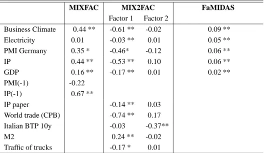
Table 1: Estimated factor loadings

MIXFAC MIX2FAC FaMIDAS Factor 1 Factor 2 Business Climate 0.44 ** -0.61 ** -0.02 0.09 ** Electricity 0.01 -0.03 ** 0.01 0.05 ** PMI Germany 0.35 * -0.46* -0.12 0.06 ** IP 0.44 ** -0.53 ** 0.10 0.06 ** GDP 0.16 ** -0.17 ** 0.01 0.02 ** PMI(-1) -0.22 IP(-1) 0.67 ** IP paper -0.14 ** 0.03 World trade (CPB) -0.74 ** 0.17 Italian BTP 10y -0.03 -0.37** M2 0.24 ** -0.02 Traffic of trucks -0.17 * 0.01 ** Means significant at 5%, * at 10%.

The sample period ranges from 1990M1 to 2009M4. Business Climate is provided by ISAE; Electricity is the monthly consumption of electricity provided by TERNA; PMI Germany is the Purchase Manager Index for Germany in manufacturing and services; IP paper is the Industrial production of paper and cardboard; World trade is the indica-tor of trade produced by the CPB- Netherlands Bureau for Economic Policy Analysis; Money supply includes currency and deposits; Motorway flow refers to trucks and it is provided by Autostrade

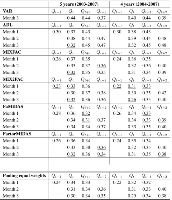
Table 2: Rolling forecasting experiment: RMSE. 5 years (2003-2007) 4 years (2004-2007) VAR 𝑄𝑡₋1 𝑄𝑡 𝑄𝑡+1 𝑄𝑡+2 𝑄𝑡₋1 𝑄𝑡 𝑄𝑡+1 𝑄𝑡+2 Month 3 0.44 0.44 0.37 0.40 0.44 0.39 ADL 𝑄𝑡−1 𝑄𝑡 𝑄𝑡+1 𝑄𝑡+2 𝑄𝑡−1 𝑄𝑡 𝑄𝑡+1 𝑄𝑡+2 Month 1 0.30 0.37 0.43 0.30 0.38 0.43 Month 2 0.38 0.44 0.47 0.39 0.44 0.48 Month 3 0.32 0.45 0.47 0.32 0.45 0.48 MIXFAC 𝑄𝑡−1 𝑄𝑡 𝑄𝑡+1 𝑄𝑡+2 𝑄𝑡−1 𝑄𝑡 𝑄𝑡+1 𝑄𝑡+2 Month 1 0.26 0.37 0.35 0.24 0.36 0.35 Month 2 0.33 0.37 0.36 0.32 0.36 0.40 Month 3 0.32 0.35 0.35 0.31 0.34 0.39 MIX2FAC 𝑄𝑡−1 𝑄𝑡 𝑄𝑡+1 𝑄𝑡+2 𝑄𝑡−1 𝑄𝑡 𝑄𝑡+1 𝑄𝑡+2 Month 1 0.23 0.33 0.36 0.22 0.31 0.33 Month 2 0.30 0.37 0.38 0.30 0.35 0.42 Month 3 0.32 0.36 0.36 0.26 0.35 0.40 FaMIDAS 𝑄𝑡−1 𝑄𝑡 𝑄𝑡+1 𝑄𝑡+2 𝑄𝑡−1 𝑄𝑡 𝑄𝑡+1 𝑄𝑡+2 Month 1 0.28 0.36 0.32 0.26 0.34 0.33 Month 2 0.34 0.31 0.37 0.34 0.33 0.39 Month 3 0.34 0.34 0.37 0.33 0.35 0.40 FactorMIDAS 𝑄𝑡₋1 𝑄𝑡 𝑄𝑡+1 𝑄𝑡+2 𝑄𝑡₋1 𝑄𝑡 𝑄𝑡+1 𝑄𝑡+2 Month 1 0.26 0.36 0.34 0.24 0.35 0.34 Month 2 0.33 0.38 0.36 0.32 0.35 0.40 Month 3 0.32 0.36 0.34 0.31 0.35 0.38

Pooling equal weights 𝑄𝑡−1 𝑄𝑡 𝑄𝑡+1 𝑄𝑡+2 𝑄𝑡−1 𝑄𝑡 𝑄𝑡+1 𝑄𝑡+2

Month 1 0.24 0.34 0.33 0.22 0.32 0.32

Month 2 0.31 0.34 0.36 0.31 0.33 0.40

Month 3 0.30 0.34 0.35 0.29 0.34 0.38

Note: Each entry represents the RMSE of the rolling forecast of GDP growth rates, aggregated to the quarterly frequency, by month of the quarter in which the prevision is made, horizon of prevision and window length. The best values among the models (except for the pooling) are underlined. The VAR is estimated on a balanced quarterly sample. The ADL is estimated as documented by Proietti (2006) by using the routines provided by the author.

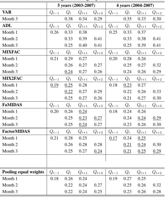
Table 3: Rolling forecasting experiment: MAPE. 5 years (2003-2007) 4 years (2004-2007) VAR 𝑄𝑡₋1 𝑄𝑡 𝑄𝑡+1 𝑄𝑡+2 𝑄𝑡₋1 𝑄𝑡 𝑄𝑡+1 𝑄𝑡+2 Month 3 0.38 0.34 0.29 0.35 0.33 0.30 ADL 𝑄𝑡−1 𝑄𝑡 𝑄𝑡+1 𝑄𝑡+2 𝑄𝑡−1 𝑄𝑡 𝑄𝑡+1 𝑄𝑡+2 Month 1 0.26 0.33 0.38 0.25 0.33 0.37 Month 2 0.33 0.39 0.41 0.33 0.38 0.41 Month 3 0.25 0.40 0.41 0.25 0.39 0.41 MIXFAC 𝑄𝑡−1 𝑄𝑡 𝑄𝑡+1 𝑄𝑡+2 𝑄𝑡−1 𝑄𝑡 𝑄𝑡+1 𝑄𝑡+2 Month 1 0.21 0.29 0.27 0.20 0.28 0.26 Month 2 0.26 0.27 0.27 0.25 0.27 0.32 Month 3 0.24 0.27 0.26 0.24 0.26 0.29 MIX2FAC 𝑄𝑡−1 𝑄𝑡 𝑄𝑡+1 𝑄𝑡+2 𝑄𝑡−1 𝑄𝑡 𝑄𝑡+1 𝑄𝑡+2 Month 1 0.19 0.25 0.28 0.18 0.23 0.27 Month 2 0.22 0.27 0.29 0.22 0.26 0.33 Month 3 0.25 0.27 0.26 0.21 0.27 0.30 FaMIDAS 𝑄𝑡−1 𝑄𝑡 𝑄𝑡+1 𝑄𝑡+2 𝑄𝑡−1 𝑄𝑡 𝑄𝑡+1 𝑄𝑡+2 Month 1 0.20 0.26 0.24 0.18 0.24 0.26 Month 2 0.25 0.23 0.27 0.24 0.24 0.29 Month 3 0.25 0.24 0.27 0.23 0.26 0.30 FactorMIDAS 𝑄𝑡₋1 𝑄𝑡 𝑄𝑡+1 𝑄𝑡+2 𝑄𝑡₋1 𝑄𝑡 𝑄𝑡+1 𝑄𝑡+2 Month 1 0.21 0.28 0.25 0.17 0.24 0.25 Month 2 0.26 0.28 0.28 0.21 0.24 0.30 Month 3 0.25 0.27 0.24 0.21 0.25 0.29

Pooling equal weights 𝑄𝑡−1 𝑄𝑡 𝑄𝑡+1 𝑄𝑡+2 𝑄𝑡−1 𝑄𝑡 𝑄𝑡+1 𝑄𝑡+2

Month 1 0.18 0.26 0.24 0.19 0.27 0.25

Month 2 0.22 0.24 0.27 0.25 0.26 0.32

Month 3 0.22 0.24 0.25 0.23 0.26 0.28

Note: Each entry represents the MAE of the rolling forecast of GDP growth rates, aggregated to the quarterly frequency, by month of the quarter in which the prevision is made, horizon of prevision and window length. The best values among the models (except for the pooling) are underlined. The VAR is estimated on a balanced quarterly sample. The ADL is estimated as documented by Proietti (2006) by using the routines provided by the author.

Table 4: Diebold-Mariano test by horizon of previsions and month in the quarter (Student-T).

QUADRATIC VALUES FaMIDAS versus Mixfac

1step 2step 3step Month 1 2.6 -0.8 -2.5 Month 2 0.7 -2.7 0.3 Month 3 1.7 -1.5 2.4 Overall 1.4 -1.6 -0.5

FaMIDAS versus Mix2fac 1step 2step 3step Month 1 3.6 3.4 -1.6 Month 2 4.6 -2.8 -1.6 Month 3 0.8 -1.8 0.8 Overall 2.0 -1.0 -0.8

FaMIDAS versus FactorMIDAS 1step 2step 3step Month 1 2.8 0.1 -1.7 Month 2 0.8 -2.3 0.4 Month 3 1.4 -1.9 3.8 Overall 1.4 -1.5 0.2

ABSOLUTE VALUES FaMIDAS versus Mixfac

1step 2step 3step Month 1 -1.8 -1.9 -2.7 Month 2 -0.3 -2.6 0.0 Month 3 0.4 -2.1 1.2 Overall -0.4 -2.1 -0.4

FaMIDAS versus Mix2fac 1step 2step 3step Month 1 3.6 3.4 -1.6 Month 2 4.6 -2.8 -1.6 Month 3 0.8 -1.8 0.8 Overall 2.0 -1.0 -0.8

FaMIDAS versus FactorMIDAS 1step 2step 3step Month 1 -2.2 -1.3 -1.4 Month 2 -0.4 -2.5 -0.2 Month 3 0.0 -2.5 2.2 Overall -0.7 -2.0 0.3 Note: Rolling forecast window: 2003-2007; Values adjusted by the Newey-West correction.

Figure 1: Monthly Indicators and Quarterly GDP- Italy 1990 1993 1996 1999 2002 2005 2008 60 80 100 Business climate 1990 1993 1996 1999 2002 2005 2008 17.5 20.0 22.5 25.0 _{Electricity Consumption} 1990 1993 1996 1999 2002 2005 2008 40 50

60 PMI Index Germany

1990 1993 1996 1999 2002 2005 2008 90 100 110 Industrial Production 1990 1993 1996 1999 2002 2005 2008 100 150 200 World trade 1990 1993 1996 1999 2002 2005 2008 275000 300000 325000 Quarterly GDP 1990 1993 1996 1999 2002 2005 2008 300000 350000 400000 Production of paper 1990 1993 1996 1999 2002 2005 2008 6000 7000 8000 9000 10000 11000 M2 1990 1993 1996 1999 2002 2005 2008 0.05 0.10 0.15 0.20 Italian BTP 10 y (deflated) 1990 1993 1996 1999 2002 2005 2008 100 120

Traffic of tracks (Index 2000=100)

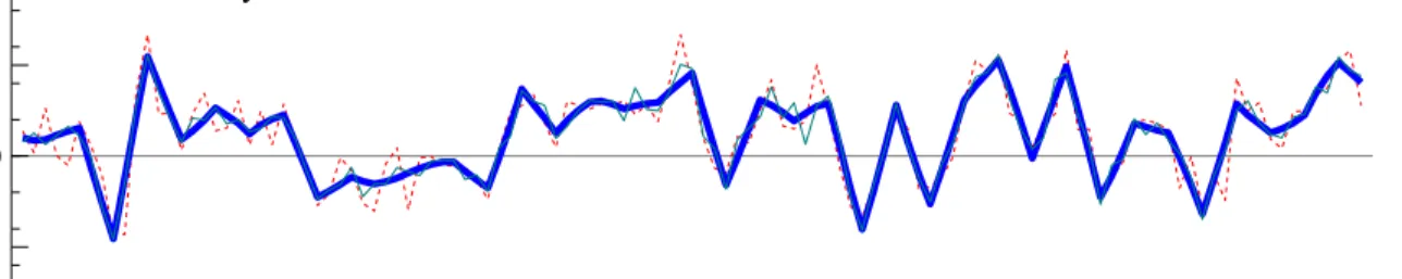
2

Figure 2: Estimated Monthly GDP and common factors . 2000 2001 2002 2003 2004 2005 2006 2007 2008 2009 −0.010 −0.005 0.000 0.005

GDP Monthly Growth Rates

MIXFAC MIX2FACT FaMIDAS 1990 1992 1994 1996 1998 2000 2002 2004 2006 2008 0 25 50 Common Factor MIXFAC MIX2FACT−Factor 1 FaMIDAS MIX2FACT−Factor 2 1990 1991 1992 1993 1994 1995 1996 1997 1998 1999 2000 −0.010 −0.005 0.000 0.005 0.010

Figure 3: Forecasts and fan charts 2006 2007 2008 106000 108000 110000 FaMIDAS 2006 2007 2008 MIX2FAC 2006 2007 2008 MIXFAC 2 8

Figure 4: Spectral Density of the Monthly GDP. 0.0 0.2 0.4 0.6 0.8 1.0 0.0 0.2 0.4 0.6 0.8 1.0 0.0 0.2 0.4 0.6 0.8 1.0 0.1 0.2 0.3 0.4 0.5 0.6 0.7 0.8 0.9 1.0 Spectral density MIXFAC MIX2FAC FaMIDAS

Note: The horizontal axis represents frequencies from 0 to𝜋, while on the vertical axis the estimated spectral density of the monthly GDP in growth rates.

(*) Requests for copies should be sent to:

Banca d’Italia – Servizio Studi di struttura economica e finanziaria – Divisione Biblioteca e Archivio storico – Via

RECENTLY PUBLISHED “TEMI” (*)

N. 762 – A public guarantee of a minimum return to defined contribution pension scheme

members, by Giuseppe Grande and Ignazio Visco (June 2010).

N. 763 – Debt restructuring and the role of lending technologies, by Giacinto Micucci and Paola Rossi (June 2010).

N. 764 – Disentangling demand and supply in credit developments: a survey-based analysis

for Italy, by Paolo Del Giovane, Ginette Eramo and Andrea Nobili (June 2010).

N. 765 – Information uncertainty and the reaction of stock prices to news, by Paolo Angelini and Giovanni Guazzarotti (July 2010).

N. 766 – With a little help from abroad: the effect of low-skilled immigration on the female

labor supply, by Guglielmo Barone and Sauro Mocetti (July 2010).

N. 767 – Real time forecasts of inflation: the role of financial variables, by Libero Monteforte and Gianluca Moretti (July 2010).

N. 768 – The effect of age on portfolio choices: evidence from an Italian pension fund, by Giuseppe G. L. Cappelletti, Giovanni Guazzarotti and Pietro Tommasino (July 2010). N. 769 – Does investing abroad reduce domestic activity? Evidence from Italian

manufacturing firms, by Raffaello Bronzini (July 2010).

N. 770 – The EAGLE. A model for policy analysis of macroeconomics interdependence in the

euro area, by Sandra Gomes, Pascal Jacquinot and Massimiliano Pisani (July 2010).

N. 771 – Modelling Italian potential output and the output gap, by Antonio Bassanetti, Michele Caivano and Alberto Locarno (September 2010).

N. 772 – Relationship lending in a financial turmoil, by Stefania De Mitri, Giorgio Gobbi and Enrico Sette (September 2010).

N. 773 – Firm entry, competitive pressures and the US inflation dynamics, by Martina Cecioni (September 2010).

N. 774 – Credit ratings in structured finance and the role of systemic risk, by Roberto Violi (September 2010).

N. 775 – Entrepreneurship and market size. The case of young college graduates in Italy, by Sabrina Di Addario and Daniela Vuri (September 2010).

N. 776 – Measuring the price elasticity of import demand in the destination markets of

Italian exports, by Alberto Felettigh and Stefano Federico (October 2010).

N. 777 – Income reporting behaviour in sample surveys, by Andrea Neri and Roberta Zizza (October 2010).

N. 778 – The rise of risk-based pricing of mortgage interest rates in Italy, by Silvia Magri and Raffaella Pico (October 2010).

N. 779 – On the interaction between market and credit risk: a factor-augmented vector

autoregressive (FAVAR) approach, by Roberta Fiori and Simonetta Iannotti

(October 2010).

N. 780 – Under/over-valuation of the stock market and cyclically adjusted earnings, by Marco Taboga (December 2010).

N. 781 – Changing institutions in the European market: the impact on mark-ups and

rents allocation, by Antonio Bassanetti, Roberto Torrini and Francesco Zollino

(December 2010).

N. 782 – Central bank’s macroeconomic projections and learning, by Giuseppe Ferrero and Alessandro Secchi (December 2010).

N. 783 – (Non)persistent effects of fertility on female labour supply, by Concetta Rondinelli and Roberta Zizza (December 2010).

"TEMI" LATER PUBLISHED ELSEWHERE

2008

P. ANGELINI, Liquidity and announcement effects in the euro area, Giornale degli Economisti e Annali di

Economia, v. 67, 1, pp. 1-20, TD No. 451 (October 2002).

P.ANGELINI,P.DEL GIOVANE,S.SIVIERO and D.TERLIZZESE,Monetary policy in a monetary union: What

role for regional information?, International Journal of Central Banking, v. 4, 3, pp. 1-28, TD No. 457 (December2002).

F. SCHIVARDI and R. TORRINI, Identifying the effects of firing restrictions through size-contingent

Differences in regulation,Labour Economics, v. 15, 3, pp. 482-511, TDNo.504(June2004).

L. GUISO and M. PAIELLA,, Risk aversion, wealth and background risk, Journal of the European Economic Association, v. 6, 6, pp. 1109-1150, TD No. 483 (September2003).

C.BIANCOTTI,G.D'ALESSIO andA. NERI, Measurement errors in the Bank of Italy’s survey of household

income and wealth, Review of Income and Wealth, v. 54, 3, pp. 466-493, TD No. 520 (October 2004).

S. MOMIGLIANO, J. HENRY and P. HERNÁNDEZ DE COS, The impact of government budget on prices:

Evidence from macroeconometric models, Journal of Policy Modelling, v. 30, 1, pp. 123-143 TD No. 523 (October 2004).

L.GAMBACORTA,How do banks set interest rates?, European Economic Review, v. 52, 5, pp. 792-819,

TD No. 542 (February2005).

P. ANGELINI and A. GENERALE, On the evolution of firm size distributions, American Economic Review,

v. 98, 1, pp. 426-438, TD No. 549 (June 2005).

R. FELICI and M. PAGNINI, Distance, bank heterogeneity and entry in local banking markets, The Journal

of Industrial Economics, v. 56, 3, pp. 500-534, No. 557 (June 2005).

S. DI ADDARIO andE.PATACCHINI, Wages and the city. Evidence from Italy, Labour Economics, v.15, 5,

pp. 1040-1061, TD No. 570 (January 2006).

S.SCALIA,Is foreign exchange intervention effective?,Journal of International Money and Finance, v. 27, 4,

pp. 529-546,TD No. 579 (February2006).

M.PERICOLI and M.TABOGA, Canonical term-structure models with observable factors and the dynamics

of bond risk premia, Journal of Money, Credit and Banking, v. 40, 7, pp. 1471-88,TD No. 580 (February 2006).

E. VIVIANO, Entry regulations and labour market outcomes. Evidence from the Italian retail trade sector,

Labour Economics, v. 15, 6, pp. 1200-1222, TD No. 594 (May 2006).

S.FEDERICO andG.A.MINERVA,Outward FDI and local employment growth in Italy, Review of World

Economics, Journal of Money, Credit and Banking, v. 144, 2, pp. 295-324,TD No.613(February 2007).

F.BUSETTI and A.HARVEY, Testing for trend, Econometric Theory, v. 24, 1, pp. 72-87, TD No. 614

(February 2007).

V. CESTARI,P.DEL GIOVANE andC.ROSSI-ARNAUD, Memory for prices and the Euro cash changeover: an

analysis for cinema prices in Italy, In P. Del Giovane e R. Sabbatini (eds.), The Euro Inflation and Consumers’ Perceptions. Lessons from Italy, Berlin-Heidelberg, Springer, TD No. 619 (February 2007).

B. H. HALL,F.LOTTI and J. MAIRESSE, Employment, innovation and productivity: evidence from Italian manufacturing microdata, Industrial and Corporate Change, v. 17, 4, pp. 813-839, TD No. 622 (April 2007).

J. SOUSA and A. ZAGHINI, Monetary policy shocks in the Euro Area and global liquidity spillovers,

International Journal of Finance and Economics, v.13, 3, pp. 205-218, TD No. 629 (June 2007).

M. DEL GATTO,GIANMARCO I. P. OTTAVIANO and M. PAGNINI, Openness to trade and industry cost

dispersion: Evidence from a panel of Italian firms, Journal of Regional Science, v. 48, 1, pp. 97-129, TD No. 635 (June 2007).

P. DEL GIOVANE,S. FABIANI and R. SABBATINI, What’s behind “inflation perceptions”? A survey-based

analysis of Italian consumers, in P. Del Giovane e R. Sabbatini (eds.), The Euro Inflation and Consumers’ Perceptions. Lessons from Italy, Berlin-Heidelberg, Springer, TD No. 655 (January 2008).

B.BORTOLOTTI,andP.PINOTTI, Delayed privatization, Public Choice, v. 136, 3-4, pp. 331-351, TD No. 663 (April 2008).

R. BONCI andF.COLUMBA, Monetary policy effects: New evidence from the Italian flow of funds, Applied

Economics , v. 40, 21, pp. 2803-2818, TD No. 678 (June 2008).

M.CUCCULELLI,andG.MICUCCI, Family Succession and firm performance: evidence from Italian family

firms, Journal of Corporate Finance, v. 14, 1, pp. 17-31, TD No. 680 (June 2008).

A.SILVESTRINI andD.VEREDAS, Temporal aggregation of univariate and multivariate time series models:

a survey, Journal of Economic Surveys, v. 22, 3, pp. 458-497, TD No. 685 (August 2008).

2009

F.PANETTA,F.SCHIVARDI andM.SHUM, Do mergers improve information? Evidence from the loan market,

Journal of Money, Credit, and Banking, v. 41, 4, pp. 673-709, TD No. 521 (October 2004).

M. BUGAMELLI and F. PATERNÒ, Do workers’ remittances reduce the probability of current account

reversals?, World Development, v. 37, 12, pp. 1821-1838, TD No. 573 (January 2006).

P. PAGANO andM.PISANI, Risk-adjusted forecasts of oil prices, The B.E. Journal of Macroeconomics, v.

9, 1, Article 24, TD No. 585 (March 2006).

M. PERICOLI and M. SBRACIA, The CAPM and the risk appetite index: theoretical differences, empirical

similarities, and implementation problems, International Finance, v. 12, 2, pp. 123-150, TD No. 586 (March 2006).

U. ALBERTAZZI and L. GAMBACORTA, Bank profitability and the business cycle, Journal of Financial

Stability, v. 5, 4, pp. 393-409, TD No. 601 (September 2006).

S.MAGRI,The financing of small innovative firms: the Italian case, Economics of Innovation and New Technology, v. 18, 2, pp. 181-204, TD No. 640 (September 2007).

V. DI GIACINTO and G. MICUCCI, The producer service sector in Italy: long-term growth and its local

determinants, Spatial Economic Analysis, Vol. 4, No. 4, pp. 391-425, TD No. 643 (September 2007).

F.LORENZO,L.MONTEFORTE andL.SESSA, The general equilibrium effects of fiscal policy: estimates for the

euro area, Journal of Public Economics, v. 93, 3-4, pp. 559-585, TD No. 652 (November 2007).

R. GOLINELLI andS.MOMIGLIANO, The Cyclical Reaction of Fiscal Policies in the Euro Area. A Critical

Survey of Empirical Research, Fiscal Studies, v. 30, 1, pp. 39-72, TD No. 654 (January 2008).

P.DEL GIOVANE,S.FABIANI andR.SABBATINI, What’s behind “Inflation Perceptions”? A survey-based

analysis of Italian consumers, Giornale degli Economisti e Annali di Economia, v. 68, 1, pp. 25-52, TD No. 655 (January2008).

F.MACCHERONI,M.MARINACCI,A.RUSTICHINI andM.TABOGA, Portfolio selection with monotone

mean-variance preferences, Mathematical Finance, v. 19, 3, pp. 487-521, TD No. 664 (April 2008).

M. AFFINITO and M. PIAZZA, What are borders made of? An analysis of barriers to European banking

integration, in P. Alessandrini, M. Fratianni and A. Zazzaro (eds.): The Changing Geography of Banking and Finance, Dordrecht Heidelberg London New York, Springer, TD No. 666 (April 2008).

A. BRANDOLINI, On applying synthetic indices of multidimensional well-being: health and income

inequalities in France, Germany, Italy, and the United Kingdom, in R. Gotoh and P. Dumouchel (eds.), Against Injustice. The New Economics of Amartya Sen, Cambridge, Cambridge University Press, TD No. 668 (April 2008).

G. FERRERO andA.NOBILI, Futures contract rates as monetary policy forecasts, International Journal of

Central Banking, v. 5, 2, pp. 109-145, TD No. 681 (June 2008).

P. CASADIO,M.LO CONTE andA.NERI, Balancing work and family in Italy: the new mothers’ employment

decisions around childbearing, in T. Addabbo and G. Solinas (eds.), Non-Standard Employment and Qualità of Work, Physica-Verlag. A Sprinter Company, TD No. 684 (August 2008).

L.ARCIERO,C.BIANCOTTI,L.D'AURIZIO andC.IMPENNA, Exploring agent-based methods for the analysis

of payment systems: A crisis model for StarLogo TNG, Journal of Artificial Societies and Social Simulation, v. 12, 1, TD No. 686 (August 2008).

A. CALZA and A. ZAGHINI, Nonlinearities in the dynamics of the euro area demand for M1,

Macroeconomic Dynamics, v. 13, 1, pp. 1-19, TD No. 690 (September 2008).

L. FRANCESCO andA.SECCHI, Technological change and the households’ demand for currency, Journal of

Monetary Economics, v. 56, 2, pp. 222-230, TD No. 697 (December 2008).

S. COLAROSSI andA.ZAGHINI, Gradualism, transparency and the improved operational framework: a look at overnight volatility transmission, International Finance, v. 12, 2, pp. 151-170, TD No. 710 (May 2009).

M. BUGAMELLI,F.SCHIVARDI andR.ZIZZA, The euro and firm restructuring, in A. Alesina e F. Giavazzi

(eds): Europe and the Euro, Chicago, University of Chicago Press, TD No. 716 (June 2009).

B.HALL,F.LOTTI andJ.MAIRESSE, Innovation and productivity in SMEs: empirical evidence for Italy,

Small Business Economics, v. 33, 1, pp. 13-33, TD No. 718 (June 2009).

2010

A. PRATI and M. SBRACIA, Uncertainty and currency crises: evidence from survey data, Journal of Monetary Economics, v, 57, 6, pp. 668-681, TD No. 446 (July 2002).

S.MAGRI, Debt maturity choice of nonpublic Italian firms , Journal of Money, Credit, and Banking, v.42, 2-3, pp. 443-463, TD No. 574 (January 2006).

R.BRONZINI andP.PISELLI,Determinants of long-run regional productivity with geographical spillovers:

the role of R&D, human capital and public infrastructure, Regional Science and Urban Economics, v. 39, 2, pp.187-199, TDNo.597(September 2006).

E.IOSSA andG. PALUMBO,Over-optimism and lender liability in the consumer credit market, Oxford

Economic Papers, v. 62, 2, pp. 374-394, TDNo.598(September 2006).

S. NERI andA.NOBILI, The transmission of US monetary policy to the euro area, International Finance, v.

13, 1, pp. 55-78, TD No. 606 (December 2006).

F.ALTISSIMO,R.CRISTADORO,M.FORNI,M.LIPPI andG.VERONESE, New Eurocoin: Tracking Economic

Growth in Real Time, Review of Economics and Statistics, v. 92, 4, pp. 1024-1034, TD No. 631 (June 2007).

A.CIARLONE,P.PISELLI andG.TREBESCHI,Emerging Markets' Spreads and Global Financial Conditions,

Journal of International Financial Markets, Institutions & Money, v. 19, 2, pp. 222-239, TD No. 637 (June 2007).

U.ALBERTAZZI and L.GAMBACORTA, Bank profitability and taxation, Journal of Banking and Finance, v.

34, 11, pp. 2801-2810, TD No. 649 (November 2007).

M. IACOVIELLO and S. NERI, Housing market spillovers: evidence from an estimated DSGE model,

American Economic Journal: Macroeconomics, v. 2, 2, pp. 125-164,TD No. 659 (January 2008).

F.BALASSONE,F.MAURA andS.ZOTTERI,Cyclical asymmetry in fiscal variables in the EU, Empirica, TD

No. 671, v. 37, 4, pp. 381-402 (June 2008).

F.D'AMURI,O.GIANMARCO I.P. and P.GIOVANNI, The labor market impact of immigration on the western

german labor market in the 1990s, European Economic Review, v. 54, 4, pp. 550-570, TD No. 687 (August 2008).

A.ACCETTURO, Agglomeration and growth: the effects of commuting costs, Papers in Regional Science, v.

89, 1, pp. 173-190, TD No. 688 (September 2008).

S.NOBILI andG.PALAZZO, Explaining and forecasting bond risk premiums, Financial Analysts Journal, v.

66, 4, pp. 67-82, TD No. 689 (September 2008).

A. B. ATKINSON and A. BRANDOLINI, On analysing the world distribution of income, World Bank

Economic Review , v. 24, 1 , pp. 1-37, TD No. 701 (January 2009).

R.CAPPARIELLO and R.ZIZZA, Dropping the Books and Working Off the Books, Labour, v. 24, 2, pp.

139-162 ,TD No. 702 (January 2009).

C.NICOLETTI andC.RONDINELLI, The (mis)specification of discrete duration models with unobserved

heterogeneity: a Monte Carlo study, Journal of Econometrics, v. 159, 1, pp. 1-13, TD No. 705 (March 2009).

V.DI GIACINTO, G. MICUCCI andP. MONTANARO, Dynamic macroeconomic effects of public capital:

evidence from regional Italian data, Giornale degli economisti e annali di economia, v. 69, 1, pp. 29-66,TD No. 733 (November 2009).

F.COLUMBA,L.GAMBACORTA and P.E.MISTRULLI, Mutual Guarantee institutions and small business

finance, Journal of Financial Stability, v. 6, 1, pp. 45-54, TD No. 735 (November 2009).

A.GERALI,S.NERI,L.SESSA andF.M.SIGNORETTI, Credit and banking in a DSGE model of the Euro