Mobile Edge Cloud Network Design Optimization
Alberto Ceselli, Marco Premoli, and Stefano Secci,
Senior Member, IEEE
Abstract—Major interest is currently given to the integration of clusters of virtualization servers, also referred to as ‘cloudlets’ or ‘edge clouds’, into the access network to allow higher perfor-mance and reliability in the access to mobile edge computing services. We tackle the edge cloud network design problem for mobile access networks. The model is such that virtual machines are associated with mobile users and are allocated to cloudlets. Designing an edge cloud network implies first determining where to install cloudlet facilities among the available sites, then assigning sets of access points such as base-stations to cloudlets, while supporting virtual machine orchestration and taking into account partial user mobility information, as well as the satisfaction of service-level agreements. We present link-path formulations supported by heuristics to compute solutions in reasonable time. We qualify the advantage in considering mobility for both users and virtual machines as up to 20% less users not satisfied in their SLA with little increase of opened facilities. We compare two VM mobility modes, bulk and live migration, as a function of mobile cloud service requirements, determining that a high preference should be given to live migration, while bulk migrations seems to be a feasible alternative on delay-stringent tiny-disk services such as augmented reality support, and only with further relaxation on network constraints.
Index Terms—Mobile Edge Computing, Cloud networking.
I. INTRODUCTION
M
OBILE devices are ubiquitous in people’s everyday life, with a remarkable growth of mobile data traffic over recent years [2]. As mobile applications become increas-ingly resource-hungry, the gap between required resources and those available in mobile devices widens. To bridge this gap, cloud computing can be used to expand mobile devices resources. To deal with high latency of distant cloud center, the concept of cloudlet was introduced in [3] where it is defined as a trusted, resource-rich computer or cluster of computers well-connected to the Internet and available for use by nearby mobile devices. A cloudlet represents a container for virtual machines (VMs): connected users are associated with VMs supporting low-latency application offloading use-cases.Cloudlet concept is expected to be supported by 3-tier hierarchical network provisioning as presented in [4] and [5]. In this hierarchy the cloudlet is the primal resource for the augmentation of the mobile device capabilities, while a remote cloud is used as last available resource, or for delay-tolerant resource-intensive applications. Telecommunication vendors and providers show an increasing interest in such deployments, also referred to as ‘mobile edge computing’ (MEC) solutions in industrial fora and standardization bodies (e.g. [6], [7]).
A. Ceselli and M. Premoli are with the Department of Computer Science, Universit`a degli Studi di Milano, Italy. e-mail: first-name.last-name@unimi.it. S. Secci is with the UPMC Univ Paris 06, UMR 7606, LIP6, F-75005, Paris, France. e-mail: stefano.secci@upmc.fr.
A preliminary version of the content of this paper is presented in [1].
Within this framework, in this paper we focus on the poten-tial medium-term planning of an edge cloud network in mobile access networks, which is, to the best of our knowledge, an untreated problem in the literature. This consists in the placement of all virtualization infrastructure resources, from the access points to the cloudlets, together with the assignment of users to cloudlets. We investigate two design cases: (i) with a network in a static state and (ii) with the network state variations in terms of load and service level, caused by user mobility. In this latter case we include orchestration of virtual resources, in particular VM orchestration across cloudlets, in order to re-balance the system. Our contribution is as follows:
• We provide a link-path mixed integer linear programming
formulation including a polynomial number of variables to represent location and design decisions, and an expo-nential number of them to encode routing ones.
• Since adaptations of heuristics from the literature are un-able to produce accurate results, we exploit mathematical programming techniques, combining column generation [8], iterative rounding, local search, very large scale neighborhood and problem reduction to achieve high quality solutions in reasonable time.
• We bring novel and original insights on the planning of cloudlets for mobile access networks. By performing extensive simulations on real 4G cellular network data-sets from the ˆIle-de-France Orange network, we show the trade-off that can be achieved by means of the two design cases and the impact of user mobility on the cloudlet network: as few as 13 to 26 cloudlets can be planned for 180 thousands of users while requiring tight delay guarantees. We show that there is a sensible gain in the number of users with respected SLA, up to 20%, by including user and VM mobility in the network planning. We do also qualify the eligibility of two different VM mobility strategies, namely VM bulk and live migrations, for two reference mobile cloud services differing in the level of required latency and memory characteristics: augmented-reality and remote desktop.
• We report empirical distributions of the dataset features
in order to allow the reproducibility of our results. In [1] we provide a preliminary modeling of the mobile edge cloud network design problem. In this paper we re-fine the model and we provide a new heuristic including a dynamic decomposition logic. Furthermore, we present a more detailed set of results, carrying out a substantially deeper analysis of policies and practices. The paper is orga-nized as follows. Sect. II presents the background. Sect. III presents cloudlet network models and related mathematical formulations. Sect. V presents the dataset. Sect. VI reports experimental results and Sect. VII contains brief conclusions.
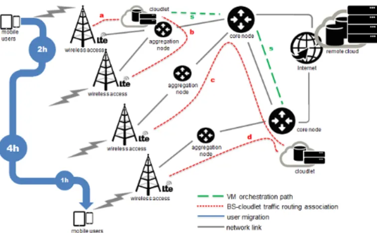
Fig. 1: Example of a simplified mobile edge cloud network.
II. BACKGROUND
Benefits of cloudlet usage on users’ QoE are presented in [9]–[11] where authors compare performances of different types of applications on different layers of the 3-tier hier-archy. In [9] authors show that application placement can significantly impact performance and user experience moving applications closer to the users. Authors of [10] question, by quantitative experimental results, benefits from consolidating computing resources in large data centers when strict latency constraints are required. Considering multi-hop WiFi net-works, in [11] authors show that the cloudlet-based approach always outperforms the cloud-based one when no more than two wireless hops are used to transfer data, and that up to a maximum of four hops the cloudlet-based approach is the best one for most of the instances. There is no binding dependence on the nature of the wireless link: even if the seminal idea was to use cloudlet via WiFi, the virtualization architecture is independent of it. A further survey on researches on cloudlet based mobile computing is available in [12].
Hardware technologies for the implementation of cloudlets already exist, thanks to fabrics called ‘micro data centers’ or ‘modular data center’ [13]–[15]. A standardization effort is sustained by the European Telecommunications Standard-ization Institute (ETSI) that in [6], [7] provides technical re-quirements for a deployment of a mobile edge cloud network, together with use-cases examples such as augmented reality, Internet-of-Things (IoT) and data caching among others. In this work we primarily address application VMs rather than virtual network functions.
A. VM mobility technologies
In Section III.D we deal with the dynamic state of the network, whose variations generate imbalances and users’ SLA violations. To re-balance the system, we include VM mobility from cloudlet to cloudlet in the model, considering three VM mobility technologies at the state of the art:
• VM bulk migration[16]: consists in migrating the whole
VM stack including disk and memory, stopping the VM for a long period to transfer it.
• VM live migration [17]–[19]: stops the VM only for a
small amount of time required to transfer the most
re-cently used memory, not requiring an entire one-shot disk transfer, but a permanent disk storage synchronization among source and destination locations.
• VM replication [20]: consists in a permanent
synchro-nization of both disk storage and memory among source and destination locations, not requiring the point transfer neither of the disk nor of the most recently used memory. We assume VM orchestrations to be performed in a Cloud Stack platform in a centralized way. Given that the main pur-pose of our model is the medium-term planning of the mobile edge cloud network, the inclusion of VM orchestration has the aim of providing a correct dimensioning of the network. Hence an actual implementation of such a system is out of scope of this work, but examples are already present (e.g. in OpenStack platform [21], [22]).
B. Mobile Edge Cloud Network Topology
Accordingly to the ETSI [6], [7], the distribution of comput-ing resources into mobile access network should be carefully designed to take into account infrastructure properties. Mo-bile access networks could be any form of wireless access network disposing of a backhauling wireline infrastructure through which cloudlets can be interconnected. Following the guidelines in [23]–[26], a broadband access and back-hauling network, such as a cellular network, can be modeled as a two-level hierarchical network: access points on the field are connected to aggregation nodes, which are then connected to core nodes, as depicted in Fig. 1 (for simplicity, we refer in the following to access points as APs). The APs could be WiFi only, cellular only, or a mix of these common mobile access technologies. Cloudlets can reasonably be placed at either field, aggregation or core level, with connections between an AP and its cloudlet potentially crossing twice each level.
Various physical interconnection network topologies be-tween APs, aggregation nodes and core nodes are commonly adopted: tree, ring or mesh topologies, as well as intermediate hybrid topologies. Moreover, with the emergence of 4G, there is a trend to further mesh back-hauling nodes. A variety of net-work protocol architectures are typically adopted, from circuit-switched networks to carrier-grade packet-circuit-switched networks. The common denominator of such architectures is the ability to create a virtual topology of links directly interconnecting pairs of nodes at a same level with a guaranteed tunnel capacity. Nowadays, with the convergence towards packet-switching carrier-grade solutions at the expense of legacy circuit-switched approaches, bit-rates for pseudo-cables links is set to giga-Ethernet granularities (typically 1 or 10 Gbps).
In this framework, we believe it is appropriate to model the mobile edge cloud network as a superposition of stars of virtual links for the interconnection of aggregation nodes to APs and for the interconnection of core nodes to ag-gregation nodes, even if nodes can have no physical direct connection. Under the same virtual link provisioning trend, core nodes can be considered as interconnected to each other by a full mesh topology of virtual links, as depicted in Fig. 1. As far as we know, partitioning of traffic from one AP to multiple aggregation nodes, and from one aggregation
node to multiple core nodes is not the dominating current practice in backhauling networks; still, such features would not change significantly the nature of our modeling and heuristic described in the next two sections. It is worth noting that the decisions of associating APs to aggregation nodes and placing aggregation nodes can be fully compatible with the current trend of dynamically reprogramming the cellular back-hauling network [27]. Likewise, another customization could correspond to the routing re-optimization for a given cloudlet placement. Moreover, those decisions can also realistically embed association and placement functions in cloud-based Evolved Packet Core architectures [28].
III. MOBILEEDGECLOUDNETWORKMODEL
In the following, we give a formal definition of the cloudlet design dimensioning problem, and we propose two variants:
• Static planning (SP in the remainder): network status is
considered static in time; neither user mobility nor virtual machine mobility are taken into account when planning cloudlet placement, and associations of APs to cloudlets.
• Dynamic planning (DP in the remainder): variations in
the network load during the planning time horizon are taken into account together with user mobility. Adaptive VM mobility is included in a generalized way to consider three different technologies: VM bulk migrations, VM live migrations and VM replications.
A. Problem statement
Our models finds simultaneously: (i) an optimal network design, including cloudlet placement and assignment of APs to cloudlets, and (ii) an optimal routing of the traffic from and to the cloudlets. Its main aim is to provide strategic insights into optimal design policies rather than an operational planning.
From a practical perspective, placing a cloudlet at a location could mean turning on already installed servers, and not only physically installing new machines. Similarly, changing AP to cloudlet assignments would in practice correspond to a re-routing of virtual links over the transport network in-frastructure, and not physically changing the interconnection. We consider a solution to be feasible if users’ service level agreement is respected; optimal feasible solutions minimize a linear combination of overall installation costs.
Our problem turns out to be hard from both a theoretical and computational point of view. Theoretically, it is strongly NP-Hard, generalizing the traditional uncapacitated facility lo-cation problem and its capacitated and single-source variants. Computationally, it is on the cutting edge of those currently under investigation in the facility location literature [29]: state-of-the-art methods are successful when up to two facility levels are considered, but in our models routing optimization, latency bounds and a third location level must be included.
In the following, we introduce the basic models dealing with network design (in III.B); then we add routing aspects (in III.C), thereby completing them for the SP variant. Finally, we discuss how this modeling extends to the DP variant1.
1Complete notation tables for our models and heuristic are included in Appendix Tables A.I, A.II and A.III in Supplementary Materials.
B. Network design
Input (problem data). We assume that a set of suitable locations has been identified for hosting network facilities. Formally, letB be the set of AP locations. LetI,J andKbe the set of sites where aggregation, core nodes and cloudlet can be installed, resp.. Let alsoE⊆(B×I)∪(I×J)∪(J×J)
be the set of feasible links between nodes. Let li,mj,ck be the fixed cost for activating an aggregation node in i ∈I, a core node inj∈J and a cloudlet facility in k∈K, resp..
Output (decision variables).We introduce two sets of vari-ables. The first set corresponds to location binary variables: xi take value 1 if an aggregation node is set in i ∈ I; yj take value 1 if a core node is set in j ∈J; zk take value 1 if a cloudlet is set in k∈K. The second set corresponds to network topology binary variables:ts,i take value 1if anAP link is established between an APsand an aggregation node i;wi,jandwj,i simultaneously take value1if anaggregation link is established between an aggregation nodei and a core nodej;om,ntake value1if acorelink is established between two core nodes m andn. In order to model already existing or forbidden links, the corresponding variables can be fixed to value1 and0, resp..
Objective function Since our main purpose is the MEC network design, the model goal (1) is to minimize installation costs of all network facilities. We do not include the links installation costs as we do not take into consideration the cellular infrastructure dimensioning.
minX i∈I lixi+ X j∈J mjyj+ X k∈K ckzk (1)
Constraints. A complete MECnetwork topologyresults as a by-product of our model, in terms of arrangement of links. As specified in Section II.B we model this network as a superposition of stars: this has to be intended as atopological rule, which constrains the resulting arrangement of links. Each AP is connected to a single aggregation node, and each aggregation node to a single core node (as depicted in Fig. 1), while a full mesh is built among cores. The following set of constraints enforce our topological rules to be respected: each link (i, j) can be used only for one purpose (i.e. AP, aggregation or core) - (2); aggregation links must be symmetric - (3); core nodes and cloudlet nodes are also aggregation nodes - (4) and (5); if (i, j)is an AP link then j is an aggregation node - (9), while if(i, j)is an aggregation link, then i is an aggregation node - (10); if (i, j) is an aggregation link, then either i or j is a core node - (11) - and similarly if(i, j) is a core link, both i and j are core nodes - (12), conversely if both i and j are core nodes, (i, j) is a core link - (13), moreover no loops are considered at core links - (8); each AP is connected to either itself when chosen as aggregation, or a different node otherwise - (6) and (14); each aggregation node has an adjacent aggregation link, thereby connecting to a core node - (15), which can be the node itself - (7), at most one aggregation link can be connected to non-core nodes (yi= 0), while an arbitrary number can be connected to core ones (yi= 1) - (16).
ti,j+wi,j+oi,j≤1 ∀(i, j)∈E|i6=j (2) wi,j=wj,i ∀(i, j)∈E (3) xi≥yi ∀i∈N (4) xi≥zi ∀i∈N (5) ti,i=xi ∀i∈N (6) wj,j=yj ∀j∈N (7) oi,i= 0 ∀i∈N (8) ti,j≤xj ∀(i, j)∈E (9) wi,j≤xi ∀(i, j)∈E (10) wi,j≤yi+yj ∀(i, j)∈E|i6=j (11) 2·oi,j≤yi+yj ∀(i, j)∈E|i6=j (12) yi+yj−1≤oi,j ∀(i, j)∈E|i6=j (13) X i∈N |j6=i∧(i,j)∈E ti,j= 1−xj ∀i∈N (14) X j∈N:(i,j)∈E wi,j≥xi ∀i∈N (15) X j∈N |(i,j)∈E∧i6=j wi,j≤(1−yi) +|I| ·yi ∀i∈N (16) C. Static Planning
Input (problem data). Each AP s ∈ B can connect to a cloudlet located in k∈K by a set of paths S¯sk (see pathsa, b,canddin Fig. 1). Pathp∈S¯sk can traverse multiple sites and with j∈pwe denote that sitej is traversed by pathp.
For each AP s∈B, letδu
s andδbs be the number of users connected to sand their overall bandwidth consumption. We assume that servicing each user requires the activation of one VM, and therefore δus represents also the number of VMs needed for AP s. It is worth noting that considering multiple VMs per user (i.e., a generic Infrastructure as a Service) is straightforward and can be easily defined; conversely, sharing a VM by multiple users is not straightforward (and may not be the most common edge computing service deployment); these adaptations are out of scope and left to future work.
Let C be the number of VMs that each cloudlet can host. Let di,j and ui,j be the latency (latency or length are used interchangeably hereafter) and bandwidth capacity of each link
(i, j) ∈ E. Let U ∈ [0,1] be the parameter representing the maximum link utilization (percentage) in the network; indeed, as a common practice in IP traffic engineering with non deterministic loads, links need to have a level of over-provisioning so that they are robust against traffic fluctuations (due to failures, traffic peaks, etc) and hence the risk of congestion, which is particularly important for real-time and interactive services as those considered by MEC [6], [7].
Finally, we consider static and identical SLAs for all users, defined as the maximum allowed latency a user may experience, assuming it to be represented by three types of constraints: (i) maximum sum of link length in a path D; (ii)¯ maximum number of hops in a path H¯ that according to [11] affects the effectiveness of cloudlets; (iii) maximum distance allowed between nodes in the network to establish a linkd. In¯
Section VI we provide a parametric analysis on these bounds, showing their influence on network planning decisions.2 Output (decision variables). To model routing decision we introduce an additional set of binary variables:rs,k
p take value
1 if users in APs∈B are served by cloudlet ink∈K, and the corresponding traffic is routed along pathp∈S¯sk.
Constraints.Feasible paths are those that satisfy SLA latency requirements defined previously. In order to enforce that only feasible paths are considered, we replace each set S¯sk with the following set:
Ssk={p∈S¯sk : X (i,j)∈p d(i,j)≤D¯∧ |p| ≤H¯ ∧ d(i,j)≤d¯∀(i, j)∈p} (17)
where by|p| we denote the number of links forming pathp. Constraints (18)-(20) impose that each path from APs∈B to cloudletk∈K, traversing either an aggregation nodei∈I or a core node j ∈ J, can be selected only if that network facility is installed in the corresponding site.
X p∈Ssk|i∈p rs,kp ≤xi ∀s∈B,∀k∈K,∀i∈I (18) X p∈Ssk|j∈p rs,kp ≤yj ∀s∈B,∀k∈K,∀j∈J (19) X p∈Ssk rs,kp ≤zk ∀s∈B,∀k∈K (20)
Constraint (21) sets to1the number of cloudlets used by a single AP, as AP-level load-splitting is typically not performed in backhauling networks. (22) enrich (20) by further imposing that active cloudlets provide at mostC VMs. Constraints (23) ensure that capacity of link(i, j)is not exceeded.
X k∈K X p∈Ss,k rs,kp = 1 ∀s∈B (21) X s∈B X p∈Ss,k δsur s,k p ≤Czk ∀k∈K (22) X s∈B X k∈K X p∈Ss,k |(i,j)∈p δsbr s,k
p ≤u(i,j)U(wi,j+oi,j+ti,j)
∀(i, j)∈E
(23)
Overall, (1) – (23) represent our mobile edge cloud network model with static planning.
D. Dynamic Planning aware of temporal user & VM mobility In the second variant of our model, we consider the dynamic status of the network. As users move during the planning horizon, they connect to different APs, changing the network load distribution, with the necessity to re-plan the network to re-balance the system. Moreover as they move they may distance themselves from their VM, worsening their QoEs and violating their SLA. In order to re-balance the system and to enforce SLA we introduce VMs mobility in our model.
2The formalization of the generalized model that considers multiple SLAs concurrently is presented in Appendix A.1 in Supplementary Materials.
We partition the planning horizon in periods called
time-frames, identified by set T. To consider the changing in the
network load distribution, let δu,t
s and δsb,t be the (average) number of users connected to AP s ∈ B and their overall bandwidth consumption during time-framet∈T. We consider the user mobility during the overall given horizon without making assumptions on the users positions in a specific point in time, yet we assume that in a single time-frame a user can connect to a single AP; in particular, let fs0s00 be the number
of users moving from AP s0 ∈ B to AP s00 ∈ B during time horizon T. We allow routing decisions to be changed dynamically, i.e. we allow an AP s ∈ B to be assigned to different cloudlets k ∈ K in different time-frames t ∈ T, replacing the variable rs,k
p with a set of variables rs,k,tp for each t ∈T. Constraints (18)-(23) of SP model are extended as the following DP variant:
X p∈Ssk|i∈p rps,k,t≤xi ∀∀si∈∈B,I,∀∀tk∈∈TK (24) X p∈Ssk|j∈p rs,k,tp ≤yj ∀∀sj∈∈B,J,∀∀tk∈∈TK (25) X p∈Ssk rps,k,t≤zk ∀s∈∀B,t∈∀Tk∈K (26) X k∈K X p∈Ss,k rs,k,tp = 1 ∀∀st∈∈BT (27) X s∈B X p∈Ss,k δu,ts r s,k,t p ≤Cyk ∀∀kt∈∈KT (28) X s∈B X k∈K X p∈Ss,k |(i,j)∈p δsb,tr s,k,t
p ≤u(i,j)U(wi,j+oi,j+ti,j)
∀(i, j)∈E,∀t∈T
(29)
These are composed by single copies of location variables and|T|copies of each path variable and constraints (18)-(23) of SP model. However, the former are not independent one another, being linked by constraints (24), (25) and (26).
To include in DP model the user mobility, let variables gks00sk0000 ∈Z+represent the amount of users connecting through
the planning horizon to APs s0 ∈ B and s00 ∈ B served by cloudlets in sites k0 ∈K and k00∈K, resp.. Let also binary variablesvsktake value1if APs∈Bis assigned to a cloudlet ink∈Kin at least one time-frame. Following constraints are needed to enforce coherence among these additional variables:
X p∈Ssk rps,k,t≤vsk ∀s∈∀B,t∈∀Tk∈K (30) gks00sk0000≥(vs0k0+vs00k00−1)fs0s00 ∀s 0 ,s00∈B ∀k0,k00∈K (31)
In the following we define the set of constraints modeling the three VM mobility technologies presented in Section II.A.
a) VM replication: We model the VM replication option
including explicitly in our model the routing and congestion assessment arising from cloudlet to cloudlet synchronization traffic. Let Q¯k0k00 be the set of paths connecting cloudlet facilities installed in k0, k00 ∈K, through which to route the synchronization traffic of copies of a VM deployed in the two
cloudlets. We refer to these assynchronization paths. LetD¯Q and L¯Q be the counterpart of D¯ and H¯ for synchronization
paths, and let:
Qk0k00={p∈Q¯k0k00: X (i,j)∈p d(i,j)≤D¯ Q ∧ |p| ≤H¯Q ∧ d(i,j)≤d¯∀(i, j)∈p} (32)
represent the set offeasiblesynchronization paths between k0 and k00. Then, let continuous variables qpk0k00t ∈ R+
rep-resent the amount of synchronization traffic between cloudlet facilities ink0∈Kandk00∈K routed along pathp∈Qk0k00 during time-frame t ∈ T. A path p ∈ Qk0k00 can traverse multiple sites and withj∈pwe denote that sitejis traversed by pathp. The following constraints enforce coherence among these additional variables:
X p∈Qk0k00 qkp0k00t≥ X s0,s00∈B |s06=s00 Φ(gsk00,s,k0000) ∀k 0,k00∈K |k06=k00 ,∀t∈T (33) X p∈Qk0k00 |i∈p qkp0k00t≤xi X s0,s00∈B Φ(fs0,s00) ∀i∈I,∀k0,k00∈K ∀t∈T (34) X p∈Qk0k00 |j∈p qkp0k00t≤yj X s0,s00∈B Φ(fs0,s00) ∀j∈J,∀k0,k00∈K ∀t∈T (35)
and link utilization constraints (29) become: X (s,k)∈ B×K X p∈Ss,k |(i,j)∈p rps,k,t+ X k0,k00∈K |k06=k00 X p∈Qk0k00 |(i,j)∈p qpk0,k00,t≤
≤u(i,j)·U(wi,j+oi,j+ti,j) ∀(i, j)∈E,∀t∈T
(36)
Function Φ : Z+ → R maps the number of moving users
gsk00,s,k0000 to the amount of synchronization traffic they induce
among cloudlets. The VM replication variant is therefore obtained by applying (1)-(16), (24)-(28), (30)-(31), (33)-(36).
b) Bulk and Live VM Migration: The dynamic
associ-ation of users to a nearer cloudlet allows an improvement in their QoE, with a possible worsening of the status of the network. Hence the expected number of user migrations given by variablesgk0k00
s0s00 has to be limited by the number of
migrations that the network infrastructure can handle in an amount of time such that the migration ends before the user moves further, which we will refer to as useful migrations. Given the parameters:
• Tw: the temporal window during which the migration of the VM is useful. This values is strictly related to the user’s sojourn time in an areaTs, and usuallyTwTs;
• V: the size of the VM file to migrate;
the number of migrations that a link can manage is given by:
(1−U)·ui,j·Tw
V (37)
We therefore limit the number of VMs migrations that a single link can handle, with the following constraints:
X (k0,k00) ∈K×K X p∈Qk0,k00| (i,j)∈p Φ−1 qkp0,k00,t ≤ (1−U)·ui,j·Tw V ∀(i,j)∈E ∀t∈T (38) whereΦ−1is the inverse of functionΦfound in (33), retrieving the number of migration routed through link (i, j). Bulk VM Migration model variant is therefore obtained by the set of equations (1)-(16), (24)-(31), (33)-(35) and (38), while Live VM Migration model variant is obtained by the set of equations (1)-(16), (24)-(28), (30)-(31), (33)-(36) and (38).
IV. HEURISTICALGORITHM
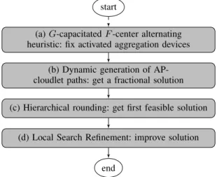
As reported in the Introduction, we found adaptations of heuristics from the literature to be unable to produce accurate results; this was one of the main motivations to build our models. Still, our path-based formulations offer great modeling flexibility and present computational challenges at once. In particular, the number of feasible paths in setsSsk andQk0k00 grows very fast with the network size. In order to obtain good feasible solutions in limited computing time, we implemented two ILP-based heuristics, whose flowcharts are presented in Fig. 2 and 3, respectively for SP and DP variants. Both heuristics share the following pre-processing steps (in Fig. 2-Block (a) and Fig. 3-2-Block (a)):
1) we fix the location of aggregation nodes, and the as-signment of APs to them, creating clusters of APs of limited size and minimum worst-case latency through the following heuristic: (i) fix a numberFof aggregation nodes to be installed; (ii) fix a maximum numberG of APs connected to each aggregation node; (iii) run a PAM k-medoids heuristic [30] on the set of APs to chooseF baricentric ones; (iv) use such a solution as initialization for aG-capacitatedF-center alternating heuristic. This alternating heuristic, in turn, works as follows: (i) fix the locations of aggregation nodes, and solve an ILP for assigning the APs to aggregation nodes, forming clusters where at most G APs are connected, and minimizing the maximum distance between an AP and the center of its cluster; (ii) choose as new center for each cluster the AP minimizing the maximum distance between all other APs in the cluster; then iterate from (i), until no more changes in the solution are observed.
2) we fix the xi variables in our models according to the G-capacitated F-center solution obtained as above, we fix J =K ={i∈ I : xi = 1}, and we remove from eachSskset all paths in which the APsis not assigned to the aggregation device of its cluster. After preliminary experiments, we fixedF = 50,G= 1.3·(|B|/F). The subsequent steps differ for the SP and DP variants, hence we present them separately.
a) Static Planning Heuristic Algorithm: The number of
feasible paths that can link APs and cloudlets can be significant and become intractable with the increase of the nodes in the network. As second step, in Figure 2-Block (b), we consider the dynamic generation of these feasible paths and their related variables rs,k
p with a so-called column generation approach
start
(a)G-capacitatedF-center alternating heuristic: fix activated aggregation devices
(b) Dynamic generation of AP-cloudlet paths: get a fractional solution (c) Hierarchical rounding: get first feasible solution
(d) Local Search Refinement: improve solution
end
Fig. 2: Structure of the Static Planning algorithm
[8]. Each Ssk is replaced by a restricted subset S˜sk having tractable size. Then, iteratively, the continuous relaxation of the model described by (1)–(23) is optimized, but including
˜
Ssk instead of Ssk, and a search for potentially improving variables in S˜sk \ Ssk is carried out. Linear programming theory guarantees that potentially improving variables are those of negative “reduced cost”: if no such a variable is found, then the solution is optimal also for the continuous relaxation of the initial model including the full sets Ssk. If, instead, variables are found having negative reduced cost, these are added to theS˜sk, and the process is iterated. In our case, the search for variables of minimum reduced cost can be formulated as a constrained shortest path problem of poly-nomial complexity, and solved with dynamic programming. Preliminary experiments proved this approach to be efficient in terms of both computing time and memory usage [31].
As the column generation process leads to a fractional solution s, to obtain an integer feasible one, a hierarchical¯
rounding on the variables is executed (Fig. 2-Block (c)): (i) select the location variable f¯ with higher fractional value in s¯ that was not already fixed, and fix it to value one, (ii) propagate the rounding, by fixing to zero all variables that would lead to infeasibility when set to one, (iii) resume column generation, to dynamically generate new paths given the new fixed variables, (iv) if a new fractional solution is found, repeat rounding from step (i); instead, if no feasible solution can be found after fixing, reset f¯ to value zero, undo rounding propagation and resume column generation; if a feasible solution is found, repeat rounding from step (i), otherwise stop rounding with FAIL. (v) Stop with SUCCESS whenever f¯has a fractional value in s¯that is lower than a small enough positive threshold .
Instead of choosing an arbitrary f¯, we perform rounding according to the following hierarchy: (i) cloudlet location vari-ableszk, (ii) core nodes location variablesyj, (iii) aggregation nodes location variables xi, (iv) paths variablesrps,k. That is, each hierarchical level is explored only if no previous one contains a fractional variable. Variables related to topological rules are never rounded explicitly. At the end of the rounding process, in case of SUCCESS, a MILP problem remains to
fix them, involving a small number of variables, which can be easily optimized by general purpose ILP solvers. Nevertheless, we often observed network topology variables to take integer values directly after rounding: in these cases we skip this last MILP optimization process. In case of FAIL, instead, the solution produced in step (a) is considered. That is, in any case our static planning algorithm produces a feasible solution, unless the instance itself admits no feasible one.
Given an integer solution S, we try to improve it withˆ an ILP-based very large scale neighborhood search strategy (Fig. 2-Block (d)), exploring aκ-OPT neighborhood [32]:
(i) we consider only the paths created during the column generation process and the subsequent hierarchical round-ing and pricround-ing;
(ii) we include the following local-branching constraint
X k∈K|¯zk=1 (1−zk) + X k∈K|¯zk=0 zk ≤ dκ· X k∈K ¯ zke (39)
wherez¯k are the fixed values of corresponding variables zk inS, andˆ κis the fraction ofzkvariables whose values are allowed to flip w.r.t. the current solution;
(iii) we solve this restricted model with a general purpose ILP Solver, setting a limit τ on the execution time.
After preliminary experiments, we set = 10−3,κ= 30%
andτ = 300seconds.
b) Dynamic Planning Heuristic Algorithm: Optimizing
the DP variant is even more involved. First, a copy of each association path rs,k,t
p needs to be considered for each time-frame t. Second, the set of sync-paths variables qpk0,k00,t may grow combinatorially as well. Third, the number of variables gks00,s,k0000 and constraints (31) - (33) is polynomial, but too large
to be explicitly considered in practice. Therefore we perform column generation also on the set of sync-paths variables, and we relax constraints (31) - (33) as follows:
X q∈Qk0,k00 qkp0,k00t≥ X s0∈B s00∈B Φ(fs0,s00)·(vs0k0+vs00k00−1) ∀k0,k00∈K |k06=k00 ∀t∈T (40) When integrality conditions are enforced, (40) are equiva-lent to (31) - (33). Unfortunately, this is not always true when the continuous relaxations are considered during rounding; we therefore strengthened them with the following inequalities:
vs0,k0+vs00,k00≤1 , ∀s 0,s00∈B k0,k00∈K | fs0,s00>0 ∃p∈Ss,k ∃p∈Ss0,k0 6∃p∈Qk0,k00 , ∀t∈T (41) vs0,k0− X k00∈K | ∃p∈Ss00,k00 ∃p∈Qk0,k00 vs00,k00≤0 , ∀s 0,s00 ∈B ∀k0∈K| fs0,s00>0∧ ∃p∈Ss0,k0 (42) X t∈T X p∈Ss,k rps,k,t≥vsk ∀s∈B,∀k∈K (43) start
(a)G-capacitatedF-center alternating heuristic (b) Dynamic generation of paths (c) Hierarchical rounding (d) Comply sync-traffic?
(e) Fix active cloudlets and APs-cloudlets associations (f) Dynamic generation of paths (g) Hierarchical rounding end No Yes 1ststage: Relaxed Synchronization Constraints 2ndstage: Generate Sync-Paths
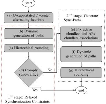
Fig. 3: Overall structure of the Dynamic Planning algorithm
where (41) forbid the simultaneous choice of AP-cloudlet associations that does not allow to establish a feasible syn-chronization path, (42) states that, for each pair of APs with expected users migration, at least a pair of AP-cloudlet associations having a feasible synchronization path has to be activated, and (43) ensure that AP-cloudlet association variable vs,kis activated only if a related path variablerps,k,tis activated in any time-framet.
The relaxed model including constraints (1)-(16), (24)-(28), (30), (34)-(36) and (40)-(43) is therefore used in the DP heuristic algorithm, whose structure is depicted in Fig. 3. Steps (b) and (c) of Fig. 3 are analogous to steps (b) and (c) of Fig. 2, but we perform the dynamic generation of both feasible associations paths rs,k,t
p and synchronization paths qkp0,k00,t. In both cases we formulated the pricing problem as a constrained shortest path problem, and we designed ad-hoc dynamic programming algorithms to solve it. At the end of the column generation, a fractional solution is available, and we resort to the hierarchical rounding to obtain an integer one. The order of rounding is the same as that used for SP variant. In fact, new continuous variablesqk0,k00t
p do not need
to be rounded; the new binary variables vs,k are not rounded explicitly but are fixed by rounding propagation: when a zk variable is fixed to zero, related vs,k variables are fixed to zero as well; when an association path variablers,k,t
p is fixed to one, the relatedvs,k variable is fixed to one as well.
At the end of the rounding process, we check the compli-ance with the relaxed constraints on synchronization traffic (31) and (33). Given the AP-cloudlet associations, defined by variables vs,k with value 1, the computation of the related amount of user migration and hence the amount of synchro-nization traffic to route is straight. If the synchrosynchro-nization paths created until this step are enough to route this amount of synchronization traffic, a feasible solution is found and
the optimization process ends successfully. If not, further synchronization paths need to be created (Fig. 3-Block (e)): we fix cloudlets locations variableszkand AP-cloudlet association variables vs,k, and the related amount of synchronization traffic is replaced in the right hand sides of constraints (40). All other variables are unfixed and a new process of dynamic generation of path variables is executed (Fig. 3-Block (f)): differently from the previous step, we look only for AP-cloudlet association paths related to variablesvs,kwhose value was fixed to one. At the end of the iterative hierarchical rounding and column generation process (Fig. 3-Block (g)), if an integer solution is found, then it is also feasible for the original problem; if not, our algorithm stops in a FAIL status. No very large scale local search is performed.
V. DATASET
In order to ground our simulations on real data, we used a dataset collected by Orange mobile, France, in the frame of the ABCD project [33]. The dataset comes from network management tickets, containing UE data exchange information aggregated in 6 minutes periods. User session is assigned to the cell identifier of the last used antenna. Data are recorded on a per-user basis and cover a large metropolitan area network, including urban, peri-urban and rural areas. We had access to data of a single 24-hour period, originated by 606 LTE 4G APs in an area of931km2, with a density of∼0.65APs per
km2. The number of users served by the considered APs is ∼180thousands, generating an overall daily traffic of11T B.
1) Estimation of Model Parameters: Coefficientsδu
s andδsb for each base stations∈B are drawn by direct queries from the dataset. Following [34] and [35] we fix costs li = 0.01, mj= 0.1, andck= 1, which can be seen as percentages. That is, we give maximum priority to the minimization of cloudlet costs, assuming to be the most relevant, and, as suggested in [34], we estimate the network costs to be as about 10% of the overall cloud data center costs.
Asdi,jvalues we take the euclidean distances between each pair of APsi, j∈B, as the underlying operator physical topol-ogy is not available to us. We recall that the topological rules we chose are described in Section III.B and encoded in set of constraints (2)-(16). We fix the bandwidth capacities u(i,j) of
each link (i, j) ∈ E to 10 Gbps in both hierarchical levels. Observing the positioning of the APs, we fix the maximum link length d¯= 7.5 km, corresponding approximately to half the radius of the metropolitan region under consideration, and we limit the paths to four hops. Instead of choosing a particular setting for C,U andD, we perform a parametric analysis on¯ them, as presented in Sect. VI.
2) User Mobility Patterns: Individual user mobility patterns
cannot be obtained for confidentiality reasons. Furthermore, allowing migrations even when an AP is visited infrequently would have a strong negative impact on the overall network load, without significantly improving user experience. Trying to cope with this issue we perform binning on data: for each user we consider his two more frequently visited APs during the planning horizon. We restrict to consider possible migrations only between these two locations representing, for
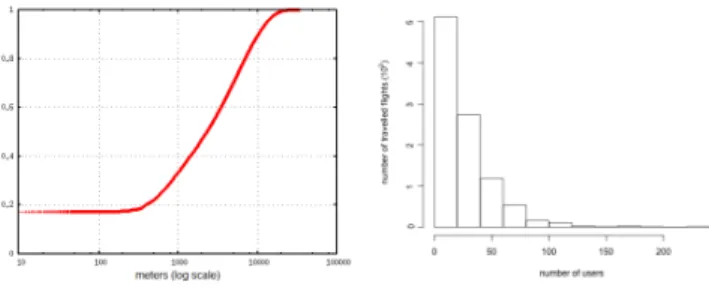
Fig. 4: CDF of traveled distances of user flights.
Fig. 5: Histogram of nb. of users covering same flight.
instance, home and work places of users, which, following [36], [37], dominate human mobility. Technically, this data is obtained by creating groups of users and obfuscating individ-ual identifiers. Other options may be considered, in absence of such data, to estimate mostly visited places [38].
Summarizing, for each pair of APs s0 ands00 let fs0,s00 be
the number of users having s0 ands00 as the most frequently visited APs; this parameter is general and can be used with any number of frequently visited locations other than two, without changes. In order to further characterize such user mobility patterns, and to allow third parties to reproduce adequately our findings, we report in Fig. 4 the cumulative distribution function of the distances traveled by users while migrating. We observe that about 20% of users do not move at all during the day and that almost all users move less than the radius of the considered region (i.e.15km). Moreover, in Fig. 5, we present a histogram reporting on thexaxis ranges for number of users. For each range [x0, x00] on the x axis, a bar represents the
number of pairs of APss0ands00 havingfs0,s00∈[x0, x00]. We
can conclude that: (i) the majority of paths are covered by a small number of users, and (ii) about 72% of the possible pairs of APs never appear as most frequent for any user. That is, the mobility is concentrated along a few frequently chosen paths, matching our intuition.
VI. EXPERIMENTALRESULTS
We implemented our algorithms in C++, using IBM ILOG CPLEX 12.6 [39] to solve both LP and MILP problems. Our experiments ran on an Intel Core 2 Duo 3Ghz workstation equipped with 2GB of RAM. In a preliminary round, we experimented on a dataset of ten small size instances involving
50 APs adapted from the facility location literature [31]. In these we could obtain valid lower bounds with our framework, measuring a worst case gap in terms of number of additional cloudlets activated in our solutions w.r.t. globally optimal ones. Our solutions were found to be of high accuracy: no extra cloudlets were activated in two cases, one extra cloudlet in seven cases and two extra cloudlets in the remaining case. That is, it was impossible to improve by removing more than a single cloudlet in nine over ten cases, even by assuming the most optimistic scenario. We experimented on the real-world dataset, considering three cloudlet size cases: tiny cloudlet of C= 2racks, car parking cloudlets ofC= 4racks andC= 5
racks, and a 2-4 DC-room cloudlet withC= 40racks. Using values from [14], we assume one rack to host up to 1500 VMs.
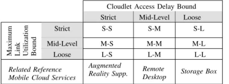
TABLE I: Labelling of parametric scenarii
Cloudlet Access Delay Bound Strict Mid-Level Loose
Maximum Link Utilization Bound
Strict S-S S-M S-L
Mid-Level M-S M-M M-L
Loose L-S L-M L-L
Related Reference Mobile Cloud Services
Augmented
Reality Supp. RemoteDesktop Storage Box
Considering bottleneck-free back-hauling networks (U ≤ 1), where latency is approximately directly proportional to the euclidean distances among nodes, we consider three la-tency bounds D: ‘loose’, ‘mid-level’, and ‘strict’ bounds,¯ corresponding respectively to roughly the urban area radius (15km),4/5of it, and2/3of it. These three levels of cloudlet access latency are chosen to correspond to three reference mobile cloud services: delay-tolerant storage box servicesfor the loose case, delay-sensitiveremote desktop servicesfor the mid-level case, and delay-critical augmented-reality support
servicesfor the strict case. We express these bounds as relative
numbers, since there is no available public information on absolute cloudlet network latency requirements, despite partial valuable information can be found at [10], [40].
As already described, the maximum link utilization ( per-centage) U needs to be kept as low as possible in order to better master the congestion risk and guarantee the QoE for real-time and interactive services. We evaluate three levels for the maximum link utilization bounds: ‘loose’, ‘mid-level’, and ‘strict’. The stricter they are, the better interactive service support is expected to be, such as for remote desktop and augmented reality. Storage box (TCP-based) services are fault tolerant, given the bulk transfer nature of its data.
In the following, we report extensive results for the SP variant, then we investigate the parametric scenarii for the DP model with VM live migration, finally comparing the approaches in terms of virtual resource migration volume with VM bulk migration. In the plots, we label every parametric scenario with a pair of letters representing respectively the maximum link utilization percentage level U and the cloudlet access latency level D, as in Table I.¯
A. Analysis of Static Planning solutions
For the static planning case (see Sect. II.B) we consider the full day average behavior, by averaging the traffic and number of users at each AP over the full day. Combining in every possible way capacity, delay and link utilization bound settings, we get3·3·3 = 27scenarii.
As first fitness measure we consider the number of installed cloudlets, as reported in Fig. 6. We can observe that:
• w.r.t. cloudlet capacity C, trivially the lowest rack ca-pacity leads to the largest number of installed cloudlets (i.e. between 15 and 20 over 50 nodes), with no relevant changes by strengthening delay and utilization bound. No substantial difference was found between the 4-rack and the 40-rack cases, while intuition suggests a lower
Fig. 6: Number of enabled cloudlets.
Fig. 7: Average usage of cloudlets (%).
number of cloudlets for the 40-rack case: this effect is due to the delay constraints requiring a minimum level of geo-distribution. Overall, intermediate size facilities (4 racks) appear as the most appealing option: smaller ones require to install on average one cloudlet every two aggregation nodes, which appears as too much, and larger ones do not reduce the number of required facilities significantly, leading to resource and space waste.
• w.r.t maximum link utilization, the number of required cloudlet facilities rapidly grows while moving from mid-level to strict bound, except for the 2-racks case, likely due to the lower aggregation of traffic on a more dis-tributed cloudlet network.
• w.r.t. cloudlet access latency, we cannot see clear trends.
On average, the solutions show little sensitivity on the value ofD, suggesting that, if a decision maker decides¯ to resort to static models unaware of users and VMs mobility, a location planning could be pursued without specifically taking into account different services. As second fitness measure, we consider the average usage of the enabled cloudlets, whose percentage values are reported in Fig. 7. Such a value is trivially related to the number of enabled cloudlets. We can however observe that:
• tiny cloudlets have always a high average usage, with a slight usage decrease just in the case with strict link utilization, having a higher number of enable cloudlets;
• 4-rack cloudlets show a behavior similar to tiny ones on mid-level and loose link utilization (scenarii M-* and L-*); on the other hand, strict constraints on link utilization (scenarii S-*) lead to a remarkable decrease of the usage;
• as expected, very big cloudlets always show little average usage, independently of other parameters choice;
• the setting of cloudlet access latency bounds has very little impact on the average cloudlet usage.
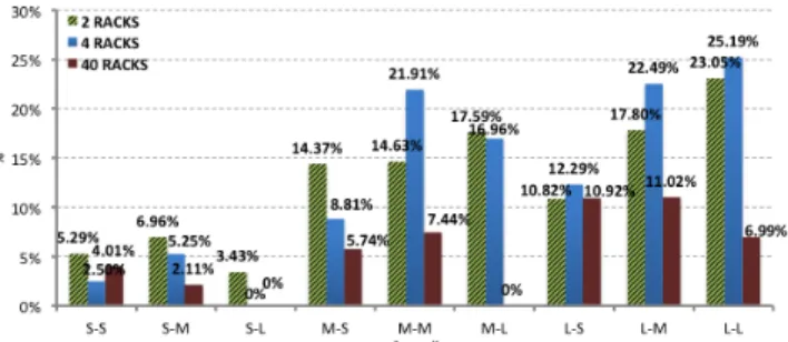
Fig. 8: Ratio of users with violated SLA after migration.
As third fitness measure, we consider the percentage of users whose SLAs are violated after their migration. In details, given a solutionS¯resulting from SP model, we know by the parameter fs0,s00 that users migrate in the planning horizon
between APss0 ands00; at the same time, we know, by values of variables rs,k
p in S, which are those cloudlets¯ k0 and k00 servicings0 ands00, respectively. If it is possible to construct, after the optimization process, a feasible synchronization path betweenk0andk00respecting constraints (32), then we say that the SLA of thosefs0,s00 users are respected; otherwise we say
that they are violated. Indeed, if a feasible synchronization path cannot be established, a user may perceive a latency during migrations that exceeds his SLA. Our results are presented in Fig. 8, where we notice that:
• enabling a high number of cloudlets leads to low percent-age of users with violated SLA: this is the case when the constraint on maximum link utilization is strict. For the scenario S-Lwe have no unsatisfied user for neither the 4-racks nor the 40-racks case;
• conversely, enabling a low number of cloudlets, the percentage of unsatisfied users increases up to25%. We argue the reason of this behavior to be the following: when the number of enabled cloudlets is high, it is possible to create a higher number of feasible synchronization paths by taking advantage of the higher number of direct links between core nodes. Indeed, the lack of control on the number of unsatisfied users in SP models is the main motivation to consider dynamic planning ones, which instead allow to explicitly enforce SLA to be never violated.
Finally, on the computational efficiency side, all SP in-stances had a running time of few minutes, with an average time of360sec., a minimum of56sec. and a maximum of821
sec., with no evident differences depending on parameters3.
B. Analysis of Dynamic Planning solutions
In a second round of experiments, we tested the behavior of the dynamic models (see Sect. III.D) in the case of two time-frames: from 7 am to 8 pm, and from 8 pm to 7 am. These approximately represent working and resting hours. We com-pared through simulations the Bulk and Live VM Migration
3Additional details on execution times are given in the Appendix Fig. A.1 of the Supplementary Materials. In Appendix A.2 of Supplementary Materials we also report additional results on the cloudlet access path length.
Summary of the parametrization of the reference mobile services can be found in the Appendix Table A.IV in Supplementary Materials.
cases. As VM replication mobility technology can be seen as a special case of VM Live Migration with infinitesimal amount of memory to transfer, we have not considered experiments using this technology; however results on VM Live Migration are valid also for VM replication scenario. Moreover we included in our tests also an SP model as reference, using data from the working-hours time-frame only (i.e. from 7 am to 8 pm). This may be seen as a ‘worst case’ planning option, since it is considering the bottleneck time-frame only; we remark that still no guarantee is obtained on SLA satisfaction, even resorting to such a conservative static option.
We restrict the simulations to the six most interesting scenarii, looking at the SP results. That is, we discard the 2-rack scenarii and the loose cloudlet access latency bound scenarii: the first proved to yield infeasible instances when the demand of the sole working-hours is considered; the second provided less interesting insights in previous analysis.
We set the width of the time window suitable to perform VM orchestration Tw to 5 hours, which is less than a half of our time-frames. For the storage synchronization path maximum length, we setD¯Q= 12.75km(4/5of the urban area radius), i.e. we consider the synchronization as a service that requires a mid-level latency bound. The size of the disk for
augmented-reality supportVMs, requiring strict latency bounds, is20GB,
reasonably lower than the one forremote desktop VMs, that is60GB, requiring mid-level latency bounds. Conversely, the size of the memory is higher for augmented-reality (8GB) than for remote desktop (4GB). To preserve tractability we defined the mapping functionΦof (33) as the following linear function that considers the synchronization traffic generated by any user as a percentageφof the average traffic generated by all users:
Φ(x) =x· P i∈I P t∈Tδ u i,t P i∈I P t∈Tδ b i,t ·φ
The percentageφis characterized by the type of mobile cloud service: considering remote desktop VMs, only part of the disk is expected to be modified upon user actions; soφis set to 70%. Instead, for augmented-reality support VMs disks are expected to be smaller and consequently only small volume need to be synchronized; soφis set to 30%3.
a) Dynamic Planning with Live Migration.: At first, we
experimented on DP variant with VM Live Migration policy. Our algorithms could find feasible solutions for 9 over 12 of these instances. In the results provided hereafter, the missing solutions are marked with the notation NF, meaning Not
Found. In fact, as our heuristic builds the solution by rounding
one variable at a time with a two-stage process, at every step there is a chance to perform a rounding that eventually leads to infeasibility. To improve this behavior a diversifica-tion mechanism could be implemented. However, since these missing results do not affect the overall understanding of our experiments, we did not further investigate in that direction.
As first fitness measure we consider the number of enabled cloudlets, reported in Fig. 9. We note that, while in the 5-rack case DP enables a slightly higher number of cloudlets w.r.t. SP, the models behave similarly in the 40-rack case.
As second fitness measure we consider the expected number of VM migrations generated by the different planning models;
Fig. 9: Number of enabled cloudlets.
Fig. 10: Expected fraction of VMs to migrate.
this can be seen as a measure of expected incremental point traffic on the network. Such a value can be computed from the values of variablesgk0k00
s0s00 that encode the number of users
moving from APs0to APs00associated to cloudletsk0andk00, resp.. We remark that in DPgk0k00
s0s00 terms are explicitly included
as variables in the models, while in SP they can be computed in a post-processing phase, once optimization is over. In order to obtain normalized fitness values, we compute the following upper bound on the number of possible VM migrations:
γ= |T| ·(|T| −1) 2 X s0∈B fs0,s0+|T|2· X s0,s00∈B|s06=s00 fs0,s00
which represents the number of migrations needed if all users are assigned to a different cloudlet in each time slot, and we measure fitness as (P
k0,k00∈B,s0,s00∈Kgk 0k00
s0s00)/γ. Our results
are reported in Fig. 10 (as percentage points).
The fraction of migrated VMs for the DP is always higher than that for the SP, without striking differences among scenarii. It is crucial to consider, however, that only DP has an explicit control on the feasibility of these orchestrations. Therefore, as third fitness measure we consider the percentage of users with violated SLA after migration (Fig. 11). DP guarantees by design 0% of users with violated SLA. On the contrary, SP, which does not give any a-priori guarantee, shows an experimental behavior similar to that presented in Fig. 8: tighter constraints on link utilization lead to a higher number of enabled cloudlets, increasing the possibility to create synchronization paths through a higher number of direct links between core nodes, and hence yielding a low fraction of unsatisfied users. A remarkable scenario is the L-S with 5-rack cloudlets: SP asks to enable 11 cloudlets, requiring
∼18% of all possible VMs migrations, but leaving∼14% of users unsatisfied; DP asks to enable, during the working-hours
Fig. 11: Percentage of users with violated SLA.
time-frame, 2 more cloudlets, requires ∼45% of all possible VMs migrations, but without violating any SLA.
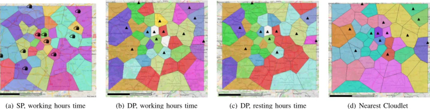
To give an insight on the reason for SLA violations in SP, we show in Fig. 12 the clusters of APs associated to the same cloudlet by: (a) SP during working-hours time-frame; (b) DP during working-hours time-frame, and (c) DP during during night-time time-frame. Cloudlet locations are identified by a triangle icon and clusters are identified by different colors. First, we observe that SP spreads cloudlets more uniformly in the region, while DP locates the cloudlets in a smaller sub-area near the center of the territory, limiting the maximum distance between two cloudlets to satisfy SLA latency bound. Second, we observe that clusters are not necessarily compact; in fact, capacity restrictions may forbid an area to be associated to its nearest cloudlet. DP tends to create a more involved clustering structure, especially during working-hours. Major changes are observed in pink and light blue clusters, while the remaining tend to keep the same structure over the two time frames.
On the computational efficiency side, while SP instances have execution times in the scale of few minutes, DP instances have execution times that ranges from few hours to several days. In particular, while SP cases have an average execution time of4min., with a minimum of74sec.and a maximum of
17 min., DP cases have and average execution time of∼22
hours, with a minimum of 75 min. and a maximum of ∼6
days. Since our model is designed for medium and long term planning, none of them appears to be critical4.
b) Nearest Cloudlet Association: In order to further
assess the need for considering the association between APs and cloudlets directly within the planning model, we propose the following experiment: given the network resulting by our model we disregard the association of AP to cloudlet, and instead we associate APs to the nearest cloudlet in terms of number of hops. For example, in Fig. 12(d) we can see the cluster of APs associated to the nearest cloudlet using the same network used in Fig. 12(b) and 12(c).
As a first comparison, in Fig. 13 we show the percentage of users with violated SLA after a nearest cloudlet association. As compared with our approach in Fig. 11, we remark that: (i) nearest cloudlet association produces SLA violations even with dynamic planning, while our approach guarantees no
4 Details on execution times are given in the Appendix Fig. A.1 in Supplementary Materials. Analysis on percentage usage of cloudlets and cumulative distribution function of the cloudlet access path lengths does not show further insight, hence we left their discussion in Appendices A.3 and A.4 in Supplementary Materials.
(a) SP, working hours time (b) DP, working hours time (c) DP, resting hours time (d) Nearest Cloudlet
Fig. 12: Clustering produced by AP-cloudlet associations in L-M scenario with 5-rack cloudlets.
Fig. 13:SLA violation (% users) with nearest cloudlet association
Fig. 14: Cloudlet overuse with nearest cloudlet association
violations; (ii) for almost all static planning scenarii, violations are worse with nearest cloudlet than with our approach.
As a second comparison, we compute the cloudlet overuse, i.e. the excess over VM capacityC. In Fig. 14 we present the overuse amount, noting that with 40-rack cloudlets there is no overuse, and with tiny 5-rack cloudlets there is a high overuse for several instances of both SP and DP approaches.
c) Bulk migration results: Our initial attempts to
op-timize DP models with VM Bulk migration produced no feasible solutions on any instance of the dataset. Indeed, bulk migration policies clash with the ambition of producing ahead a careful service and synchronization plan; in other terms, bulk migrations can be seen as the result of an unexpected need of synchronization, a human-ordered point operation, rather than a consolidated and automated operation.
Nevertheless, in order to analyze the impact of Bulk Mi-grations, we proceeded as follows. We produced solutions of DP with VM Live Migration, and we computed the maximum
size of a VM file that the network could manage to transfer without violating user SLA. Such a value is unfortunately not directly available after optimizing DP Live Migration models; on the contrary, the problem of finding it can be proved to be NP-Hard. Therefore, we performed the following simplifying assumptions: (i) cloudlets located in aggregation nodes are moved to the corresponding core nodes; (ii) synchronization paths are allowed for an arbitrary number of hops and arbitrary length - that is, synchronization is performed among core nodes only, and only maximum single-link length constraints and single-link latency bounds are kept. Assumption (i) is particularly mild, as any cloudlet placed at aggregation level would represent a bottleneck of the whole network.
The problem of finding the largest file sizeΓ turns out to be a multicommodity-flow problem modeled as follows:
max Γ (44) s.t. X k0,k00∈K fi,jk0,k00≤(1−U)·u·Tw , ∀(i, j)∈EJ (45) X j∈J fi,jk0,k00− X j∈J fj,ik0,k00= ¯ fk0k00·Γifi=k0 0ifi6=k0∧i6=k00 −f¯k0k00·Γifi=k00 ∀(k0,k00)∈K ∀i∈J (46) fi,jk0,k00= 0 , ∀(i, j)∈EJ |d(i.j)≥d¯ (47) fi,jk0,k00≥0 (48) Let:EJ be the set of links between core nodes;f¯k0k00be the
fixed number of VMs to migrate between cloudletsk0 andk00; andfi,jk0,k00 be non-negative continuous variables representing the number of VMs to migrate from k0 to k00 and whose migration path traverses link(i, j). Inequalities (47) and (45) model single-link length and latency bounds, resp.. Inequalities (46) are flow conservation constraints. That is, model (44)– (48) is a LP that can be optimized very efficiently.
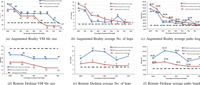
For each 5-rack cloudlets case where we obtained a feasible solution in the VM Live Migration model, we run this model with a parametric analysis on the link length threshold d:¯ starting from the value used in DP experiments, we decreased it stepwise, until the problem became infeasible.
Our results are collected in Fig. 15. Three different features of each solution are reported: (i) the optimalΓ value, i.e. the maximum VM file size that the network can afford; (ii) the av-erage number of hops of the generated synchronization paths;
and (iii) the average length of the generated synchronization paths. Each chart contains a dashed black line, representing the required standard for synchronization paths. These are 3 hops, maximum total length of 12Km and either a 28GB file (8GBmemory and20GBdisk) for the augmented reality service or a 64GB file (4GB memory and 60GB disk) for remote desktop. That is, fully feasible solutions would have values above the dashed line in the leftmost chart, and below it in the central and rightmost ones: it is easy to check that in no case it was possible to find one of them. Matching intuition, using high allowed link length values, one can move very large VM files, at the price of generating highly infeasible synchronization paths. We can further note that:
• for augmented reality reference service, using the total link length we can route very big-size VMs (almost 3 times the desired size, see Fig. 15(a)), but with highly infeasible paths (almost 3 times more hops than expected, see Fig. 15(b), and 5times longer paths, see Fig. 15(c)). However a reasonable trade-off can be reached using 75% of the maximum link length: in this case we can route a
29GBVM file, with an average number of hops of 5 and an average path length that is50% above the threshold;
• for remote desktop reference service we were not able
to route the expected VM file size (see Fig. 15(d)): a maximum file size of 29GB can be routed, and still with violations in terms of average number of hops and average paths length. No improvement is achieved by lowering the allowed link length. Moreover using less than 80% of the link length already leads to infeasibility. Summarizing, Bulk Migration seems to be a feasible al-ternative to Live Migration on Augmented Reality reference services, where the size of synchronization files is still limited; in fact solutions can be found, violating latency and maximum hop constraints only slightly. On the contrary, on Remote Desktop reference services, Bulk Migration does not appear as a viable option. In either case, matching DP models with VM Live Migration proves to be the most appealing option.
VII. CONCLUSION
We provided for the first time at the state of the art a comprehensive mobile edge cloud network design framework for mobile access metropolitan area networks. We formally defined the problem, including two planning model variations: (i) considering a static status of the network, unaware of variations during the planning horizon, and (ii) considering a dynamic network, including load variations and mobility of users and virtual machines, encoding three different virtual machine mobility technologies.
We compared the different planning options extensively for scenarii built over real cellular network datasets, differentiating between different traffic engineering and performance goals for reference mobile cloud services, analyzing: (i) the use of network facilities resources, i.e. number of enabled cloudlets, usage of cloudlet resources, migrated volume and (ii) the compliance with users’ SLA. As conclusion we can state that:
• while we guarantee full compliance with users’ SLA considering users mobility and dynamic variations of the
network, their exclusion from the modeling leads to the infringement of SLA for up to20% of users;
• the increase of use of network resources given by the
consideration of users mobility is limited to at most 5 more enabled cloudlet for serving 600 APs, for the Paris metropolitan area network use-case (on real traffic logs);
• the simultaneous consideration of the design of the net-work, the association between APs and cloudlets and the routing is needed to keep compliance with the limited resource and users’ SLA: decoupling these design deci-sions using trivial heuristics leads to SLA infringement for up to27%of users and in cloudlet capacity over-use;
• comparing VM Live Migration and VM Bulk Migration technologies, the former has proved eligible for the use both with delay-critical and delay-sensitive mobile cloud services, while the latter constantly violates limits on network resources and seems to be a feasible alternative only when the size of VM files to synchronize is small. We believe the provided insights can stimulate further re-searches in the rising research field of mobile cloud network-ing and mobile edge computnetwork-ing, especially in the field of online routing and cloud migration policies as outlined in [27], [41]. As a future work, it can be interesting to address the problem of online management of multiple VMs, application VMs and network function VMs, using multiple, possibly pre-installed, cloudlet facilities.
ACKNOWLEDGMENT
This work was partially funded by the ANR ABCD (Grant No: ANR-13-INFR-005) and the FP7 MobileCloud (Grant No. 612212) projects. We thank C. Ziemlicki and S. Uppoor from Orange for the support with cellular data retrieval.
REFERENCES
[1] A. Ceselli, M. Premoli, and S. Secci, “Cloudlet network design opti-mization,” inProc. of IFIP Networking. IEEE, 2015, pp. 1–9. [2] Cisco Systems Inc., “CVN Index: Global Mobile Data Traffic Forecast
Update, 2015–2020,” White Paper c11-520862, 2016.
[3] M. Satyanarayananet al., “The case for vm-based cloudlets in mobile computing,”IEEE pervasive Computing, vol. 8, no. 4, pp. 14–23, 2009. [4] Y. Jararwehet al., “Resource efficient mobile computing using cloudlet
infrastructure,” inProc. of IEEE MSN. IEEE, 2013, pp. 373–377. [5] “Elijah,” [Dec. 2016]. [Online]. Available: http://elijah.cs.cmu.edu [6] M. Patelet al., “Mobile-edge computing introductory technical white
paper,” ETSI, White Paper 18-09-14, 2014.
[7] A. Nealet al., “Mobile Edge Computing (MEC); Technical Require-ments,” ETSI, White Paper DGS/MEC-002TechReq, 2016.
[8] G. Desaulniers, J. Desrosiers, and M. M. Solomon,Column generation. Springer, 2006, vol. 5.
[9] S. Clinchet al., “How close is close enough? understanding the role of cloudlets in supporting display appropriation by mobile users,” inProc. of IEEE PerCom. IEEE, 2012, pp. 122–127.
[10] K. Ha et al., “The impact of mobile multimedia applications on data center consolidation,” in Cloud Engineering (IC2E), 2013 IEEE International Conference on. IEEE, 2013, pp. 166–176.
[11] D. Fesehaye et al., “Impact of cloudlets on interactive mobile cloud applications,” inEnterprise Distributed Object Computing Conference (EDOC), 2012 IEEE 16th International. IEEE, 2012, pp. 123–132. [12] Z. Panget al., “A survey of cloudlet based mobile computing,” in2015
International Conference on Cloud Computing and Big Data (CCBD). IEEE, 2015, pp. 268–275.
[13] J. Hamilton, “Architecture for modular data centers,” inInnovative Data Systems Research (CIDR), 2007 Conference on. CIDR, 2007, pp. 306– 313.