Working Paper 06-13(03)
Statistics and Econometrics Series
Febrero 2006
Departamento de Estadística
Universidad Carlos III de Madrid
Calle Madrid, 126
28903 Getafe (Spain)
Fax (34) 91 624-98-49
A TWO FACTOR LONG MEMORY STOCHASTIC VOLATILITY MODEL1
Helena Veiga2
Abstract
In this paper we fit the main features of financial returns by means of a two factor long
memory stochastic volatility model (2FLMSV). Volatility, which is not observable, is
explained by both a short-run and a long-run factor. The first factor follows a stationary
AR(1) process whereas the second one, whose purpose is to fit the persistence of
volatility observable in data, is a fractional integrated process as proposed by Breidt et
al. (1998) and Harvey (1998). We show formally that this model (1) creates more
kurtosis than the long memory stochastic volatility (LMSV) of Breidt et al. (1998) and
Harvey (1998), (2) deals with volatility persistence and (3) produces small first order
autocorrelations of squared observations. In the empirical analysis, we use the
estimation procedure of Gallant and Tauchen (1996), the Efficient Method of Moments
(EMM), and we provide evidence that our specification performs better than the LMSV
model in capturing the empirical facts of data.
Keywords:
Two Volatility Factors, Long Memory, Fractional Integration, EMM,
Reprojection.
1
I thank Michael Creel for introducing me to the idea of Efficient Method of Moments and for his constant advice. I am grateful to George Tauchen for his helpful remarks during my stay at Duke University. I also thank Esther Ruiz and seminar participants at the Universidad Complutense for their valuable comments. This research has been made possible thanks to the financial support of Fundaçao para a Ciência e Tecnologia. The usual disclaimer applies.
A Two Factor Long Memory Stochastic
Volatility Model
Helena Veiga
∗ Statistics Department, Universidad Carlos III de Madrid, C/ Madrid 126, 28903 Getafe (Madrid), Spain.E-mail: [email protected]
Abstract
In this paper wefit the main features offinancial returns by means of a two factor long memory stochastic volatility model (2FLMSV). Volatility, which is not observable, is explained by both a short-run and a long-run factor. Thefirst factor follows a stationary AR(1) process whereas the sec-ond one, whose purpose is tofit the persistence of volatility observable in data, is a fractional integrated process as proposed by Breidt et al. (1998) and Harvey (1998). We show formally that this model (1) creates more kurtosis than the long memory stochastic volatility (LMSV) of Breidt et al. (1998) and Harvey (1998), (2) deals with volatility persistence and (3) produces small first order autocorrelations of squared observations. In the empirical analysis, we use the estimation procedure of Gallant and Tauchen (1996), the Efficient Method of Moments (EMM), and we provide evidence that our specification performs better than the LMSV model in capturing the empirical facts of data.
Keywords: Two Volatility Factors, Long Memory, Fractional Integration,
EMM, Reprojection.
JEL Classification: C14.
1
Introduction
The most important feature of the conditional return distribution is its second moment dynamics. This fact has led to an enormous literature on the modelling
∗I thank Michael Creel for introducing me to the idea of Efficient Method of Moments and
for his constant advice. I am grateful to George Tauchen for his helpful remarks during my stay at Duke University. I also thank Esther Ruiz and seminar participants at the Universidad Complutense for their valuable comments. This research has been made possible thanks to thefinancial support of Fundaç˜ao para a Ciência e Tecnologia. The usual disclaimer applies.
of return volatility that had as its starting point the ARCH model of Engle (1982). The main aim of this model was tofit volatility clustering and the fat tails of the return distributions. Posteriori models were able to deal with more complex features of financial time series data, e.g. the asymmetric responses of volatility to shocks and the persistence of volatility processes. With respect to the persistence of volatility Ding et al. (1993), de Lima and Crato (1994), and Bollerslev and Mikkelsen (1996) suggested that volatility could be model as a fractional integrated process. The existence of a fractional root in the volatility process would generate more persistence and consequently lead to autocorrelation functions of squared returns that decay slowly towards zero. In the light of this finding, Breidt et al. (1998) and Harvey (1998) proposed a new time series representation of persistence in conditional volatility denoted long memory stochastic volatility model (LMSV). The LMSV incorporates an ARFIMA process in a standard stochastic volatility scheme.
In this paper, we model volatility persistence by assuming that the volatility of asset returns shows a long memory feature captured by a fractionally inte-grated process as in Breidt et al. (1998) and Harvey (1998). We also incorporate a short-run factor into the volatility specification. This factor helps to generate extra kurtosis, to accommodate the volatility persistence and to obtain small values for the first-order autocorrelation of squared returns. The introduction of this extra volatility factor is justified by the results of Andersen et al. (2002), Chernov and Ghysels (2000), Chernov et al. (2003), Eraker et al. (2003), Gal-lant and Tauchen (2001), Jones (2003), Merville and Pieptea (1989) and Pan (2002). These authors found that stochastic volatility models with one volatility factor are not able to characterize all moments of asset return distributions. In particular, the fat tails of the return distribution are captured rather poorly. Additionally, Merville and Pieptea (1989) found that some shocks that drive volatility away from its long-term value are temporal because there is a force pulling volatility back to its long-term value. These twofindings may suggest that volatility can be decomposed into a transitory and a persistent component. More recently, the use of fractional integrated processes to generate persis-tence has been questioned. Liu (2000), Breidt et al. (1998), and Morana and Beltrati (2004) argued that persistence might be generated by a regime switch-ing model. We justify our choice based on the results of Bollerslev and Mikkelsen (1996), who proved that fractional integration was an adequate proceeding for generating persistence. Moreover, our model (denoted 2FLMSV) has further advantages. First, it is well defined in the mean square sense and consequently many of its stochastic characteristics are easy to establish. Second, it general-izes the LMSV model and inherits most of its statistical properties. Finally, it incorporates the possibility of a leverage effect by allowing for a correlation be-tween the returns and the changes in volatility, [see, Taylor (1994) and Harvey and Shephard (1996)].
In our empirical analysis, we test the performance of the 2FLMSV model by
fitting it to the returns of the S&P 500 composite index. We use the efficient method of moments (EMM) of Gallant and Tauchen (1996) because of its testing advantages and the impossibility of applying maximum likelihood estimation in
models with latent variables.1Our results evidence that the 2FLMSV modelfits volatility persistence and the fat tails of the distribution of returns better than the LMSV of Breidt et al. (1998), and Harvey (1998).
The paper is organized as follows: In the next Section, we present the models and derive the main statistical properties of the 2FLMSV model. We run a Monte Carlo experiment in section 3. Afterwards, we describe our estimation technique and report the corresponding results. Finally, we conclude. Proofs and Figures are relegated to the Appendix.
2
Long Memory Stochastic Volatility Models
2.1
The Asymmetric LMSV Model
In this Subsection we review the asymmetric LMSV model of Ruiz and Veiga (2006) and present some of its most important statistical properties. This model is an extension of the LMSV specification of Breidt et al. (1998) and Harvey (1998). Formally, let the return of afinancial asset at timet, yt, satisfy
yt=σtεt, where σt=σexp(h1t/2). (1)
In equation 1,σdenotes a scale parameter,σ2t is the conditional variance ofyt,
εtis N ID(0,1)and h1t is a fractional integrated Gaussian noise process given
by
(1−L)dh1t= t and t∼N ID(0, σ2). (2)
In equation 2, L stands for the lag operator, d is the parameter of fractional integration andh1 is an unobservable latent variable that is weakly stationary
in the range d ∈ (0,0.5). Hosking (1981) showed that h1t has the following
M A(∞)representation ford <0.5: h1t= (1−L)−d t= ∞ X k=0 ψk t−k,
where ψk = Γ(Γd()kΓ+(kd+1)) and Γ(·) is the Gamma function. Observe that the coefficientsψk converge hyperbolically to zero.2
1Further estimation techniques are the procedure based on a spectral regression proposed by Geweke and Porter-Hudak (1983) and a frequency-domain estimator for the fractionally integrated stochastic volatility model (LMSV) suggested by Breidt et al. (1998). The latter estimator is consistent but the asymptotic distribution is not known. Wright (1999) proposed a new estimator for the LMSV model based on the minimum distance estimator (MDE) proposed by Tieslau et al. (1996). It consists of minimizing a quadratic distance function and estimates autocorrelations at various lags. The estimator is√T-consistent and asymptotically normal, provided that the parameter of fractional integration is smaller than 0.25.
2Ford >
−1the binomial expansion of(1−L)dis given by:(1−L)d= S∞ k=0 d k (−L)k= 1−dL−d(12!−d)L 2 −d(1−d3!)(2−d)L 3
−.... Remember thatkΓΓ((ab++xx))l≈xa−b.So, whenk→ ∞,
ψk≈ k
d−1
Ruiz and Veiga (2006) assumed additionally that (εt, t+1)0 follow the
bi-variate normal distribution µ εt t+1 ¶ ∼ N ID µµ 0 0 ¶ , µ 1 δσ δσ σ2 ¶¶ , (3)
whereδ, the correlation betweenεtand t+1, induces correlation between returns
and changes in volatility, [see, Taylor (1994) and Harvey and Shephard (1996)]. Therefore, if δ = 0, the model simplifies to the LMSV specification of Breidt et al. (1998) and Harvey (1998). Moreover, note that the series of returns is a martingale difference and, consequently, an uncorrelated sequence.
Another interesting point is the behavior of theh1tautocorrelation function
(ACF). Baillie et al. (1996) computed the moments ofh1tfrom the properties
of the lognormal distribution and obtained fork≥1the following results: σ2h1=σ2 Γ(1−2d) [Γ(1−d)]2, γ(k)≡cov(h1t, h1t+k) =σ2 Γ(1−2d)Γ(k+d) Γ(d)Γ(1−d)Γ(k+ 1−d) and ρ(k)≡corr(h1t, h1t+k) = Γ(1−d)Γ(k+d) Γ(d)Γ(k+ 1−d) = Y 1≤i≤k i+d−1 i−d .
Note that ρ(k) can be written as ρ(k) ≈ Γ(1Γ(−d)d)k2d−1 as k → ∞. Since the
autocorrelation function decays hyperbolically towards zero, the effect of a shock to volatility takes time to dissipate. This property of volatility is called long memory.3
Ruiz and Veiga (2006) derived the variance and the autocorrelation functions ofy2
t for the case whenytfollows an asymmetric LMSV model, e.g. equations
1 to 3. They obtained fork≥1that
var(y2t) =σ4exp(σ2h1)[Kεexp
¡ σ2h1¢−1] and corr(yt2, y2t+k) =exp ¡ σ2 h1ρ(k) ¢ ¡ 1 +δ2σ2ψ2 k−1 ¢ −1 Kεexp(σ2h1)−1 ,
where Kε is the kurtosis of εt. Furthermore, the excess of kurtosis of yt was
shown to be equal toEK= 3[exp(σ2
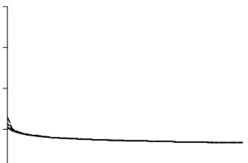
h1)−1]. Figure 1 reports the autocorrelation 3We can say that a processy
tdisplays long memory if its spectrumf(λ)has the following
asymptotic decay: f(λ)≈C(λ)|λ|−2dasλ→0+ wheneverd6= 0andC(λ)6= 0. Ifd >0,
then the autocorrelations are not summable, i.e lim n→∞
Sn
k=−∞|ρ(k)|=∞, and the spectrum
diverges at0, [see, Breidt et al. (1998)]. Brockwell and Davies (1991) and Beran (1994) pro-vided a more restrictive definition of long-memory that is more suitable forARF IM A(p, d, q) processes.
functions ofy2t for two LMSV processes until lag 50. We observe that processes
with largerd’s are simultaneously able to generate more persistence and capture more kurtosis.
2.2
The Asymmetric 2FLMSV Model
We propose a long memory stochastic volatility model with two volatility factors. It is denoted 2FLMSV. The objective of thefirst factor is to capture persistence in volatility and is similar in spirit to Breidt et al. (1998) and Harvey (1998)’s volatility process. The second factor accommodates the short run dynamics and helps generating extra kurtosis. Formally, we have now that
yt=εtσexp µ h1t+h2t 2 ¶ , (4)
where εt is again N ID(0,1). As before, σ is a scale parameter. The
frac-tional integrated processh1tis the same as in the base model and thus given by
equation 2. Moreover, we assume thath2t follows the following AR(1) process:
h2t=φh2t−1+ηt, (5)
where ηt∼N ID(0, ση2)and|φ|<1. The last condition guarantees the
station-arity of the process. The errorsηt, tandεtare contemporaneously independent
for alltand it is assumed thath1andh2are unobservable latent variables.
Fi-nally,(εt, t+1)0 follow the bivariate normal distribution presented in equation
3. Hence, the 2FLMSV model is fully specified by the set of equations 4, 2, 5 and 3.
Next, we derive closed form expressions for the main moments and the au-tocorrelation functions ofy2
t and|yt|in order to gain insights about the model’s
ability to capture the empirical dynamics of the returns distribution. In partic-ular, we are interested in the second moment, because it turned out to be the dominant time varying feature of the return distribution.
Proposition 1 In the 2FLMSV model, thefirst, the second and the fourth
un-conditional moment ofy2
t exist and have the following form:
E¡y2t¢=σ2exp à σ2 h1+σ 2 h2 2 ! , E¡yt4 ¢ =σ4Kεexp £ 2¡σ2h1+σ 2 h2 ¢¤ and
var(y2t) =σ4exp(σ2h1+σ2h2)[Kεexp(σ2h1+σ 2
h2)−1].
Proof. See the Appendix.
It is easy to obtain from Proposition 1 a closed-form expression for the excess of kurtosis ofyt. It is equal to
EK= 3[exp(σ2
h1+σ 2
A direct consequence of this result is that the 2FLMSV model is able to generate higher kurtosis than the LMSV of Breidt et al. (1998) and Harvey (1998). Next, we calculate the autocorrelation function ofy2
t.
Proposition 2 Fork ≥1, the autocorrelation function of y2
t in the 2FLMSV model is given by corr(y2t, y2t+k) = exp³σ2 h1ρ(k) +σ 2 h2φ k´ ¡ 1 +δ2σ2ψ2 k−1 ¢ −1 Kεexp ¡ σ2 h1+σ2h2 ¢ −1 .
Proof. See the Appendix.
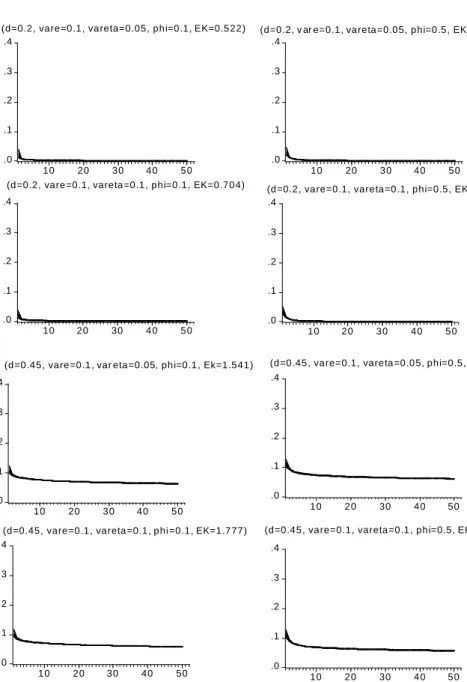
Figure 2 reports the autocorrelation functions of y2
t for several 2FLMSV
processes. We observe that the 2FLMSV model generates extra kurtosis in comparison to the LMSV (e.g. if we compare the first panel of Figure 1 with the first four panels in Figure 2, then we see that the excess of kurto-sis increased from 0.348 to at least 0.522). Additionally, we see that both models perform equally well in capturing persistence and that the 2FLMSV model creates smaller first order autocorrelations for some parameter values (©d= 0.45, σ2= 0.1, σ2 η= 0.1, φ= 0.1 ª and©d= 0.45, σ2= 0.05, σ2 η, φ= 0.1 ª ).
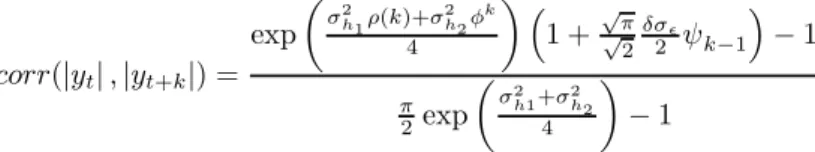
Proposition 3 Fork≥1, the k-th order autocorrelation of|yt|in the 2FLMSV
model is given by corr(|yt|,|yt+k|) = exp µ σ2h1ρ(k)+σ 2 h2φ k 4 ¶ ³ 1 +√√π 2 δσ 2 ψk−1 ´ −1 π 2exp µ σ2 h1+σ2h2 4 ¶ −1 .
Proof. See the Appendix.
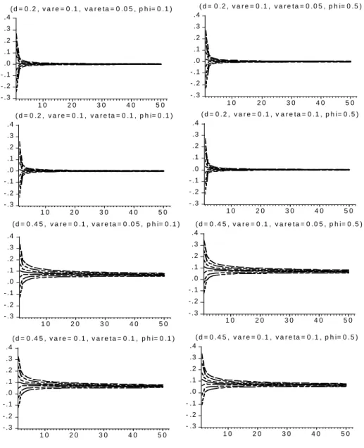
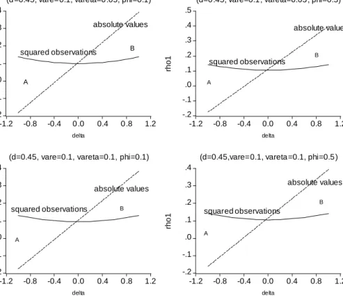
One empirical evidence of the ACF of the S&P 500 squared returns presented in Figure 7 is that the first order autocorrelation is smaller than the second order autocorrelation. Looking at Figure 3, we observe that the introduction of negative asymmetry leads the model to replicate this feature [see, e.g. the last four panels when δ=−0.2]. Finally, Figure 4 shows the relationship between thefirst order autocorrelations of absolute and squared returns. The difference between the two is known as Taylor effect. When the correlation between the level and volatility noises is positive, i.e. δ > 0, the Taylor effect is stronger for higher values ofδ. This corresponds to area B in Figure 3. On the other hand, ifδ <0, the Taylor effect disappears and the corr(|yt|,|yt+1|)is always
smaller thancorr(y2
t, yt2+1). Note that ifδ= 0, then there is no asymmetry in
the model.
3
A Monte Carlo Experiment
In this Section, we simulate several 2FLMSV processes with parameter values that reproduce the properties of real series of daily financial returns. For this
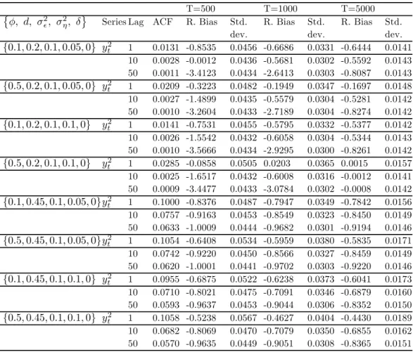
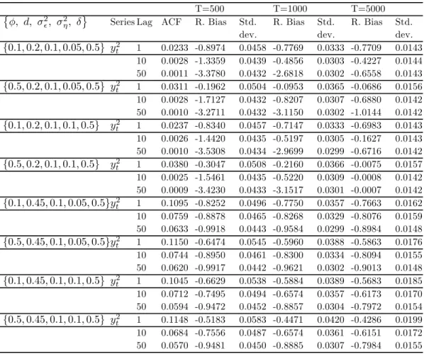
purpose, we generate1000replicates of sizeT = 500,1000and 5000. Tables 1 and 2 report the empirical relative biases and standard deviations of the sample autocorrelations of squared returns for lagsk = 1,10 and 50. For the major-ity of models the relative biases are severe. They are extremely severe for the autocorrelation of order 50 in models whose parameter d is 0.2. We also ob-serve that these biases decrease dramatically with the sample size. The same happens with the Monte Carlo standard deviations. The best fits occur for models with the parameters values ©φ, d, σ2, σ2
η, δ
ª
={0.5,0.2,0.1,0.1,0.5}
and{0.5,0.2,0.1,0.1,0.5}and with a sample size ofT = 5000. The existence of these biases may increase the difficulty of identifying long memory as it was ar-gued by Peréz and Ruiz (2003). Finally, we also observe that the autocorrelation functions (in particular, thefirst order autocorrelations of squared observations) are in majority smaller than the respective theoretical values. Peréz and Ruiz (2003) found similar evidence for LMSV models.
4
Empirical Example
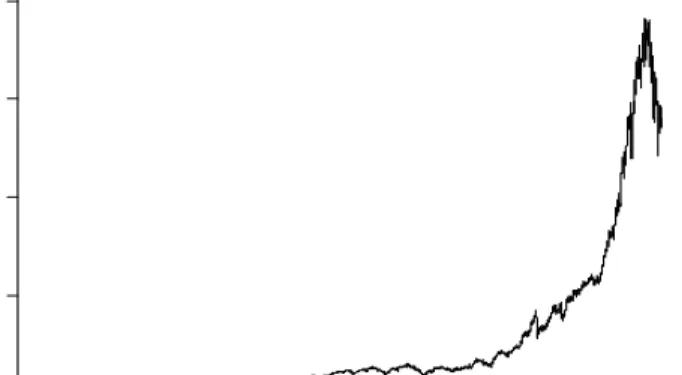
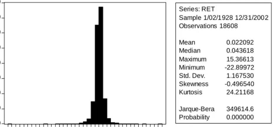
In this Section, we evaluate the performance of our model in capturing the empirical features offinancial data. We use daily close price data on the S&P 500 composite index from January 3, 1928 to February 19, 2002. This makes up to a total of 18 609 observations.
Figure 5 plots the price level and the returns on the index (adjusted for dividends and splits) over the sample period. Figure 6 provides some summary statistics of the data. The average return is 0.022 per day and the daily variance is 1.3631. Moreover, the distribution of returns is negatively skewed and the kurtosis is also quite high.
Finally, we compute the correlograms of squared and absolute returns series (Figure 7). We verify that the autocorrelation function of squared observations converges faster towards zero than the autocorrelation function of absolute re-turns. Finally, we also observe thatρ(1)is smaller thanρ(2)in both cases.
4.1
Detecting Long Memory
In order to justify our suspicion that volatility follows a fractional integrated process, we use two main tests. The first one is the traditional R/S statistic corrected for short-memory components, [see, Lo (1991)]. The second one is a Wald type test in the time domain similar to the Dickey-Fuller approach, [see, Dolado et al. (2002)].
Table 3 reports the results of the R/S test. Since the relation between J and d is given by J = d+ 1/2, [see, Mandelbrot and Taqqu (1979)] and the estimated value of J,Jb, is larger than 0.5, we conclude that the parameter of fractional integrationdis strictly positive.
Dolado et al. (2002) tested the null hypothesis of a fractional integrated process of orderd0, F I(d0), versus a fractional integrated process of order d1,
∆d1y
t−1 in a regression of ∆d0yt on ∆d1yt−1 and some lags of ∆d0yt. In our
case, we consider two different null hypotheses: d0 = 0.3 and d0 = 0.4. The
t-statistics are normally distributed because the process is stationary under the null hypothesis. The parameter d1 is estimated by fitting an ARFIMA(1,d,0)
to the squared returns series. Fractional integration is not rejected at the 5% significance level for the squared returns [see, Table 4].
4.2
E
ffi
cient Method of Moments (EMM)
Now, we estimate the LMSV and the 2FLMSV models using EMM of Gallant and Tauchen (1996). EMM is based on two compulsory phases: Thefirst phase (Projection) consists of projecting the observed data onto a transition density that is a good approximation of the distribution implicit in the true data gener-ating process. The simulated density is denominated the auxiliary model and its score is called"the score generator for EMM". The advantage of this method is that the score has an analytical expression. In the projection step, we proceed carefully along an expansion path with tree structure and the selected model comes out to be a semiparametric ARCH (auxiliar model), as in Gallant et al. (1997).4In the second phase the parameters of the models are estimated with
the help of the score generator. This score enters the moment conditions in which we replace the parameters of the auxiliary model by their quasi-MLEs obtained in the projection step. Then, the estimates of the proposed models are obtained by minimizing the GMM criterion function. Finally, EMM provides us diagnostic tests that explain the reasons for the failure or success of a model.
4.3
Empirical Results
We start by estimating the benchmark model, the LMSV model of Breidt et al. (1998) and Harvey (1998). The estimated specification is a sightly modified version of the model presented in Subsection 2.1. Following Gallant et al. (1997) we have that
yt−μy =c1(yt−1−μy) +c2(yt−2−μy) +ryεtexp(h1t/2),
and
(1−L)dh1t=rh1eεt.
At this instance, we suppose that errors are Gaussian; that is,εtisN ID(0,1),eεt
isN ID(0,1),h1tis stationary andεtandeεtare mutually independent for allt.
The change in errors notation helps detecting which parameters are separately
4The score generator is the semiparametric density (SNP) proposed by Gallant and Tauchen (1989) with the following tunning parameters: Lu = 2, which means two lags in
the linear part of the SNP model,Lr= 28that corresponds to twenty eight lags in the ARCH
part,Lp = 1, one lag in the polynomial part andfinallyKz = 8, which corresponds to a
polynomial part of degree 4 inz. Therefore, the selected auxiliary model is a semiparametric ARCH that accounts for the full complexity of the data.
identified and the parallelism is easy to establish sincerh1eεtcorresponds to t,
in our previous notation. We also introduce two lags of the dependent variable because time-series are usually correlated. Finally,μy denotes the mean ofyt.
We use the same estimation procedure of Gallant et al. (1997). Since the fractional integrated process of equation 2 can be written as a moving average of infinite order for|d|<0.5, that is
h1t= (1−L)−d t= ∞ X k=0 ψk t−k with ψk = Γ(k+d) Γ(d)Γ(k+ 1),
and the Cholesky factorization of the covariance matrix of h1t is impossible
to compute, we truncate the infinite moving average and trim off thefirst 10 000 realizations. Consequently, due to this truncation procedure, the generated process is going to be stationary for |d| < 1 but, it is still able to generate high volatility persistence, [as it has been argued by Bollerslev and Mikkelsen (1996)].
Table 5 reports the results of the specification test: the null hypothesis of correct specification is sharply rejected. Looking at the EMM quasi-t-ratiosTcn
plotted in Figure 8 we observe that the model has difficulties in matching the features of the polynomial part of the SNP score (a20 until a90). This means
that either the specification exp(h1t/2)is incorrect and/or εt is not Gaussian.
We also observe that the scores of the ARCH specification (r24 until r28) are
higger than 2. This may indicate that the conditional variance is poorlyfitted. Since the exponential transformation does not seem to be a problem in Gal-lant et al. (1997), we apply a spline error transformation to the Gaussian innovation in order to improve thefit of the polynomial part of the SNP score. The model becomes,
yt−μy =c1(yt−1−μy) +c2(yt−2−μy) +ryεtexp(h1t/2), εt=Tz(zt), Tz(zt) =bz0(bc, bd) +bz1(bc, bd)zt+bz2(bc, bd)zt2+bz3(bc, bd)ztmax(0, zt) and (1−L)dh 1t=rh1eεt.
Liu (2000) definedbz0, bz1, bz2 andbz3 as functions ofbc and bd such that ifbc
andbdare equal to 0,bz0=bz2=bz3= 0andbz1= 1. Moreover, he usedbz0= (bc+ 0.5bd)/s,bz1= 1/s,bz2=bc/sandbz3=bd/s, wheres= (bc+ 0.5bd)2+
1+3b2
c+1.5b2d+2 [(bc+ 0.5bd)bc+ 0.5 (bc+ 0.5bd)bd+ 0.7979bd+ 1.5bdbc]. These
restrictions on theb’s allow to identify all the parameters of the model and make the expected value ofTz(z)and its variance to be 0 and 1, respectively.
Table 6 and Figure 8 reveal that this change reduces the value of the EMM objective function. The moments of the polynomial part of the SNP score are now better fitted. Although there is an improvement, the model is still not able to fit all the kurtosis of data. With respect to the scores of the ARCH
specification, we encounter the same problem as before and therefore the idea of a possible misspecification in the conditional variance process is reenforced.
We have proved in Subsection 2.2 that the introduction of an extra volatility factor allows the model to generate extra kurtosis. Having in mind this purpose, we estimate the following specifications
yt−μy=c1(yt−1−μy) +c2(yt−2−μy) +ryεtexp¡h1t+2h2t¢, εt=Tz(zt), Tz(zt) =bz0(bc, bd) +bz1(bc, bd)zt+bz2(bc, bd)zt2+bz3(bc, bd)ztmax(0, zt), (1−L)dh 1t=rh1(eεt+δεt−1), withδ= 0andδ6= 0 and h2t=φ1h2t−1+φ2h2t−2+rh2eεt.
We impose the same restrictions as before to the spline error,Tz(zt)in order to
identify the parameters of the model.
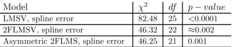
The empirical results for the non-asymmetric 2FLMSV model are reported in Tables 6 and 7 and Figure 9. They reveal that, (1) thefit is better, (2) the fatness of the tails are much better accommodated and (3) the model is able to deal much better with volatility persistence than the LMSV model with spline errors. Looking carefully at the quasi t-ratios we observe that the majority of them are smaller than 2 in absolute value, and therefore, the model does better than the corresponding benchmark model. Furthermore, all coefficients have the expected signs and are statistical significant at the 5% significance level. Nevertheless, we still reject the specification. Finally, we re-estimate the spline 2FLMSV specification introducing a leverage effect. In Tables 6 and 7 we observe that the fit does not improve much and that the estimate of leverage effect, δ, is not significant. This is not really a surprise, because the spline transformation introduces already an asymmetry into the model.
The fact that the 2FLMSV specification is still rejected by the specification test can be due to an over rejection problem that characterizes theχ2test.
Chu-macero (1997) studies the small sample properties of EMM estimators for the ARSV model with the help of a Monte Carlo experiment and confirms that infer-ence based on the over identifying restrictions test as well as otherχ2 statistics show important over rejections. In fact, if we compute the reprojected volatility using the reprojection technique of Gallant and Tauchen (1998)[see, Figure10]
and compare it to the one-step-ahead conditional volatility computed on the ob-served data, then we observe that the reprojected volatility closely encompasses the empirical volatility without missing the volatility cycles of S&P 500 (the initial high volatility, the period of low volatility at the middle of the sample, the stock market crash of October 1987 and the high volatility at the end of sample).5 This is important because the main role of these models is to
pro-5The reprojected volatility is calculated with the reprojection technique of Gallant and Tauchen (1998). Thus, as a by-product of the estimation step, we obtain a long simulation of
duce accurate future values of volatility that can be applied in areas such as risk management and asset pricing.
5
Conclusion
In this paper, we propose a two factor long memory stochastic volatility model (2FLMSV) as an alternative to the LMSV model of Breidt et al. (1998) and Har-vey (1998). We still model volatility persistence by assuming that the volatility of returns shows a long memory feature captured by a fractionally integrated process. The innovation is that we introduce a short run volatility factor that allows the model to generate extra kurtosis and to accommodate volatility per-sistence.
In thefirst step of our analysis, we derive the most important moments and the autocorrelation functions of squares and absolute values ofyt (ytfollows a
2FLMSV process). Afterwards, we apply the efficient method of moments of Gallant and Tauchen (1996) in order to compare the 2FLMSV empirically with the LMSV model.
Our results evidence that the short run volatility factor seems to improve the EMM criterion (a similar result was found by Liu (2000)) and that the long memory stochastic volatility model with two factors of volatility creates more kurtosis than the benchmark model.
References
[1] Andersen, T. G., Benzoni, L. and Lund, J. (2002): An Empirical Investi-gation of Continuous-Time Equity Return Models,Journal of Finance 57, 1239-1284.
[2] Baillie, R., Bollerslev, T. and Mikkelsen, H.O. (1996): Fractionally Inte-grated Generalized Autoregressive Conditional Heteroskedasticity, Journal of Econometrics 52, 91-113.
[3] Beran, J. (1994): Statistics for Long-Memory Processes, Chapman and Hal, New York.
ytat the estimated parameter vector with a simulation length equal 100 000. If we impose a
SNP-GARCH model on the simulated values ofyt(eyt), we obtain a good representation of the
one-step-ahead conditional variance that we denotedeσ2t. Therefore, regressingeσ2ton lags ofeσ2t, e
yt,|yet|, such aseσ2t=α0+α1σe2t−1+....+αpeσ2t−p+θ1yet−1+...+θqeyt−q+π1|yet−1|+...+πr|yet−r| +ut, gives us a calibrated function inside the simulation that provides predicted values of the
conditional variance. Then, if we evaluate this function on the observed data series we obtain estimates of the conditional variance,eσ∗t2.
The empirical volatility (the volatility obtained directly from the data) is computed by taking the square root of a moving average of squared residuals,[(m+ 1)−1Sm
j=0eˆ2t−j]1/2, m= 4orm= 26, from the estimation of the AR(1) modelyt=α0+α1yt−1+et, [see, Gallant
[4] Bollerslev, T. and Mikkelsen, H.O. (1996): Modeling and Pricing Long Memory in Stock Market Volatility, Journal of Econometrics 73, 151-184. [5] Breidt, F., Crato, N. and de Lima, P.J.F. (1998): On The Detection and Estimation of Long Memory in Stochastic Volatility,Journal of Economet-rics 83, 325-348.
[6] Brockwell, P.J. and Davis, R.A. (1991): Time Series: Theory and Methods, 2nd ed., Springer Verlag, Berlin.
[7] Chernov, M., Gallant, A. R., Ghysels, E. and Tauchen, G. (2003): Alter-native Models for Stock Price Dynamics, Journal of Econometrics 116, 225-257.
[8] Chernov, M. and Ghysels, E. (2000): A Study Towards a Unified Approach to the Joint Estimation of Objective and Risk Neutral Measures for the Purpose of Options Valuation, Journal of Financial Economics 56, 407-458.
[9] Chumacero, R. A. (1997): Finite Sample Properties of the Efficient Method of Moments,Studies in Nonlinear Dynamics and Econometrics 2, no 2.
[10] de Lima, P.J.F. and Crato, N. (1994): Long-Range Dependence in the Conditional Variance of Stock Returns,Economic Letters 45, 281-285. [11] Ding, Z., Engle, R.F. and Granger, C.W.J. (1993): A Long Memory
Prop-erty of Stock Market Returns and a New Model, Journal of Empirical Finance 1, 83-106.
[12] Dolado, J., Gonzalo J. and Mayoral, L. (2002): A Fractional Dickey-Fuller Test for Unit Roots, Econometrica70, 1963-2006.
[13] Engle, R.F. (1982): Autoregressive Conditional Heteroscedasticity with Es-timates of the Variance of UK Inflation,Econometrica 50, 987-1008. [14] Eraker, B., Johannes, M. and Polson, N. (2003): The Impact of Jumps in
Returns and Volatility, Journal of Finance 53, 1269-1300.
[15] Gallant, A.R., Hsieh, D. and Tauchen, G. (1997): Estimation of Stochatic Volatility Models with Diagnostics,Journal of Econometrics 81, 159-192. [16] Gallant, A. R. and Tauchen, G. (1996): Which Moments to Match,
Econo-metric Theory 12, 657-681.
[17] Gallant, A. R. and Tauchen, G. (1998): Reprojecting Partially Observed Systems with Application to Interest Rate Diffusions,Journal of the Amer-ican Statistical Association 93, 10-24.
[18] Gallant, A. R. and Tauchen, G. (2001): Efficient Method of Moments, Discussion Paper, University of North Carolina at Chapel Hill.
[19] Geweke, J. and Porter-Hudak, S. (1983): The Estimation and Application of Long-Memory Time Series Models,Journal of Time Series 4, 221-238. [20] Harvey, A. (1998): Long Memory in Stochastic Volatility, In J. Knight
and S. Satchell (eds.),Forecasting Volatility in Financial Markets.Oxford: Butterworth-Heinemann.
[21] Harvey A.C. and Shephard, N.G. (1996): Estimation of an Asymmetric Stochastic Volatility Model for Asset Returns, Journal of Business and Economic Statistics 14,429-434.
[22] Hosking, J.R.M. (1981): Fractional Differencing,Biometrika 68, 165-176. [23] Jones, C. (2003): The Dynamics of Stochastic Volatility,Journal of
Econo-metrics 116, 181-224.
[24] Liu, M. (2000): Modeling Long Memory in Stock Market Volatility,Journal of Econometrics 99,139-171.
[25] Lo, A.W. (1991): Long Term Memory in Stock Market Prices, Economet-rica 59, 1279-1313.
[26] Mandelbrot, B.B. and Taqqu, M (1979): Robust R/S Analysis of Long-Run Serial Correlation, Proceedings of the 42nd Session of the International
Statistical Institute, International Statistical Institute.
[27] Merville, L.J. and Pieptea, D.R. (1989): Stock-Price Volatility, Mean-Reverting Diffusion and Noise, Journal of Financial Economics 24, 193-214.
[28] Morana, C. and Beltratti, A. (2004): Structural Change and Long-Range Dependence in Volatility If Exchange Rates: Either, Neither of Both?, Journal of Empirical Finance 11, 629-658.
[29] Pan, J. (2002): The Jump-Risk Premia Implicit in Options: Evidence from an Integrated Time-Series Study,Journal of Financial Economics63, 3-50. [30] Pérez, A. and Ruiz, E. (2003): Properties of the Sample Autocorrelations of Nonlinear Transformations in Long-Memory Stochastic Volatility Models, Journal of Financial Econometrics 1, 420-444.
[31] Ruiz, E. and Veiga, H. (2006): Modelling Long-Memory Volatilities with Leverage Effect: A-LMSV Versus FIEGARCH, Manuscript, Universidad Carlos III de Madrid.
[32] Taylor, S.J. (1994): Modelling Stochastic Volatility: A Review and Com-parative Study,Mathematical Finance 4, 183-204.
[33] Tieslau, M.A., Schmidt, P. and Baillie, R.T. (1996): A Minimum Distance Estimator for Long-Memory Processes, Journal of Econometrics 71, 249-264.
[34] Wright, J. H. (1999): A New Estimator of the Fractionally Integrated Sto-chastic Volatility Model,Economics Letters 63, 295-303.
Appendix: Proofs
Proof of Proposition 1
(1) Taking squares in equation 4 yields y2
t = ε2tσ2exp (h1t+h2t). Now, we
apply expectations to the latter equation to obtain that E¡yt2¢=E£ε2tσ2exp (h1t+h2t)¤=σ2exp à σ2 h1+σ 2 h2 2 ! .
The last step of the former calculations follows becauseE[exp(h1t)] = exp
µ o2 h1 2 ¶ , E[exp(h2t)] = exp µ o2 h2 2 
and the processesh1tand h2tare not correlated. ¤
(2) Taking both sides of equation 4 to the power 4 and applying expectations afterwards yields
E¡yt4¢=E£εt4σ4exp(0.5(h1t+h2t))4¤=E(ε4t)σ4E[exp(2(h1t+h2t))].
Finally, since E¡ε4
t
¢
= Kε and E[exp(2(h1t+h2t))] = exp
µ 22σ2h1+σ 2 h2 2 ¶ we obtain thatE(y4t) =Kεσ4exp£2(σ2h1+σ
2
h2)
¤
. ¤
(3) We have thatvar(y2
t) =E(yt4)−E ¡ y2 t ¢2 . If we replaceE(y4 t) and E ¡ y2 t ¢ by the expressions obtained in part (1) and (2) of this proof, then we see that
var(y2 t) =σ4Kεexp£2¡σ2h1+σ 2 h2 ¢¤ −σ4exp¡σ2 h1+σ 2 h2 ¢ =σ4exp(σ2 h1+σ 2 h2)[Kεexp(σ 2 h1+σ 2 h2)−1].
This completes the proof of Proposition 1. ¤
Proof of Proposition 2
Taking squares in equation 4 yieldsy2
t =ε2tσ2exp(h1t+h2t). If we apply that
cov(y2 t, yt2+k) =E(yt2y2t+k)−E(yt2)E(yt2+k), then we obtain cov(y2 t, yt2+k) = E[εt2σ2exp(h1t+h2t)ε2t+kσ2exp(h1t+k+h2t+k)]− −E[ε2 tσ2exp(h1t+h2t)]E[ε2t+kσ2exp(h1t+k+h2t+k)].
We use part (1) of Proposition 1 to yield that cov(y2 t, y2t+k) = E[εt2σ2exp(h1t+h2t)ε2t+kσ2exp(h1t+k+h2t+k)]− −σ4exp(σ2 h1+σ 2 h2). (6)
In the next step we develop the expressionE(y2tyt2+k). We start by adding and
subtractingψk−1 t+1 to the processh1t. We obtain thatE(yt2y2t+k)is equal to
σ4E[ε2texp(h1t+h1t+k−ψk−1 t+1+ψk−1 t+1) exp(h2t+h2t+k)ε2t+k].
If we apply then thatE(ε2t+k) = 1,E[exp(h2t+h2t+k)] = exp(σ2h2+σ 2 h2φ k )and E[exp¡h1t+h1t+k−ψk−1 t+1 ¢ ] = exp(σ2 h1+σ2h1ρh1(k)−0.5ψ 2 k−1σ2), then we
can reduce the former equation to E(y2 tyt2+k) = σ4E[ε2texp(ψk−1 t+1)] exp(σ2h1+σ2h1ρh1(k)−0.5ψ 2 k−1σ2)· ·exp(σ2 h2+σ 2 h2φ k).
Now, observe that E[ε2texp(ψk−1 t+1)] = E[E(ε2t| t+1) exp(ψk−1 t+1)]. Since
the process εt| t+1 is distributed N( t+1·δ/σ ,1−δ2), we can calculate
im-mediately that E(ε2
t| t+1) = (1−δ2) + δ
2
σ2 2t+1. Consequently, the
expecta-tion E[E(ε2
t| t+1) exp(ψk−1 t+1)] has to be equal to (1−δ2) exp(ψ2k−1
σ2 2) +
δ2
σ2E[ 2t+1exp(ψk−1 t+1)]. Once we have calculated the last expectation we can
see thatE[E(ε2 t| t+1) exp(ψk−1 t+1)] = exp(ψ2k−1 σ2 2 )(1 +δ 2 σ2ψ2 k−1). We can
now replace the expectation in the original expression. As a result, we observe that E(y2 tyt2+k) = σ4exp(σ2h1+σ2h1ρh1(k)−ψ 2 k−1 σ2 2 ) exp(ψ 2 k−1 σ2 2)· ·(1 +δ2σ2ψ2k−1) exp(σ2h2+σ 2 h2φ k ). After rearranging terms we see that
E¡yt2yt2+k¢=σ4exp(σ2h1+σ2h2) exp³σh21ρh1(k) +σ 2
h2ρh2φ
k´ ¡
1 +δ2σ2ψ2k−1¢. If use the last expression in equation 6, we obtain fork>1that
cov(y2 t, yt2+k) = σ4exp(σ2h1+σ2h2) exp(σ 2 h1ρh1(k) +σ 2 h2ρh2φ k) · ·(1 +δ2σ2ψ2 k−1)−σ4exp(σ2h1+σ 2 h2) = σ4exp(σ2 h1+σ2h2)· ·[exp(σ2 h1ρh1(k) +σ 2 h2ρh2φ k)(1 +δ2σ2ψ2 k−1)−1]
Fork≥1, the autocorrelation function is then given by corr(y2t, yt2+k) = exp(σ 2 h1ρh1(k) +σ 2 h2ρh2φ k )(1 +δ2σ2ψ2 k−1)−1 Kεexp(σ2h1+σ 2 h2)−1 .
This completes the proof of Proposition 2. ¤
Proof of Proposition 3
This proof follows the very same steps as the proof of Proposition 2. Addition-ally, it is required to know that the expected value of a chi-squared variable X with v degrees of freedom to the powe a, E(Xva), and the expected value of the absolute value of random variableY ∼N(0,1)to the power b,E(|Y|b), are equal to2aΓ(a+v2)
Γ(v
2) andE(X
b/2
1 ), respectively. Using these results we obtain
after some computations that E(|yt|) =σE µ |εt|exp µ h1t+h2t 2 ¶¶ =σ √ 2 √πexp à σ2h1+σ2h2 8 ! and var(|yt|) =σ2 2 πexp à σ2h1+σ2h2 4 ! " π 2exp à σ2h1+σ2h2 4 ! −1 # .
Fork≥1, the covariance function for|yt|is computed in the same way as the one
in the proof of Proposition 2. The difference is that nowE[|εt|exp(ψk−1 t+1)] =
E[E(|εt| | t+1) exp(ψk−1 t+1)] = exp(ψ2k−1 σ2 8)( √ 2 √π+ δσ2 ψk−1). Consequently, we yield cov(|yt|,|yt+k|) =σ2 2 π+ √ 2 √πδσ2 ψk−1 exp # σ2 h1(1 +ρ(k)) +σ 2 h2(1 +φ k) 4 $ −π2 and corr(|yt|,|yt+k|) = exp µ σ2 h1ρ(k)+σ 2 h2φ k 4 ¶ ³ 1 +√√π 2 δσ 2 ψk−1 ´ −1 π 2exp µ σ2 h1+σ2h2 4 ¶ −1 .
Figures and Tables
.0 .1 .2 .3 .4 5 10 15 2 0 25 30 35 40 4 5 5 0 (d=0 .2, vare =0.1, E K =0.3 48) .0 .1 .2 .3 .4 5 10 15 2 0 25 30 35 40 4 5 5 0 (d=0 .45, vare=0 .1 , E K =1.32) Figure 1: Autocorrelations of y2t in LMSV processes. (continuous line
(δ= 0), dotted (δ= 0.2), dotted discontinuous (δ= 0.5) and discontin-uous (δ= 0.8)).
.0 .1 .2 .3 .4 10 20 30 40 50
(d=0.2, vare=0.1, vareta=0.05, phi=0.1, EK=0.522)
.0 .1 .2 .3 .4 10 20 30 40 50
(d=0.2, v ar e=0.1, vareta=0.05, phi=0.5, EK=0.579)
.0 .1 .2 .3 .4 10 20 30 40 50
(d=0.2, vare=0.1, vareta=0.1, phi=0.1, EK=0.704)
.0 .1 .2 .3 .4 10 20 30 40 50
(d=0.2, vare=0.1, vareta=0.1, phi=0.5, EK=0.826)
.0 .1 .2 .3 .4 10 20 30 40 50
(d=0.45, vare=0.1, var eta=0.05, phi=0.1, Ek=1.541)
.0 .1 .2 .3 .4 10 20 30 40 50
(d=0.45, vare=0.1, vareta=0.05, phi=0.5, EK=1.616)
.0 .1 .2 .3 .4 10 20 30 40 50
(d=0.45, vare=0.1, vareta=0.1, phi =0.1, EK=1.777)
.0 .1 .2 .3 .4 10 20 30 40 50
(d=0.45, vare=0.1, vareta=0.1, phi=0.5, EK =1.934)
Figure 2: Autocorrelations of yt2 in 2FLMSV processes. (continuous line (δ = 0), dotted (δ = 0.2), dotted discontinuous (δ = 0.5) and discontinuous (δ= 0.8)).
- . 3 - . 2 - . 1 . 0 . 1 . 2 . 3 . 4 1 0 2 0 3 0 4 0 5 0 ( d = 0 . 2 , v a r e = 0 . 1 , v a r e ta = 0 .0 5 , p h i= 0 . 1 ) - .3 - .2 - .1 .0 .1 .2 .3 .4 1 0 2 0 3 0 4 0 5 0 ( d = 0 . 2 , v a r e = 0 .1 , v a r e t a = 0 . 0 5 , p h i= 0 .5 ) - .3 - .2 - .1 .0 .1 .2 .3 .4 1 0 2 0 3 0 4 0 5 0 ( d = 0 . 2 , v a r e = 0 . 1 , v a r e ta = 0 .1 , p h i= 0 . 1 ) - . 3 - . 2 - . 1 . 0 . 1 . 2 . 3 . 4 1 0 2 0 3 0 4 0 5 0 ( d = 0 . 2 , v a r e = 0 . 1 , v a r e ta = 0 .1 , p h i= 0 . 5 ) - .3 - .2 - .1 .0 .1 .2 .3 .4 1 0 2 0 3 0 4 0 5 0 ( d = 0 .4 5 , v a r e = 0 .1 , v a r e t a = 0 . 0 5 , p h i= 0 .1 ) - . 3 - . 2 - . 1 . 0 . 1 . 2 . 3 . 4 1 0 2 0 3 0 4 0 5 0 ( d = 0 . 4 5 , v a r e = 0 .1 , v a r e t a = 0 . 0 5 , p h i= 0 .5 ) - . 3 - . 2 - . 1 . 0 . 1 . 2 . 3 . 4 1 0 2 0 3 0 4 0 5 0 ( d = 0 .4 5 , v a r e = 0 .1 , v a r e t a = 0 . 1 , p h i= 0 .1 ) - .3 - .2 - .1 .0 .1 .2 .3 .4 1 0 2 0 3 0 4 0 5 0 ( d = 0 . 4 5 , v a r e = 0 . 1 , v a r e ta = 0 . 1 , p h i= 0 . 5 )
Figure 3:Autocorrelations of|yt|in 2FLMSV processes. (continuous line
(δ= 0), dotted (δ= 0.2), dotted discontinuous (δ= 0.5), discontinuous (δ = 0.8), two dotted discontinuous (δ = −0.2), large discontinuous (δ=−0.5) and three dotted discontinuous (δ=−0.8)).
-.2 -.1 .0 .1 .2 .3 .4 -1.2 -0.8 -0.4 0.0 0.4 0.8 1.2 (d=0.45, vare=0.1, vareta=0.05, phi=0.1)
delta rh o 1 squared observations absolute values -.2 -.1 .0 .1 .2 .3 .4 .5 -1.2 -0.8 -0.4 0.0 0.4 0.8 1.2 (d=0.45, vare=0.1, vareta=0.05, phi=0.5)
delta rh o 1 squared observations absolute values A B -.2 -.1 .0 .1 .2 .3 .4 -1.2 -0.8 -0.4 0.0 0.4 0.8 1.2 (d=0.45, vare=0.1, vareta=0.1, phi=0.1)
delta rh o 1 squared observations absolute values A B -.2 -.1 .0 .1 .2 .3 .4 -1.2 -0.8 -0.4 0.0 0.4 0.8 1.2 (d=0.45,vare=0.1, vareta=0.1, phi=0.5 )
delta rh o 1 squared observations absolute values A B A B
Figure 4: The relationship between the autocorrelation of order 1 andδ
T=500 T=1000 T=5000
©
φ, d, σ2, σ2
η, δ
ª
Series Lag ACF R. Bias Std. dev. R. Bias Std. dev. R. Bias Std. dev. {0.1,0.2,0.1,0.05,0} y2 t 1 0.0131 -0.8535 0.0456 -0.6686 0.0331 -0.6444 0.0141 10 0.0028 -0.0012 0.0436 -0.5681 0.0302 -0.5592 0.0143 50 0.0011 -3.4123 0.0434 -2.6413 0.0303 -0.8087 0.0143 {0.5,0.2,0.1,0.05,0} y2 t 1 0.0209 -0.3223 0.0482 -0.1949 0.0347 -0.1697 0.0148 10 0.0027 -1.4899 0.0435 -0.5579 0.0304 -0.5281 0.0142 50 0.0010 -3.2604 0.0433 -2.7189 0.0304 -0.8274 0.0142 {0.1,0.2,0.1,0.1,0} y2 t 1 0.0141 -0.7531 0.0455 -0.5795 0.0332 -0.5377 0.0142 10 0.0026 -1.5542 0.0432 -0.6058 0.0304 -0.5344 0.0143 50 0.0010 -3.5666 0.0434 -2.9295 0.0300 -0.8261 0.0142 {0.5,0.2,0.1,0.1,0} y2 t 1 0.0285 -0.0858 0.0505 0.0203 0.0365 0.0015 0.0157 10 0.0025 -1.6517 0.0432 -0.6008 0.0316 -0.0012 0.0141 50 0.0009 -3.4477 0.0433 -3.0784 0.0302 -0.0008 0.0142 {0.1,0.45,0.1,0.05,0}y2 t 1 0.1000 -0.8376 0.0487 -0.7947 0.0349 -0.7842 0.0156 10 0.0757 -0.9163 0.0453 -0.8549 0.0323 -0.8450 0.0149 50 0.0633 -1.0009 0.0444 -0.9682 0.0301 -0.9194 0.0146 {0.5,0.45,0.1,0.05,0}y2 t 1 0.1054 -0.6408 0.0534 -0.5959 0.0380 -0.5835 0.0171 10 0.0742 -0.9220 0.0450 -0.8566 0.0327 -0.8459 0.0149 50 0.0620 -1.0001 0.0441 -0.9702 0.0303 -0.9220 0.0146 {0.1,0.45,0.1,0.1,0} y2 t 1 0.0955 -0.6875 0.0522 -0.6238 0.0373 -0.6041 0.0173 10 0.0710 -0.8021 0.0475 -0.7091 0.0346 -0.6879 0.0160 50 0.0593 -0.9637 0.0453 -0.9044 0.0306 -0.8352 0.0150 {0.5,0.45,0.1,0.1,0} y2 t 1 0.1058 -0.5238 0.0567 -0.4627 0.0404 -0.4430 0.0189 10 0.0682 -0.8069 0.0470 -0.7079 0.0350 -0.6855 0.0162 50 0.0570 -0.9635 0.0449 -0.9051 0.0308 -0.8365 0.0151
Table 1: Monte Carlofinite sample relative biases and standard devia-tions of sample autocorreladevia-tions of y2
t in 2FLMSV models together with
T=500 T=1000 T=5000
©
φ, d, σ2, σ2
η, δ
ª
Series Lag ACF R. Bias Std. dev. R. Bias Std. dev. R. Bias Std. dev. {0.1,0.2,0.1,0.05,0.5} y2 t 1 0.0233 -0.8974 0.0458 -0.7769 0.0333 -0.7709 0.0143 10 0.0028 -1.3359 0.0439 -0.4856 0.0303 -0.4227 0.0144 50 0.0011 -3.3780 0.0432 -2.6818 0.0302 -0.6558 0.0143 {0.5,0.2,0.1,0.05,0.5} y2 t 1 0.0311 -0.1962 0.0504 -0.0953 0.0365 -0.0686 0.0156 10 0.0028 -1.7127 0.0432 -0.8207 0.0307 -0.6880 0.0142 50 0.0010 -3.2711 0.0432 -3.1150 0.0302 -1.0144 0.0142 {0.1,0.2,0.1,0.1,0.5} y2 t 1 0.0237 -0.8340 0.0457 -0.7147 0.0333 -0.6983 0.0143 10 0.0026 -1.4420 0.0435 -0.5197 0.0305 -0.1627 0.0143 50 0.0010 -3.5308 0.0434 -2.9699 0.0299 -0.6716 0.0142 {0.5,0.2,0.1,0.1,0.5} y2 t 1 0.0380 -0.3047 0.0508 -0.2160 0.0366 -0.0075 0.0157 10 0.0025 -1.5461 0.0435 -0.5220 0.0309 -0.0008 0.0142 50 0.0009 -3.4230 0.0433 -3.1517 0.0301 -0.0007 0.0142 {0.1,0.45,0.1,0.05,0.5}y2 t 1 0.1095 -0.8252 0.0496 -0.7750 0.0357 -0.7663 0.0162 10 0.0759 -0.8878 0.0465 -0.8268 0.0329 -0.8076 0.0159 50 0.0633 -0.9918 0.0443 -0.9584 0.0299 -0.8984 0.0148 {0.5,0.45,0.1,0.05,0.5}y2 t 1 0.1150 -0.6474 0.0545 -0.5960 0.0388 -0.5863 0.0176 10 0.0744 -0.8950 0.0461 -0.8300 0.0334 -0.8094 0.0155 50 0.0620 -0.9917 0.0442 -0.9621 0.0302 -0.9013 0.0148 {0.1,0.45,0.1,0.1,0.5} y2 t 1 0.1045 -0.6629 0.0538 -0.5884 0.0389 -0.5683 0.0185 10 0.0712 -0.7495 0.0494 -0.6574 0.0357 -0.6173 0.0170 50 0.0594 -0.9472 0.0452 -0.8857 0.0304 -0.7972 0.0154 {0.5,0.45,0.1,0.1,0.5} y2 t 1 0.1148 -0.5183 0.0583 -0.4471 0.0420 -0.4286 0.0199 10 0.0684 -0.7556 0.0487 -0.6574 0.0361 -0.6151 0.0172 50 0.0570 -0.9481 0.0450 -0.8885 0.0307 -0.7984 0.0155
Table 2: Monte Carlofinite sample relative biases and standard devia-tions of sample autocorreladevia-tions of y2
t in 2FLMSV models together with
0 4 00 8 00 1 2 0 0 1 6 0 0 1 9 3 0 1 9 4 0 1 9 5 0 1 96 0 1 97 0 1 9 8 0 1 9 9 0 2 0 0 0 - 12 -8 -4 0 4 8 1 9 3 0 1 9 4 0 1 9 5 0 1 96 0 1 97 0 1 9 8 0 1 9 9 0 2 0 0 0 a ) b )
0 1000 2000 3000 4000 5000 6000 7000 8000 -20 -15 -10 -5 0 5 10 15 Series: RET Sample 1/02/1928 12/31/2002 Observations 18608 Mean 0.022092 Median 0.043618 Maximum 15.36613 Minimum -22.89972 Std. Dev. 1.167530 Skewness -0.496540 Kurtosis 24.21168 Jarque-Bera 349614.6 Probability 0.000000
Figure 6: Histogram of returns.
. 0 . 1 . 2 . 3 5 1 0 1 5 2 0 2 5 3 0 3 5 . 0 . 1 . 2 . 3 5 1 0 1 5 2 0 2 5 3 0 3 5 a ) b )
Figure 7: Autocorrelation functions: a) absolute returns of S&P 500 and b) squared returns of S&P 500.
R/S q = 0 q = q* Q 1432.63 592.93 b J 0.739 0.649 b d 0.239 0.149 Table 3 S&P 500 tH0:d0=0.3 tH0:d0=0.4 db1 Squared Returns -1.649476 -4.049* 0.2632
Table 4: * means that the null hypotheses is rejected.
Model χ2 df p−value
LMSV, Gaussian error 214.40 27 <0.0001 2FLMSV, Gaussian error 102.64 24 <0.0001
Table 5: χ2is the value of the EMM criterion, which follows aχ2statistic
with degree of freedom ofdf. L is the autocorrelation order of the error of the fractional integrated process for the volatility factor.
Model χ2 df p−value
LMSV, spline error 82.48 25 <0.0001 2FLMSV, spline error 46.32 22 ≈0.002 Asymmetric 2FLMS, spline error 46.25 21 0.001
Table 6: χ2is the value of the EMM criterion, which follows aχ2statistic with degree of freedom ofdf.
-8 -6 -4 -2 0 2 4 6 8 10 SNP pol ynom
iala20 a30 a40 a50 a60 a70 a80 a90
loca tion fu nctio n b2 b3 scale func tion r0 r2 r4 r5 r6 r9 r11 r12 r13 r14 r15 r16 r18 r19 r20 r21 r22 r23 r24 r25 r26 r27 r28 T-ratios of Mean score (LMSV model)
Figure 8: The black bars correspond to the Gaussian LMSV and the white bars to the spline LMSV.
-8 -6 -4 -2 0 2 4 6 8 10 SNP polyno mia l a20a30a40a50a60a70a80a90 locat ion fu nctio n b2 b3 sca le fu nctio n r0 r2 r4 r5 r6 r9 r11 r12 r13 r14 r15 r16 r18 r19 r20 r21 r22 r23 r24 r25 r26 r27 r28 T-ratios of Mean score (2FLMSV model)
Figure 9: The black bars correspond to the Gaussian 2FLMSV and the white bars to the spline 2FLMSV.
μy c1 c2 ry rh2 φ1 φ2 rh1 Spline LMSV 0.073 0.113 -0.042 0.844 0.00001 95%Lower 0.058 0.098 -0.058 0.780 0.00001 95% Upper 0.089 0.129 -0.027 0.912 0.00001 2FLMSV 0.071 0.111 -0.046 0.403 0.343 0.403 0.376 0.00001 95%Lower 0.071 0.111 -0.046 0.403 0.319 0.293 0.280 0.00001 95% Upper 0.071 0.111 -0.046 0.403 0.386 0.403 0.452 0.00001 asymmetric 2FLMSV 0.071 0.111 -0.046 0.403 0.344 0.403 0.376 0.00001 95%Lower 0.071 0.111 -0.046 0.403 0.318 0.293 0.282 0.00001 95% Upper 0.071 0.111 -0.046 0.403 0.386 0.293 0.452 0.00001
Table 7: Fitted parameter values (Spline errors) and confidence intervals for these estimates.
d bc bd δ Spline LMSV 0.351 -0.131 0.189 95%Lower 0.351 -0.158 0.146 95% Upper 0.351 -0.108 0.234 2FLMSV 0.834 -0.065 0.064 95%Lower 0.834 -0.083 0.043 95% Upper 0.834 -0.053 0.093 asymmetric 2FLMSV 0.834 -0.065 0.064 -0.37E-12 95%Lower 0.834 -0.086 0.043 0.000 95% Upper 0.834 -0.053 0.093 0.000 Table 7 (cont.)
0 1 2 3 4 5 6 3 0 4 0 5 0 6 0 7 0 8 0 9 0 0 0 0 1 2 3 4 5 6 3 0 4 0 5 0 6 0 7 0 8 0 9 0 0 0 0 1 2 3 4 5 6 3 0 4 0 5 0 6 0 7 0 8 0 9 0 0 0 a ) b ) c )
Figure 10:Plots of one-step-ahead volatilities: a) from equally weighted MA(4) of squared AR(1) residuals; b) from equallly weighted MA(26) of squared AR(1) residuals; and the reprojected volatility from the 2FLMSV model.