Journal of Chemical and Pharmaceutical Research, 2014, 6(6):2400-2405
Research Article
ISSN : 0975-7384
CODEN(USA) : JCPRC5
Principal component factor analysis-based NBA player
comprehensive ability evaluation research
Wei Yin
Department of Sport, Shandong Sport University, Jinan, Shandong, China
_____________________________________________________________________________________________
ABSTRACT
A basketball player’s ability not only is directly related to how many scores he get in the field, but also has correlation whether he can help team to win, number of shooting release in the field, number of fault, number of rebound and number of foul .In order to discuss player ability evaluation model, the paper mainly applies multiple analysis’s principal component analysis and factor analysis, with the help of SPSS software to analyze data, starts from measuring players’ technical level’s score, assist, field-goal percentage and others total 10 indicators, and gets each indicator and common factor expression. Use factor analysis to make evaluation analysis on season 2011 to 2012 eight NBA teams’ active service players’ comprehensive abilities, gets players’ abilities comprehensive indicator model, calculates every player comprehensive score. Make quadratic nonlinear regression on players’ obtained salary and personal ability, use MATLAB software to fit the two functional relationships. Make comparative analysis of calculated due value and actual obtained value, get estimated values errors, and then put forward relative reasonable explanation.
Key words: factor analysis, ability indicator, regression analysis, basketball competition, evaluation model
_____________________________________________________________________________________________
INTRODUCTION
Kobe, Stoudemire, Dirk Nowitzki and other players are brilliant starts in NBA league, and it is nothing wrong that they can obtain several ten million annual salary at every turn .But in a statistics made by economics professor David Pele from Southern Utah University recent days, he got that Kobe, Stoudemire, Nowitzki and others actually belonged to presentation of overpaid [1-5]. They earnings and performance cannot be in direct proportion.
FACTOR ANALYSIS MODEL ESTABLISHMENTS
For player ability and score, rebound, assist, block shot, steal, fault and others ten items personal data, the paper adopts factor analysis to analyze them. Considering
NBA
has numerous teams, and every team staff composition has no big difference, so the paper selects ten players located eight teams to analyze, in the following, it takes Nets as an example, solves players’ comprehensive ability indicator [12, 13]. Factor analysis steps inSPSS
are like following: [image:2.595.220.394.379.498.2]In order to define factor analysis applicability, we adopt KMO and spherical Bartlett test. KMO tests whether players’ indicators partial correlation is smaller or not, Bartlett spherical test is judging whether correlation matrix is unit matrix or not, it can refer to Table 1.
Table 1: KMO and Bartlett test
Sampling enough measure Kaiser-Meyer-Olkin measurement .797
Bartlett sphericity test
approximate Chi-square 266.476
df 45
Sig. .000
By Bartlett test, it is clear that player indicators have stronger correlation, and KMO statistical amount is 0.797 that is above 0.7, which shows each indicator’s information overlapping level is higher.
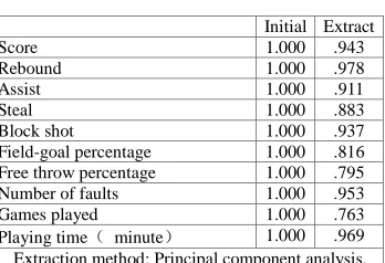
By Table 2 showed common factor variance, it is clear: each common factor that is extracted nearly is above 80%, therefore the extracted common factors explanatory ability on each variable is stronger. That means each indicator that is extracted has higher evaluation degree on player comprehensive ability.
Table 2: Common factor variance
Initial Extract
Score 1.000 .943
Rebound 1.000 .978 Assist 1.000 .911
Steal 1.000 .883
Block shot 1.000 .937 Field-goal percentage 1.000 .816 Free throw percentage 1.000 .795 Number of faults 1.000 .953 Games played 1.000 .763 Playing time( minute) 1.000 .969 Extraction method: Principal component analysis.
By following Table 3, it is clear that for output result, only the former three feature roots are above 1, the former three factors’ variance contribution rate is
89
.
481
%
, therefore it selects the former three factors is enough to describe players’ comprehensive ability level.Table 3: Explanatory total variance
Component Initial feature value Extract squares sum and input Rotate squares sum and input Total Variance % Accumulation % Total Variance % Accumulation % Total Variance % Accumulation % 1 6.419 64.186 64.186 6.419 64.186 64.186 4.171 41.705 41.705 2 1.362 13.620 77.806 1.362 13.620 77.806 3.177 31.768 73.474 3 1.167 11.675 89.481 1.167 11.675 89.481 1.601 16.007 89.481 4 .492 4.918 94.399
5 .328 3.283 97.682 6 .111 1.115 98.796 7 .089 .887 99.683 8 .015 .148 99.831 9 .011 .109 99.940 10 .006 .060 100.000
Extraction method: Principal component analysis.
[image:2.595.71.542.590.717.2]Figure 1: Scree plot
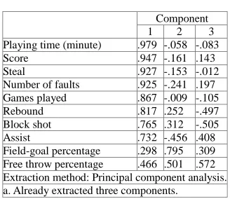
As following Table 4, it shows each factor to each player indicator variable impact.
Table 4: Component matrix
Component 1 2 3 Playing time (minute) .979 -.058 -.083 Score .947 -.161 .143 Steal .927 -.153 -.012 Number of faults .925 -.241 .197 Games played .867 -.009 -.105 Rebound .817 .252 -.497 Block shot .765 .312 -.505 Assist .732 -.456 .408 Field-goal percentage .298 .795 .309 Free throw percentage .466 .501 .572 Extraction method: Principal component analysis. a. Already extracted three components.
Player each indicator ability model is as following:
1
0.947
10.161
20.143
3 1ZX
=
F
−
F
+
F
+
ε
2 0.817 1 0.252 2 0.497 3 2
ZX = F + F − F +
ε
3
0.732
10.456
20.408
3 3ZX
=
F
−
F
+
F
+
ε
4
0.927
10.153
20.012
3 4ZX
=
F
−
F
−
F
+
ε
5
0.765
10.312
20.505
3 5ZX
=
F
+
F
−
F
+
ε
6 0.298 1 0.795 2 0.309 3 6
ZX = F+ F + F +
ε
7
0.466
10.501
20.572
3 7ZX
=
F
−
F
+
F
+
ε
8
0.925
10.241
20.197
3 8ZX
=
F
−
F
+
F
+
ε
9 0.867 1 0.009 2 0.105 3 9
ZX = F − F − F +
ε
10
0.979
10.058
20.083
3 10ZX
=
F
−
F
−
F
+
ε
Among them:
ZXi
represents thei
indicator individual ability contribution;F
irepresents thei
common factor;i
ε
represents thei
extrinsic factor.In expression, for each indicator variable after standardization,
ε
i represents special factor, is the other factoraffects the variable except for the three common factors. Originally, it designs ten indicators to show players’ comprehensive ability level, but after factor analysis, only needs three factors then can describe player comprehensive ability level influence status.
[image:3.595.224.388.265.407.2]Table 5: Rotational component matrix
Component 1 2 3
Assist .953 .011 .043
Number of faults .899 .351 .144
Score .852 .429 .182
Steal .769 .531 .098
Playing time( minute) .730 .644 .146 Games played .611 .607 .146
Rebound .278 .941 .122
Block shot .204 .934 .153 Field-goal percentage -.061 .213 .876 Free throw percentage .325 .033 .829 Extraction method: Principal component analysis.
Rotation method: Orthogonal rotation method with Kaiser standardization. a. Rotation makes convergences after five times iteration.
By Table 5, it is clear that the first common factor has larger loading in
X
1.、 3
X
、
X
4、 8X
、 9
X
、 10
X
, it mainly reflects player attack ability from score, assist, steal, fault, games played and playing time these aspects, which can
be named as attack factors. The second common factor has larger loading
X
2、 5
X
, it reflects player defense ability from rebound and block shot aspects, therefore named them as defense factors. The third common factor has
larger loading in
X
6、 7
X
, it shows as field-goal percentage and free throw percentage, therefore named them as stable factors. It roughly conforms to practical status, each common factor significance is relative reasonable.
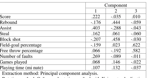
Factor score: Common factor score coefficient function cannot be got by factor load matrix through matrix transformation method, but only can be solved by adopted estimation method; the paper adopts regression method, express common factors into each variable linear form. Factor score coefficient matrix is as Table 6 show.
Table 6: Component score coefficient matrix
Component
1 2 3
Score .222 -.035 .010
Rebound -.176 .444 -.059
Assist .403 -.288 -.043
Steal .162 .061 -.060
Block shot -.207 .458 -.030 Field-goal percentage -.159 .023 .622 Free throw percentage .066 -.192 .582 Number of faults .269 -.089 -.011 Games played .068 .146 -.022 Playing time (mi nute) .107 .132 -.037 Extraction method: Principal component analysis.
Rotation method: Orthogonal rotation method with Kaiser standardization. Constitute the score.
It can directly write down each common factor score model:
1 1 2 3 4 5
6 7 8 9 10
0.222 0.176 0.403 0.162 0.207 0.159 0.066 0.266 0.068 0.107
F ZX ZX ZX ZX ZX
ZX ZX ZX ZX ZX
= − + + −
− + + + +
2 1 2 3 4 5
6 7 8 9 10
0.035 0.444 - 0.288 0.061 0.458 0.023 0.192 - 0.089 0.146 0.132
F ZX ZX ZX ZX ZX
ZX ZX ZX ZX ZX
= − + + +
+ − + +
3 1 2 3 4 5
6 7 8 9 10
0.010ZX -0.059ZX -0.043ZX 0.060ZX 0.030ZX 0.622ZX +0.582ZX 0.011ZX -0.022ZX 0.037ZX
F = − −
+ − −
SPSS has already put forward three common factors’ scores, saved them in fac_1~fac_3, according to each factor corresponding variance contribution rate as weights, calculate following comprehensive statistics:
λ
[image:4.595.185.431.414.544.2]=0.718F1+0.152F2+0.130F3
In SPSS, use program to calculate comprehensive factor score model:
Nets: Comp score=0.718* fac1_1 0.152* + fac2 _1 0.130* + fac3 _1
According to above principles, similarly, we can solve following seven teams’ comprehensive factors score model:
Mavericks:Comp score=0.625*fac1_2+0.255*fac2_2+0.120*fac3_2 Wizards:Comp score=0.705*fac1_3+0.177*fac2_3+0.118*fac3_3 Lakers:Comp score=0.710*fac1_4+0.173*fac2_4+0.117*fac3_4 Knicks:Comp score=0.651*fac1_5+0.231*fac2_5+0.118*fac3_5 Bobcats:Comp score=0.738*fac1_6+0.262*fac2_6
Hornets:Comp score=0.738*fac1_7+0.262*fac2_7
By above model, it can respectively calculate each team every player comprehensive score.
PLAYER ABILITY AND PLAYER OBTAINED SALARY RELATIONSHIP MODEL
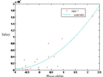
[image:5.595.229.396.362.487.2]By analysis, it is clear that player obtained salary high-low is closely related to player himself comprehensive ability, by analyzing mastered data, we establish salary and comprehensive ability regress model. Similarly, we take nets as an example, use MATLAB function to make quadratic fitting and get Figure 2.
Figure 2: Salary and comprehensive ability fitting curve
That:
2
( ) 1* 2 * 3
f x =p x +p x+p
Among them:
p1 = 1.499e+006 confidence interval is (2.044e+005, 2.794e+006) p2 = 3.201e+006 confidence interval is (1.361e+006, 5.041e+006) p3 = 2.026e+006 confidence interval is (8.46e+005, 3.207e+006)
R-square: 0.7829 Adjusted R-square: 0.7574
Table 7: Ten players’ actual salary and deserved salary
Player Player rank in list
Actual consulted salary
Deserved salary according to model calculation
Additional salary by calculating
Additional salary in rank
Calculation and actual additional parts differences Rashard Lewis 1 21136631 1458542.851 19678088.149 21167231 1489143 Kobe Bryant 2 25244493 9646284.171 15598208.829 19693258 4095049 Antawn Jamison 3 15076715 6257564.571 8819150.429 17402350 8583200 Amare Stoudemire 4 18217705 4231757.002 13985947.998 14918309 932361 Chris Karman 5 14030000 8313528.642 5716471.358 14613480 8897009 Corey Maggette 7 10262069 4546489.131 5715579.869 12862248 7146668 Dirk Nowitzki 8 19092873 4426000.000 14666873.000 12851295 -1815578 Deron Williams 9 16359805 12461790.076 3898014.924 12784867 8886852 Tyrus Thomas 10 7305785 1941601.922 5364183.078 12459225 7095042
Note: Play No.6 is not taken into consideration here because he is free player. In order to more clearly show the two relationships, we use EXCEL to draw, as following Figure 3.
Figure 3: Player actual salary and deserved salary curve graph
According to above Figure 3, we can clearly see that former ranking players’ actual salary and deserved salary gap is larger, while the two gaps gradually reduces with the later ones, which shows the overpaid gets more serious while ranks in the former.
CONCLUSION
The paper adopts factor analysis, better integrates player each ability variable, especially considers many effects impacting, selects nets data as center point, and gets verification by other teams. Finally it also takes errors analysis, result relative conforms to practice. But the shortcoming in the paper is that it only selects regular seasons, player’ rebound ability and some teams eliminate partial players.
REFERENCES
[1] CHEN Jian, YAO Song-ping. Journal of Shanghai Physical Education Institute, 2009, 33(5). [2] Wang Luning et al. China Sport Science, 1999, 19(3), 37-40.
[3] MAO Jie, SHAN Shuguang. Journal of Wuhan Institute of Physical Education, 2012, 46(2), 70-73, 87. [4] ZHANG Lei. China Sport Science and Technology, 2006, 42(1), 50-52.
[5] FU Fan-fei, YU Zhen-feng, ZHANG Quan-ning. Shandong Sports Science & Technology, 2006, 28(2), 24-25. [6] Wang Luning et al. China Sport Science, 1999, 19(3), 37-40.
[7] LI Ji-hui. Journal of Shenyang Sport University, 2006, 25(2), 63-66.
[8]YANG Yue-qing, RAO Han-fu, LEN Ji-lan. Journal of Hubei Sports Science, 2003, 22(2), 204-205. [9] Xiaomin Zhang. Journal of Chemical and Pharmaceutical Research, 2013, 5(12), 8-14.
[10] Wang Bo; Zhao Yulin. Journal of Chemical and Pharmaceutical Research, 2013, 5(12), 21-26. [11] Mingming Guo. Journal of Chemical and Pharmaceutical Research, 2013, 5(12), 64-69.
[image:6.595.186.426.241.351.2]