Forecasting CO2 emissions of power system in China using Grey Markov model

Journal of Chemical and Pharmaceutical Research, 2014, 6(7):387-393

Research Article

ISSN : 0975-7384

CODEN(USA) : JCPRC5

Forecasting CO

2

emissions of power system in China using

Grey-Markov model

Jie Xu

1,2

and Yuansheng Huang

1

1_{School of Economics and Management, North China Electric Power University, Beijing, China} 2_{College of Management, Hebei University, Baoding, China}

_____________________________________________________________________________________________

ABSTRACT

The greenhouse effect and its extension affecting is one of the key issues to governments and academics currently. Study shows, CO2 produced from burning fossil fuels are liable 2/3 of the above-mentioned problems. CO2

emissions in China are mainly concentrated in the power plants. In this paper, Gray - Markov method is used for long-term load forecasting, combined with the prediction of power generation coal consumption value. Meanwhile, the carbon emissions of power system in 2020-2050 are estimated through the prediction. The results show that: the power system 2020, 2030, 2040 and 2050 carbon emissions are：7.7254 billion tons, 20.0616 billion tons, 51.0740

billion tons and 131.3582 billion tons. Basis on that, we analyze the trend of power system low-carbon development. Then provide some suggestions to reduce CO2 emissions of power system from the level of the national policy, the

level of power generation components, power grid optimize and dispatching in the future.

Key words: Grey-Markov model, load forecasting, power system, CO2 emissions

_____________________________________________________________________________________________

INTRODUCTION

With the rapid development of the global economy, carbon dioxide produced by excessive burning of fossil fuels caused global warming and serious environmental problems. As a result, global warming had become the environmental problems that the entire human society has to face, and attracted great attention worldwide.

China has achieved rapid economic development, at the same time the carbon dioxide emissions increased. At present, China's carbon dioxide emissions ranked first in the world exceeding the United States. According to the data of China Energy Report (2008) Carbon Emissions Research, carbon dioxide emissions in China are mainly concentrated in the power plants, industry and transportation, these three sectors’ emissions are about 63-73% of total emissions. Power industry was one of the main sectors of carbon dioxide emissions in the national economy, its emissions are 38.76% of total emissions [1]. Therefore, the power industry has significant reduction space. Understanding the carbon emissions of power sector, and projecting its future development trend have great significance in lowering carbon dioxide emissions of the power industry.

______________________________________________________________________________

RESEARCH METHODOLOGY

For load forecasting, there is systematic research, current trend in power load forecasting technology is: extrapolation forecasting techniques, regression model forecasting techniques, time series forecasting techniques, gray prediction technology. Among them, the gray prediction technology is widely used in the short, medium and long term power load forecasting for small sample size, the higher the prediction accuracy [2]. On this basis, there is a lot of research of the application of improved gray prediction technology in load forecasting. This paper uses Grey - Markov model for load forecasting since Grey model needs small sample size but can give long term prediction. This paper uses gray rolling forecasting techniques, It uses GM (1,1) model to predict the next value, and then added them to the data at the same time removed the oldest value, keeping the number of columns constant. Then feed the data to the GM (1,1) model, repeating the process until the predetermined goal and prediction accuracy are reached. In the end, we combine with Markov techniques. Gray model and Markov chain can both be used for time series prediction, gray system changes the processing method for stochastic problems, it takes the randomness of the system as a gray, has application in systems when information is unknown or unclear. But Grey forecasting is generally used with less data, short time frame and little fluctuation, the predicted trend is a relatively smooth curve, monotonically decreasing or increasing. In the presence of random fluctuation, there will be predictions that are too high or too low. The Markov chain is the study of random variation system, an n-order Markov chain consists of a collection of n states

{ ,

a a

_{1 2}

,

⋅⋅⋅

,

a

_n

}

with a set of transition probability

P i j

_ij

( ,

=

1, 2,

⋅⋅⋅

, )

n

to determine. In this process, any time can only be in one status, if in the state

a

_i at time k, then at time k + 1 in the state

j

a

,transition probability

P

_ij reflect the influence degree of each factor, so the Markov chain is suitable for predicting dynamic process with large random fluctuations, and makes up for the weakness of the gray prediction. The two models complement each other and provide a practicality.

The establishment of gray model GM (1,1)

GM (1,1) model established the differential equation after generating process to the raw data. Establish GM (1,1) model requires only a few columns

X

(0): Let

(0) (0) (0) (0)

(

(1),

(2)

( ))

X

=

X

X

⋅⋅⋅

X

n

Take the series 1-AGO (Accumulated Generating Operation), so

(1) (1) (1) (1)

(1) (1) (0) (1) (0)

(

(1),

(2)

( ))

(1),

(1)

(2) ,

(

1)

( ))

X

X

X

X

n

X

X

X

X

n

X

n

=

⋅⋅⋅

=

+

⋅⋅⋅

− +

In the formula (1) (0) 1

( )

(

( ))

k

m

X

k

X

m

=

=

_∑

k

=

1, 2,

⋅⋅⋅

,

n

Generating the original series by the accumulation weakened the impact of bad data in original data, established the model after it became a regular sequence.

Using

X

(1) to constitute albino differential equations: (1)

(1)

dX

aX

u

dt

+

=

Solving Parameters

a u

,

using the least square method 1

[ , ]

T

(

T

)

T _N

X

=

a u

=

B B

−

B Y

(1) (1)

(1) (1)

(1) (1)

1

(1)

(2)

1

2

1

(2)

(3)

1

2

1

(

1)

( )

1

2

X

X

X

X

B

X

n

X

n

−

+

−

+

=

(0) (0) (0)

(2), (3), ( ) T

N

Y =_X X ⋅⋅⋅X n _

Get Gray model is: (1) (0)

(0) (1) (1)

(0)

ˆ

₍

₁₎

_[

₍₁₎

_]

_{, (}

_{(0,1, 2,}

₎

ˆ

₍

₁₎

ˆ

₍

₁₎

ˆ

_{( )}

(1

)[

(1)

]

, (

(0,1, 2,

)

ak

a ak

u

u

X

k

X

e

k

a

a

X

k

X

k

X

k

u

e

X

e

k

a

−

−

+ =

−

+

=

⋅⋅⋅

+ =

+ −

= −

−

=

⋅⋅⋅

The establishment of improved Gray-Markov model

The basic idea of Grey-Markov prediction model is: first establish the gray GM model, obtained the fitted curve; according to fitting curve can be divided into several dynamic range, and then through the Markov transition probability matrix predict the next state, calculate the predicted values. Specific steps are as follows:

The first step: In accordance with the aforementioned improved gray model GM (1.1), calculated predicted value (0)

ˆx

.

The second step: state divided

Let the original sequence is:

x

(0)

=

{

x

(0)

(1),

x

(0)

(2)

⋅⋅⋅

x

(0)

( )}

n

The analog values of original sequence is:

x

ˆ

(0)

=

{ (1), (2)

x

ˆ

x

ˆ

⋅⋅⋅

x n

ˆ

( )}

When the random sequence

x

(0) meet the characteristics of Markov chain, divided (m +1) parallel curve to the variation curve

x k

ˆ( )

into m states

F F

₁

,

₂

,

⋅⋅⋅

F

_m, where the value of m based on the original sequence and research object .

Firstly, forecasts for each thermal generating capacity using gray prediction model, obtains prediction residuals with actual and predicted value. Divides residual state as follows according to the proportion of the actual value, in this paper makes the load forecasting results as follows:

(1) The residual proportion is down to -4%, which means that the value of power load forecasting has been seriously underestimated, called a state F1;

(2) The residual proportion is in (-4%, 0], which means that the value of power load forecasting was normal underestimated, called a state F2;

(3) The residual proportion is in (0, 4%], which means that the value of power load forecasting is normal overestimated, called a state F3;

(4) The residual proportion is up to 4%, which means that the value of load forecasting was seriously overestimated, called a state F4.

The third step: determined the state transition probability matrix

If

M

_i is the initial sequence of samples in the state

F

_i,

M

_ij

( )

m

is the initial data sample that

F

_i through the m-step transition to

F

_j, _ij

( )

ij

( )

(

1, 2,

)

i

M m

p m

i

n

M

=

=

L

is called the state transition probability.

So the state transition probability matrix is:

( ) ( ) ( )

11 12 1

( ) ( ) ( )

( ) 21 22 1

( ) ( ) ( )

m m m

n

m m m

m n

m m m

p

p

p

p

p

p

p

p

p

p













=

_

_













L

L

L

L

L

L

______________________________________________________________________________

The fourth step: forecasting

According to Markov prediction model

s

₁

=

s

₀

* ;

P s

₂

=

s

₀

*

P

2

;

L

;

s

_n

=

s

₀

*

P

n can be predicted.

[image:4.595.76.547.152.303.2]

DATA SOURCES

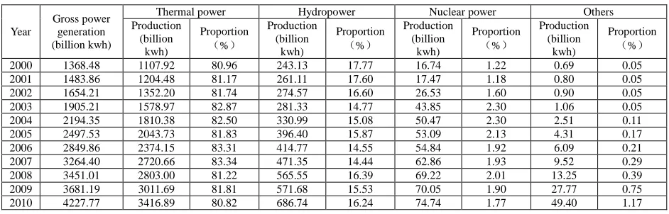
Table 1: 2000-2010 China's power structure and composition

Year

Gross power generation (billion kwh)

Thermal power Hydropower Nuclear power Others Production

(billion kwh)

Proportion

（%）

Production (billion

kwh)

Proportion

（%）

Production (billion

kwh)

Proportion

（%）

Production (billion

kwh)

Proportion

（%）

2000 1368.48 1107.92 80.96 243.13 17.77 16.74 1.22 0.69 0.05 2001 1483.86 1204.48 81.17 261.11 17.60 17.47 1.18 0.80 0.05 2002 1654.21 1352.20 81.74 274.57 16.60 26.53 1.60 0.90 0.05 2003 1905.21 1578.97 82.87 281.33 14.77 43.85 2.30 1.06 0.05 2004 2194.35 1810.38 82.50 330.99 15.08 50.47 2.30 2.51 0.11 2005 2497.53 2043.73 81.83 396.40 15.87 53.09 2.13 4.31 0.17 2006 2849.86 2374.15 83.31 414.77 14.55 54.84 1.92 6.09 0.21 2007 3264.40 2720.66 83.34 471.35 14.44 62.86 1.93 9.52 0.29 2008 3451.01 2803.00 81.22 565.55 16.39 69.22 2.01 13.25 0.39 2009 3681.19 3011.69 81.81 571.68 15.53 70.05 1.90 27.77 0.75 2010 4227.77 3416.89 80.82 686.74 16.24 74.74 1.77 49.40 1.17

Table 1 shows China's power structure, thermal power generation was more than 80% of the total generating capacity, and the generating capacity increased year by year; hydropower generating capacity maintains constant proportion of total generating capacity at 14.44-17.77%, and nuclear power generation has been very small proportion of the total generating capacity, the highest being 2.30% in year 2003 and 2004, others such as wind power, etc. is minimal. Hydropower has almost zero carbon emissions, nuclear chain greenhouse gas emissions is equivalent to 13.71g CO2 (kwh) -1, while the coal chain greenhouse gas emissions is equivalent to 1302 g CO2 (kwh) -1 _{[3]. Thermal power is basically dominated by coal generation, meantime, the generators tend to have a longer} service life, which implies that China's power industry has a strong carbon lock-in effect, that is the power industry CO2 emissions will be "locked" by the current power structure in the future for a long period of time [4,5]. That is, the power system of carbon emissions will be mainly from thermal power generation. So in this paper, load forecast of power system for the next few years based on coal power load data for each year, and then carbon emissions of power system can be calculated according to the coal consumption.

RESULTS AND DISCUSSION

Bases on the data of the power load in 2000-2010, according to the above method predicted power load for several years in the future. Taking into account the power system of carbon emissions mainly from thermal power, in this paper, we select the thermal power data.

Thermal power predictive value using Grey-Markov method

According to the aforementioned gray model GM (1,1), take the Thermal power data in 2000-2010 as the original sequence for grey prediction, forecast values as follows:

Table 2: Thermal power predictive value Year Generating capacity

(billion kwh) Year

[image:5.595.96.521.81.237.2]

Fig.1: Original data compared with predicted values in 2000-2010 According to the aforementioned method, divide the status of forecasting values in 2000-2010

Table 3: Divide the status of gray forecasting values Year Actual value

(billion kwh)

Forecasting value

(billion kwh) Residuals

Residuals

proportion (%) Status 2000 1107.92 1107.92 0 0 2 2001 1204.48 1304.44 -99.96 -8.30 1 2002 1352.20 145511 -102.91 -7.61 1 2003 1578.97 1623.18 -44.21 -2.80 2 2004 1810.38 1810.67 -0.29 -0.02 2 2005 2043.73 2019.81 23.92 1.17 3 2006 2374.15 2253.10 121.05 5.10 4 2007 2720.56 2513.35 207.21 7.62 4 2008 2803.00 2803.65 -0.65 -0.02 2 2009 3011.69 3127.48 115.79 -3.84 2 2010 3416.89 3488.72 -71.83 -2.10 2

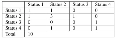
The frequency statistics of the status transition from residuals can be obtained by Table 4: Table 4 Frequency statistics of the residuals status transition

Status 1 Status 2 Status 3 Status 4 Status 1 1 1 0 0 Status 2 1 3 1 0 Status 3 0 0 0 1 Status 4 0 1 0 1 Total 10

Determine the state transition probability matrix

State transition probability matrix from the residuals frequency statistics for status transition is:

0.5 0.5 0 0

0.2 0.6 0.2 0

0 0 0 1

0 0.5 0 0.5

P

 

 

 

=_{ }

 

 

According to Markov prediction model,

s

₁

=

s

₀

* ;

P s

₂

=

s

₀

*

P

2

;

_L

;

s

_n

=

s

₀

*

P

n, It can be obtained the state transition forecasting value of 2020, 2030, 2040, 2050.

S0= (0.182 0.545 0.091 0.182)

Final predictive value is:

V

′ =

V

(1

+ ×

P M

)

0 500 1000 1500 2000 2500 3000 3500 4000

2000 2001 2002 2003 2004 2005 2006 2007 2008 2009 2010 time

g

e

n

e

ra

tin

g

c

a

p

c

a

ity

(b

ill

io

n

k

w

h

)

[image:5.595.212.398.486.548.2]

______________________________________________________________________________

In the formula,

V

′

is the final predictive value,

V

is the gray predictive value,

P

is the largest probability value of the annual status,

M

is the median,

M

=

0.5 (

×

U

+

L

)

, U is the upper limit of the status,

L

is the lower limit of the status. Among them, the states 1 and 4 take directly -2% and 2%. So it can be obtained the load forecasting values: 2020 is 10504.67 billion kwh, 2030 is 31372.60 billion kwh, 2040 is 93620.31 billion kwh, 2050 is 279556.99 billion kwh.

Coal consumption values forecast

Most coal-power chain carbon emissions come from power generation. The major factor that impacts carbon emissions of power plants is coal consumption level. Its level is directly related not only to carbon emissions of the power plant，but also the coal-power chain carbon emissions. In recent years, a large number of old and small

[image:6.595.187.429.269.369.2]

thermal powers were eliminated in China. Therefore, coal-fired power plants had a certain decline in coal consumption. the specific data are showed in table below. However, compared with developed countries China's has a long way to go until the problem of coal consumption is solved. But coal consumption trends and technological innovations in China show that coal consumption of China can be greatly declined in the future.

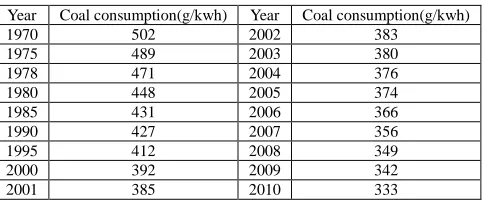
Table 5 Coal consumption data 1970-2010

Year Coal consumption(g/kwh) Year Coal consumption(g/kwh) 1970 502 2002 383

1975 489 2003 380 1978 471 2004 376 1980 448 2005 374 1985 431 2006 366 1990 427 2007 356 1995 412 2008 349 2000 392 2009 342 2001 385 2010 333

Based on the above data, using the improved GM (1.1), that is gray rolling forecast, prediction results can be obtained as follows: 2020 is 293.822g/kwh, 2030 is 253.068g/kwh, 2040 is 217.968g/kwh, 2050 is 187.736g/kwh. Calculation of power system carbon emissions

When power plant is in operation, It produced greenhouse gases mainly CO2 and a small amount of N2O. NOx is generated by conventional combustion mode in coal-fired power plants, NO accounted for about 90%, N2O accounts for only about 1% [6]. According to the recommended values by National Development and Reform Commission Energy Research Institute and the Energy Handbook 2006, One ton of standard coal’s CO2 emission coefficient (t / tce) is 2.4567tCO2/tce, One ton of standard coal’s NOx emission coefficient (t / tce) is 0.0156tNOx/tce. In addition, according to the greenhouse gases GWP default given by IPCC Third Assessment Report (2001), CO2 is 1gCO2 equivalent / g greenhouse gases, N2O is 296 gCO2 equivalent / g greenhouse gases. Carbon emissions each year can be obtained by calculating. The result is: the CO2 emission of 2020 is 7.7254 billion tons, 2030 is 20.0616 billion tons, 2040 is 51.0740 billion tons, 2050 is 131.3582 billion tons.

According to China's power industry development characteristics and the characteristics of primary energy, the most effective measures of CO2 emission reduction is to adjust the industrial structure. That is, orderly and vigorously develop hydropower, wind and solar clean energy generation under the premise of protection of environment. Substituting hydropower, wind power and solar power for thermal power can bring a decrease of CO2 emissions about 1kg per kwh, thus low-carbon benefits are obvious. Developing such energy plays an important role in achieving the development of low-carbon electricity in China. According to our calculations, for example, if the proportion of thermal power generation of total generated energy decrease by 20% in 2050, the CO2 emissions would be reduced by about 26 billion tons. However, clean energy also has a series of problems to be solved, including higher cost and higher demands of corresponding supporting of electricity grid and cost requirements. Development of large-scale clean energy power will cause a large increase of cost burden to power plants.

Combined Cycle (IGCC) power generation technology. These techniques really applied to power generation need some time and effort.

CONCLUSION

The results showed that: CO2 emissions from the power system have a rising trend. If the existing power structure is kept, emission reduction works of power systems will have a long way to go. To construct of low-carbon electricity system, not only the existing fossil fuel generators need to reduce emissions, but also renewable energy and other clean energy will be relied on in the long term. So we can work from the following aspects.

On the level of the national policy, we can levy "carbon tax" timely and at appropriate which tax will be able to be internalize the external costs of the greenhouse gas emissions directly and effectively. It will be of great benefit to settle the long-term environmental problems. We can also establish and improve the carbon market. Carbon trading market will change with prices and supply-demand changes in the overall operation, but there are many issues in the implementation of the carbon trading market that need further study. Government departments need to establish the industry's carbon emissions targets and strictly supervise execution, Implement differential pricing to different power plants to encourage the implementation of low-carbon electricity, and also introduce some incentive measures to promote energy conservation and emission reduction to small and medium enterprises.

On the level of power generation components encourage the low-carbon development of power generation enterprises, increase low-carbon technology innovation and application of fossil fuel in power generation, the development of recycling economy; adjust carbon structure appropriate, develop renewable energy vigorously, increase nuclear power and hydropower proportion appropriate.

On the level of the power grid optimize the layout of power plants and power grid, increase the smart power grid construction; strengthen low-carbon electricity scheduling constraints; continue to build UHA substation and digital substation.

Acknowledgments

The authors wish to thank the Project supported by the key project of central university research in Education Ministry, China. (ID. 12ZX21)

REFERENCES

[1]Yiming Wei, Lancui Liu,Ying Fan, et al. China Energy Report (2008): CO2 Emissions Research, Science Press. Beijing, 2008.

[2]Julong Deng. Grey Prediction and Decision. Huazhong University Press. Wuhan, 1986.

[3]Zhonghai Ma; Ziqiang Pan; Huimin He. Chinese Journal of Nuclear Science and Engineering., 1999,19(3),268. [4]Kunmin Zhang, Jiahua Pan, Dapeng Cui. Introduction of Low Carbon Economy, China Environmental Science Press, Beijing, 2008.

[5]Grubb M, Jamasb T, Pollitt M. Delivering a Low-carbon Electricity System, Cambridge University Press, UK,

2008.

[6]Chong-qing KANG; Tian-rui ZHOU; Qi-xin CHEN; Jun GE. Power System Technology., 2009,17,1-6. [7]Zewen Wang; Wen Zhang; Shufang Qiu. Mathematics in Practice and Theory., 2009, 39(1), 125-131.

[8]Min Li ; Hui Jiang ; Yin-hua Huang ; Xiaoming Song. Proceedings of the CSU-EPSA., 2011, 23(2), 131-134. [9]Hui-ming Xia; Zhi-gang Wang; Jin-lin Wu. Science Technology and Engineering., 2012, 23(12), 5884-5887. [10]Hsiao-Tien Pao; Hsin-Chia Fu; Cheng-Lung Tseng. Energy., 2012, 40(1), 400–409.