Difference limen for the Q factor of room modes

Difference limen for the Q­factor of room 

modes

Fazenda, BM, Avis, MR and Davies, W

Title

Difference limen for the Q­factor of room modes

Authors

Fazenda, BM, Avis, MR and Davies, W

Type

Conference or Workshop Item

URL

This version is available at: http://usir.salford.ac.uk/9452/

Published Date

2003

USIR is a digital collection of the research output of the University of Salford. Where copyright 

permits, full text material held in the repository is made freely available online and can be read, 

downloaded and copied for non­commercial private study or research purposes. Please check the 

manuscript for any further copyright restrictions.

Audio Engineering Society

Convention Paper

Presented at the 115th Convention

2003 October 10–13

New York, New York

This convention paper has been reproduced from the author's advance manuscript, without editing, corrections, or consideration by the Review Board. The AES takes no responsibility for the contents. Additional papers may be obtained by sending request and remittance to Audio Engineering Society, 60 East 42nd Street, New York, New York 10165-2520, USA; also see www.aes.org. All rights reserved. Reproduction of this paper, or any portion thereof, is not permitted without direct permission from the

Journal of the Audio Engineering Society.

___________________________________

Difference Limen for the Q-factor of Room

Modes

B.M.Fazenda1_{, M.R.Avis}1_{, and W.J.Davies}1

1The University of Salford, Salford, Manchester, M5 4WT, UK

[email protected]; [email protected]; [email protected]

ABSTRACT

A subjective test study was carried out in order to identify the perceptibility of changes in the Q-factor of room modes. The experimental technique concentrates on the identification of difference limen for three levels of Q-factor referring to modes in rooms used for critical listening. Trends show that changes in higher Q values are more perceptible than those for lower Q values. The results may be applied in decisions for treatment of modes in common listening and control rooms.

1. INTRODUCTION

It is well known that one of the main problems in critical listening rooms is the effect of resonant modes, directly associated with the physical dimensions of the rooms [1,2,3,4,5]. Much work has been done in trying to avoid degenerate modes by defining optimum room ratios [4,6,7,8]. These techniques concentrate on optimising the room’s modal distribution at low frequencies, in an attempt to avoid either an amplification or attenuation of sound over certain frequency ranges. This issue is one that is highly dependant on source and receiver position as well as on room dimensions and also on the acoustic impedance at the boundaries of the space.

Complementary approaches have been to introduce acoustic absorption in order to ameliorate the response in the room at problematic frequency ranges. These solutions take the form of either passive absorption [10,11] or active absorption [12,13,14]. Both these approaches rely on altering the Q-factor of the modes removing some of the energy associated with them.

Fazenda, Avis and Davies

Difference Limen for Q-factor of room modes

There are various definitions for this frequency and for the same volume, different definitions lead to different cross over frequencies [7,15,16]. The definition for the Schroeder Frequency is associated with subjective perception of sound. It is defined as the frequency above which there are at least three resonances that overlap within their half power points (bandwidth). The study carried out by Bonello [9] uses the auditory critical bandwidth to define an optimum number of modes per frequency bandwidth.

Some work has been done specifically on subjective perception of low frequencies. The work of Olive, Schuck et al [17] looks at the subjective detection thresholds of single resonances at different low frequency centre frequencies and different levels of Q. From this work, results indicate that the Q of modes is an important factor in the detection of isolated resonances.

Current practice in industry regarding the design of critical listening spaces at low frequency is to decide on a room aspect ratio in order to avoid degenerate modes. However, in some cases, the designer is still faced with strong low frequency resonances when sound is generated in the room. The usual method to solve this problem is to use resonant absorbers which are optimally tuned at problematic frequencies. These devices remove some of the energy of resonant modes by altering their Q-factor or bandwidth.

In this paper, we set out to define a difference limen

(DL) for modal Q-factor in order to inform the use of various absorption techniques for the control of

low-frequency room modes. The subjective efficacy of a

given absorption treatment may then be evaluated,

from a set of known objective absorption

characteristics. This will lead to a more efficient use of absorption treatments, reflected in economy of materials, and to the specification of suitable sound field targets for novel control regimes [12,13,14].

The hypothesis to be tested is that changes in the Q-factor of room modes are perceptible and alter the perception of sound in the room. The present experiment tests this hypothesis and aims to identify the difference limen for these changes. This study is novel in the fact that it investigates the effects of room modes as perceived in a room environment for reproduced music signals, as opposed to isolated resonances assessed using noise or impulsive signals. The study of effects on a wider number of modes leads to a more generalised understanding of the behaviour of absorption with wider applications in the current practices for room acoustics.

2. BINAURAL MODEL OF A LISTENING SPACE

One of the major problems on subjective testing for room acoustics has been the difficulty in changing acoustic parameters rapidly [19]. The removal and introduction of large items to control the acoustic sound field is invariably time consuming. Altering the acoustic characteristics whilst maintaining the waiting time between auditions to a minimum has always been a crucial requirement given the relative short acoustic “memory” of subjects [20]. The experiment presented here explores the use of binaural reproduction over headphones to overcome this problem. It uses a virtual representation of a real room. This is created by the use of binaural recording techniques associated with an analytical model of the room at low frequencies. This approach enables the presentation of different low frequency acoustic conditions in sequence, without changing the high frequencies.

The generation of the audition samples is therefore divided into two main parts associated with a division of the audible frequency spectrum. These will be

referred to as Low and High frequency regions.

2.1. High Frequency Binaural Impulse Responses

It was decided to maintain a fixed and pre-determined high-frequency auralisation within the samples for audition, whilst manipulating their low-frequency characteristics. A dummy head was used to measure binaural room responses, which were used as the starting point for the design of the room auralisation on which the subjective test was based. The high frequency content of the audition samples contains spatial and temporal information which is crucial to the sensation of listening in a real room, and this data was obtained directly from the measured binaural impulse responses.

Two high-frequency reverberation conditions were tested. One binaural impulse response corresponds to a very low reverberation time (0.2 secs), associated with some types of professional control rooms [21]. Another binaural impulse response was measured with a longer reverberation time (0.5 Secs), more closely related to a listening room environment [22]. These reverberation values are an average taken from measurements in the 250 Hz to 8KHz bandwidth. The choice of two reverberation conditions was made in order to evaluate the masking effect of high frequency reverberation on the low-frequency difference limen of modal Q-factors.

AES 115TH CONVENTION, NEW YORK, NEW YORK, 2003 OCTOBER 10-13

2.2. Low Frequency Model

At this stage the low frequency modal behaviour of the measured room is still present in the original BIRs. This part of the response is removed using a Butterworth first order high-pass filter with a crossover frequency determined by the Schroeder Frequency.

After the filtering process it is then necessary to re-create the low frequency part of the room model. This is done by using biquad filters designed to match the centre frequencies of the modes in the room. The bandwidth of these filters is easily variable and will constitute the variable under subjective test.

Each modal resonance in the room may therefore be generated by a z-plane biquad. In this case, the response obtained is that of a band pass filter, where the centre frequency and bandwidth are dependant on pole angle and pole radius respectively.

In order to reconstruct a series of modes at different frequencies, several biquads can be cascaded. The case of the “pressure zone” in frequency or the “zeroth” mode can be modelled by designing a low pass filter using a real pole at 0° angle. The output gain of the filter section may be scaled by a multiplication factor in the difference equation.

Follows a list of the difference equations for the various types of filters used in the modelling of the low frequency region.

“Zeroth” mode -

(1)

( ) ( ) (

k

=

x

k

+

x

k

−

1

)

+

R

y

(

k

−

1

)

y

Single Mode –

( )

(

)

(

2

)

( )

(

2

)

...

...

1

2

2

−

+

−

−

+

−

=

k

Kx

k

Kx

k

y

R

k

y

Cos

R

k

y

p

p

θ

(2)

Where Rp is the pole radius, θ is the pole angle and K

is the output scaling factor. The filter coefficients can then be determined accordingly.

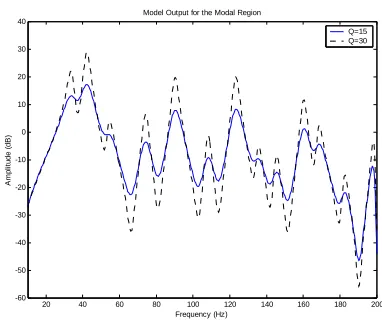
Figure 1 shows two different conditions at the model output, one with a high Q-factor, and one with a medium Q-factor.

20 40 60 80 100 120 140 160 180 200

-60 -50 -40 -30 -20 -10 0 10 20 30 40

Frequency (Hz) Model Output for the Modal Region

A

m

pl

it

ud

e (

d

B

)

Q=15 Q=30

Figure 1 – Frequency response for two cases of the modal response

The audition pairs are presented via headphones in a quiet, but not necessarily isolated or controlled environment. The headphones selected provide adequate levels of sound reduction from external noise and are capable of reproducing frequencies down to 30 Hz.

A batch of test samples ranging from minimum to maximum values of Q-factor were created previous to the running of the tests. This was done using a computer model where each sample was written into a .wav file. An automated test procedure accesses these files and plays A/B comparison pairs.

3. FORMING A MODEL ROOM

Fazenda, Avis and Davies

Difference Limen for Q-factor of room modes

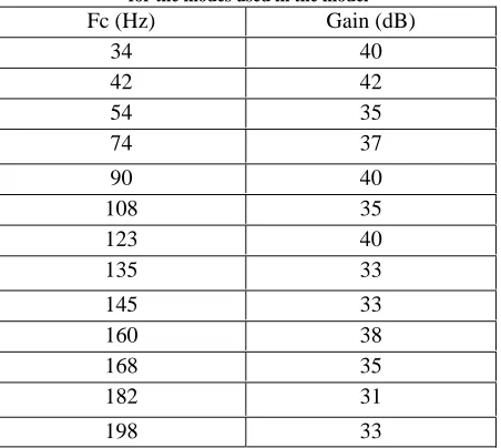
Table 1 – Centre frequencies and corresponding amplitudes for the modes used in the model

Fc (Hz) Gain (dB)

34 40 42 42 54 35 74 37

90 40 108 35 123 40 135 33 145 33 160 38 168 35 182 31 198 33

The Schroeder Frequency for the room was fs=212Hz, rounded to 200Hz for the transition frequency in the model. The mean modal Q-factor

measured in the room was Q(µ,δ)=(17+/-6.2).

It follows that in order to obtain valid results from any subjective experimental technique, only certain parameters should be allowed to vary whilst parameters which are not under study should be fixed. For this experiment, only the modal Q-factor was varied. The assumptions this implies are described below.

At any single position for a fixed size room any changes in the modal behaviour can only be associated with changes in the damping characteristics at the boundaries of the room.

As described previously, current practice on passive modal control takes the form of resonant absorbers. Most commonly these devices usually imply absorption over a wide bandwidth in order to effectively control a region of the frequency response rather than act on single modes. Hence, some of the assumptions for the present subjective experiment rely on the fact that changes in absorption characteristics at the boundaries of the space will affect the Q-factor of all modes simultaneously and to the same degree. Furthermore, in order to maintain modal Q-factor as the only variable being tested, the bandwidth of all modes below the Schroeder Frequency is assumed to be the same. In real applications this means that absorption increases proportionally to frequency and therefore higher order modes are more susceptible to the increasing

effects of absorption in the room. Hence, an experimental variation of modal Q value corresponds to altering the bandwidth of all modes by the same relative amount.

Another factor to take into account in forming the room model is the amplitude of each mode. In the experimental room model, changes are applied to the Q-factor as the single variable under test, given that amplitude and modal Q-factor are interdependent. The model, defines modal amplitudes which correspond to the ones measured in the “real” room (Table 1). These are then affected by the changes applied to Q-factor. As the Q’s of the modes change, this has an overall effect on their amplitudes (i.e. if the Q-factor of a mode decreases so does its amplitude). A single change in level with no associated change in Q-factor would indicate a movement of the listener in the room rather than a change to the boundary conditions, and this has been avoided.

Finally, because changes in the low frequency region of the samples affect their perceived loudness level, and because this is an important and extraneous psychoacoustic cue, all samples have been normalised to the same A weighted level.

4. THE TEST METHOD

The method used for the subjective experiments is similar to a 2 interval forced choice [18]. The subject listens to two music samples sequentially and is asked to state if there is any difference between them. The samples in each audition are referred to as

reference and modified. The reference sample represents a fixed condition against which the modified sample is compared. Subjects were asked to concentrate on the sound at the lower end of the spectrum – the bass.

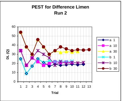
The process for identifying the difference limen for changes in Q of the modes is of an adaptive type. The amount of change applied to the modified sample is decided in such a way as to achieve the response in the least number of comparisons (auditions). The PEST (Parameter Estimation by Sequential Testing) convergence procedure achieves this by applying a series of decisions that are dependant on previous answers [18]. Figure 2 shows an example of the PEST answers for one of the subjects. The important point on the graph is the convergence of the answers towards what will be the difference limen for each case.

AES 115TH CONVENTION, NEW YORK, NEW YORK, 2003 OCTOBER 10-13

PEST for Difference Limen Run 2

20 30 40 50 60

1 2 3 4 5 6 7 8 9 10 11 12 13

Trial

DL

(Q

)

0 10

a 1 a 10 a 30 b 1 b 10 b 30

Figure 2 – PEST convergence results for one subject; a) Low RT, b) High RT

The test variables are as follows:

Each subject was tested for two high-frequency (above Schroeder) RT conditions (short - 0.2 secs, medium - 0.5secs), at 3 different reference Q values, low (Q=1), medium (Q=10) and high (Q=30) each.

Samples are presented through headphones at a level of 78.1 dB(A) SPL, calibrated at the microphones of the B&K Head And Torso Simulator (dummy head) and using a B&K 2231 sound level meter. The audition level is dependent on computer soundcard level output and was chosen to be close to 80 dB(A), which represents a comfortable and usual listening level in professional situations.

5. RESULTS AND DISCUSSION

An analysis of variance (ANOVA) was carried out in order to identify the significance and validity of experimental results. The factors involved are the Reverberation Time and three levels of reference

Q-factor. The levels for each factor are described as RT

Low, RT Med, Qlow, Qmed and Qhigh. One other factor that will be analysed is the effect of repeats for each subject.

Each subject tested for the above six cases and this was repeated three times. For the analysis these

repetitions are called RUN and this will become

another factor. The first analysis concentrates on the effect of RUN on the overall results. The significance for this factor is indicated in Table 2. In this case the result is above the statistical significance criteria p<0.05. This indicates that statistically there is no significant effect of the factor RUN on the results for the other two factors, RT and Q. In practice this result

shows that subjects were consistent across their 3 repeats. It also indicates that further analysis may be performed either on the whole set of data or just on

any single Run. The authors have chosen to include

the whole set of data for further analysis as this will lead to better statistical estimates.

Table 2 – ANOVA including three factors; RUN, RT and Q

Tests of Within-Subjects Effects Source Type III Sum of

Squares

df Mean Square

F Sig. (p)

RUNSphericity Assumed

60.03 2 30.01 1.41 0.270

RT Sphericity Assumed

168.68 1 168.68 11.43 0.008

Q Sphericity Assumed

2606.00 2 1303.00 65.99 0.000

However, and before concentrating on the final data there is an interesting fact that arises from analysing

each Run independently.

Table 3 shows the ANOVA performed on each Run

independently. The value of p indicates the

significance of each factor.

Table 3 – ANOVA results performed on each of the three runs individually

Tests of Within-Subjects Effects(a) Source

Type III Sum of Squares

df Mean Squar e

F

Sig. (p)

RUN1RT

Greenhouse-Geisser 42.50 1 42.50 2.45 0.152

Q

Greenhouse-Geisser 736.14 1.16 633.57 21.59 0.001

RUN2RT

Greenhouse-Geisser 24.70 1 24.70 0.87 0.377

Q

Sphericity

Assumed 803.09 2 401.55 32.73 0.000

RUN3RT

Greenhouse-Geisser 121.13 1 121.13 15.49 0.003

Q

Sphericity

Assumed 1133.88 2 566.94 33.48 0.000

(a) for different runs

The value for p associated with the factor RT is above

the usual criterion (p<0.05) for the first two Runs and

highly significant for the last Run (p<0.01). This is

an important result as it indicates that as subjects become more trained, they are better at distinguishing

different RT cases. In the context of studio control

Fazenda, Avis and Davies

Difference Limen for Q-factor of room modes

trained listener and therefore sensitive to the effects of reverberation time on the perception of low frequencies.

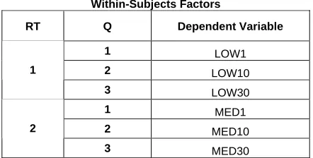
A new ANOVA was carried out using the whole set of data available. There were a total of 10 subjects resulting in 30 sample results for each factor.

Table 4 shows the arrangement of these factors for the analysis.Table 4 – Factors for the full ANOVA

Within-Subjects Factors

RT Q Dependent Variable

1 _LOW1

2 _LOW10

1

3 _LOW30

1 _MED1

2 _MED10

2

3 _MED30

Table 5 shows the results for the full ANOVA. Inspection reveals that RT is highly significant

(p<0.01), which indicates a significant effect of RT

on the results for DL of modal Q-factor. This leads to a definition of a different DL for the two RT cases tested. Further interpretation of results indicates high

significance for the experimental factor Q (p<0.001).

There are no significant interaction effects between the Reverberation Time of the samples and the level of reference Q on the difference limen registered. This means that the effect of reference Q on the determination of a difference limen was the same for both RT cases. In practice this indicates that varying RT has the same effect on the difference limen results, regardless of the reference Q-factor under test.

Table 5 – ANOVA for the full data

Tests of Within-Subjects Effects Source

Type III Sum of Squares

df Mean

Square F Sig. (p)

RT Greenhouse-Geisser 168.68 1.00 168.68 9.72 0.004

Error RT

Greenhouse-Geisser _{503.43 29.00 17.36}

Q Greenhouse-Geisser 2606.00 1.46 1789.85 84.01 0.000

Error Q

Greenhouse-Geisser _{899.60 42.22 21.31}

RT*Q Greenhouse-Geisser 22.14 1.23 18.04 0.61 0.470

Error RT*Q

Greenhouse-Geisser _{1045.71 35.59 29.38}

Table 6 below shows the mean Difference Limen for modal Q, in each of the cases tested.

Table 6 – Difference Limen for Q-factor in room modes

Descriptive Statistics

Mean Std.

Deviation N

LOW1 15.2 6.3 30

LOW10 _{10.1 5.0 30}

LOW30 6.8 4.6 30

MED1 _{18.1 3.9 30}

MED10 _{11.9 4.3 30}

MED30 8.0 4.4 30

It is clear that the difference limen increases with decreasing Q-factor. Additionally, the values for the difference limen at medium RT are higher than those for the low RT case.

In practical terms these results indicate that subjects were able to detect a smaller change in the parameter Q-factor at higher levels of Q. For room applications this indicates that as the desired level of Q decreases, the amount of change necessary to obtain a perceptible difference needs to become larger.

In the case of the reverberation time these results indicate that it is more difficult to perceive a difference at higher RT levels. Hence, in room applications it may be important to have some high frequency energy that will to some extent “mask” the effects of low frequency resonances. On the other hand, in order to produce a perceptible difference at low frequencies, the effective change on the Q-factor of the room modes needs to be larger in rooms with a higher mid-frequency reverberation time.

The average results may be presented individually for each of the reverberation time conditions. This is shown in Table 7.

Table 7 – Mean values for Q-factor difference limen at two RT cases

95% Confidence Interval RT

Mean Std. Error

Lower Bound Upper Bound

1 _{10.7 0.7 9.2 12.2}

2 12.6 0.5 11.6 13.7

AES 115TH CONVENTION, NEW YORK, NEW YORK, 2003 OCTOBER 10-13

Statistically, the difference between the two RT cases has been proven significant (Table 5). However, the result above shows a difference of approximately 2 in Q-factor. This is in practice a very small difference and indeed much smaller that any of the DL presented on table 6. It seems reasonable to assume that for the generalization of a difference limen for the Q-factor in room modes, the effect of reverberation time may be disregarded.

Table 8 shows the mean values calculated for the different levels of reference Q across the two RT cases.

Table 8 – Mean values for Q-factor difference limen at three reference Q

cases

Q Lower

Bound

Upper Bound

1 16.6 0.8 15.0 18.3

2 11.0 0.6 9.8 12.2

3 7.4 0.6 6.1 8.7

Mean Std. Error

95% Confidence Interval

Furthermore, statistical analysis shows that there is a highly significant probability that the difference limen for Q-factor follows a linear trend (table 9). This result originates from the ANOVA analysis on the raw data.

Table 9 – Within Subjects Contrasts – Linear Trends

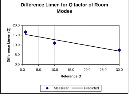
Following up on this statistical significant result, a prediction of the expected difference limen may be generalised across a range of Q-factors. This may be done by calculating the line of best fit in the available data. Figure 2 shows the experimental results calculated for the DL (from table 8) and a regression analysis that produces a best-fit line.

Difference Limen for Q factor of Room Modes

0.0 5.0 10.0 15.0 20.0

0.0 5.0 10.0 15.0 20.0 25.0 30.0

Reference Q

D

iffe

re

nc

e

Lim

e

n (Q)

Measured Predicted

Figure 3 – Data representing a generic difference limen for the Q-factor of room modes; Experimental contrasted with a

regression analysis prediction

Given the small number of data points, this extrapolation is clearly indicative rather than conclusive. More data points would, of course, be required to provide a better confidence on the linear relationship between Q-factor and difference limen.

Figure 3 shows an intercept in the region Q=16. This suggests that using this data set, a modal Q of at least 16 is required to detect the presence of a resonance, and that modes with lower Q will not be detected (since they will not be differentiable from the case where Q=0 – no resonance). Q=16 is therefore the threshold value below which any further room treatment would be unnecessary.

Source RT Q

Type III Sum of Squares

df Mean

Square F Sig. Linear 2562.25 1 2562.25 120.29 0

Quadratic 43.75 1 43.75 4.501 0.043

Q Earlier work by Olive et al suggests that modal

audibility in the steady state is inversely proportional

to modal Q, but using square pulses (width=10ms)

the detection threshold and Q-factor are directly

proportional. Even though this paper refers to an experiment which differs significantly in the methodology of establishing modal ‘detection’, it can be seen that the current results support the idea that

modal decay rather than frequency-domain variance

provides the major cue for resonance audibility, and that music contains sufficient impulsive content to facilitate this mechanism of modal detection.

Fazenda, Avis and Davies

Difference Limen for Q-factor of room modes

6. CONCLUSIONS

A difference limen for the perception of Q-factor in room modes has been experimentally defined. The results show that in order to ensure subjective perceptibility, increasingly large changes in Q are required as the room tends towards a ‘dead’ response. The masking effect of reverberation at higher frequencies is noticeable in terms of a modification of subjective audibility of changes in low-frequency modal Q. Higher levels of reverberation translate into an increased difference limen.

A generalised metric for the definition of modal Q-factor difference limen has been proposed. This indicates that changes below a Q=16 will be subjectively imperceptible and this may be defined as the lower threshold beyond which any additional room treatment may be redundant.

The results are important for a better and more efficient use of absorption techniques when treating the acoustics of critical listening spaces. The authors are now engaged in further work investigating the subjective veracity of design metrics used to specify room aspect ratio as regards to modal degeneracy.

7. ACKNOWLEDGENENTS

This work is supported by the program PRAXIS XX1, Fundação Para a Ciência e a Tecnologia from The Portuguese Ministry of Science and Education. The authors would like to thank all subjects who participated in the experiments for their patience and collaboration.

8. REFERENCES

[1] Fazenda, B.M, Davies, W.J. “The views of recording studios control room users”, Presented at the Institute of Acoustics Reproduced Sound 17 [2] Bucklein, R. “The Audibility of Frequency Response Irregularities”, Journal of the Audio Engineering Society, Vol. 29, No. 3,March, 1981, pp 126-131

[3] Toole, F.E, Olive, S.E, “The Modification of Timbre by Resonances: Perception and Measurement”, Journal of the Audio Engineering Society, Vol. 36, No.3, 1988, March, pp122-141 [4] Cox, T.J, D’Antonio, P. “Determining Optimum Room Dimensions for Critical Listening Environments: A New Methodology”, Presented at

the 110th Convention, 2001 May 12-15, Amsterdam,

The Netherlands

[5] Bolt, R.H. “Normal Modes of Vibration in Room Acoustics: Angular Distribution Theory”, Journal of the Acoustical Society of America, Vol.11, July 1939, pp74-79

[6] Bolt, R.H. Roop, R.W. “Frequency Response Fluctuations in Rooms”, Journal of the Acoustical Society of America, Vol.22, No.2, March 1950, pp280-289

[7] Louden, M.M. “Dimension-ratios of Rectangular Rooms with Good Distribution of Eigentones”, Acustica, Vol.24, 1971

[8] Walker, R. “Low-Frequency Room Responses – Part 1 and 2”, BBC RD 1992/8

[9] Bonello, O.J. “A new Criterion for the Distribution of Normal Room Modes”, Journal of the Audio Engineering Society, Vol.29, No.9, 1981 September

[10] Fromhold, W, Fuchs, H.V, Sheng, S. “Acoustic Performance of Membrane Absorbers”, Journal of Sound and Vibration, Vol.170, No.5, 1994, pp621-636

[11] Fuchs, H.V. “Helmholtz resonators Revisited”, Acustica, Vol.86, 2000, pp581-583

[12] Avis, M.R.“IIR biquad controllers for low

frequency acoustic resonance”, Presented at the 111th

AES Convention, Preprint 5474, New York(2001) [13] Avis, M.R. “Q-factor modification for low

frequency room modes”, Presented at the 21st

Conference, 2002 June 1-3, St. Petersburg, Russia [14] Nelson, P.A. Elliot, S. J. “Active Control of Sound”, Academic Press, London (1992)

[15] Kuttruff, H. “Room Acoustics”, Spon Press, 4th

Edition (2000)

[16] Cremer, Muller, Schultz “Principles and Applications of Room Acoustics – Vol.2”

[17] Olive, S.E, Schuck, P.L, Ryan, J.G. et al “The Detection of Resonances at Low Frequencies”, Journal of the Audio Engineering Society, Vol.45, No.3, 1997 March

[18] Taylor, M.M, Forbes, S.M, Creelman, C.D. “PEST reduces bias in forced choice psychophysiscs”, Journal of the Acoustical Society of America, 74 (5), November 1983

[19] Niaounakis, T.I, Davies, W.J, “Perception of reverberation time in small listening rooms”, Journal of the Audio Engineering Society, Vol.50, No.5, 2002 May

[20] Borwick, J. “Loudspeaker and Headphone

Handbook”, 3rd Edition, Focal Press, pp579

[21] Toyoshima, S.M, Suzuki, H. “Control Room Acoustic Design”, Journal of the Audio Engineering

Society Preprint 2325(c3), Presented at the 80th

Convention, 1986 March 4-7, Montreux, Switzerland [22] “Guide for listening tests on loudspeakers”, British Standard, BS6840:Part13:1987, IEC268-13:1985

[23] Toole, F.E. “Listening Tests – Turning Opinion into Fact”, Journal of the Audio Engineering Society, Vol.30, No.6, 1982 June

AES 115TH CONVENTION, NEW YORK, NEW YORK, 2003 OCTOBER 10-13