On zeros of the characteristic polynomial of matroids of bounded tree width

BIROn - Birkbeck Institutional Research Online

Chun, C. and Hall, R. and Merino, C. and Noble, Steven (2017) On zeros of

the characteristic polynomial of matroids of bounded tree-width. European

Journal of Combinatorics 60 , pp. 10-20. ISSN 0195-6698.

Downloaded from:

Usage Guidelines:

On zeros of the characteristic polynomial of

matroids of bounded tree-width

Carolyn Chun∗3, Rhiannon Hall†1, Criel Merino‡2 and Steven Noble§1

1_{Department of Mathematical Sciences, Brunel University London,}

Uxbridge, UB8 3PH, United Kingdom

2_{Instituto de Matem´aticas, Universidad Nacional Aut´onoma de}

M´exico , M´exico City, M´exico

3_{Mathematics Department, United States Naval Academy, Annapolis,}

MD, United States of America

August 28, 2016

Abstract

We develop some basic tools to work with representable matroids of bounded tree-width and use them to prove that, for any prime powerq

and constantk, the characteristic polynomial of any loopless, GF(q )-representable matroid with tree-widthkhas no real zero greater than

qk−1_.

1

Introduction

For a graphG, the chromatic polynomialχG(λ) is an invariant which counts the number of proper colourings ofGwhen evaluated at a non-negative inte-gerλ. However, the chromatic polynomial has an additional interpretation as the zero-temperature antiferromagnetic Potts model of statistical mechan-ics. This has motivated research into the zeros of the chromatic polynomial

∗

[email protected]

†

[email protected]

‡

[email protected]. Investigaci´on realizada gracias al Programa UNAM-DGAPA-PAPIIT IN102315.

§

by theoretical physicists as well as mathematicians. Traditionally, the focus from a graph theory perspective has been the positive integer roots, which correspond to the graph not being properly colourable with λ colours. A growing body of work has begun to emerge in recent years more concerned with the behaviour of real or complex roots of the chromatic polynomial. Sokal [19] proved that the set of roots of chromatic polynomials is dense in the complex plane. In contrast, many other results show that certain regions are free from zeros. For planar graphs, the Birkhoff–Lewis theorem states that the interval [5,∞) is free from zeros. For more results along these lines, we direct the reader to the work of Borgs [1], Jackson [9], Sokal [18], Thomassen [20] and Woodall [21]. Perhaps one of the most compelling open questions concerning real zeros is to determine tight bounds on the largest real zero of the chromatic polynomial. One such bound is given in [18] and depends on the maximum vertex degree. For recent surveys see [17] and [4]. In matroids, the corresponding invariant is the characteristic polynomial. The characteristic polynomial of a loopless matroid M, with ground set E

and rank functionr, is defined by

χM(λ) =

X

F∈L

µM(∅, F)λr(E)−r(F),

where L denotes the lattice of flats of M and µM the M¨obius function of

L. When M has a loop, χM(λ) is defined to be zero. Observe that for a loopless matroid M, χM(λ) is monic of degree r(E) and that M and its simplification have the same characteristic polynomial.

The projective geometry of rankroverGF(q) is denoted byP G(r−1, q), andUr,n, wheren≥r, denotes the uniform matroid with rank r containing

n elements. In the uniform matroid, every set of r or fewer elements is independent. The characteristic polynomials ofP G(r−1, q) andUr,n play important roles in this paper, and these are easily computed. For a prime powerq, the projective geometryP G(r−1, q) has lattice of flats isomorphic to the lattice of subspaces of the r-dimensional vector space over GF(q). Hence it has characteristic polynomial

χP G(r−1,q)(λ) = (λ−1)(λ−q)(λ−q2)· · ·(λ−qr−1). (1)

The largest root of the characteristic polynomial for a projective geometry is thereforeqr−1_{. The characteristic polynomial of the uniform matroid, U}

r,n, is

χUr,n(λ) = r−1 X

k=0

(−1)k

n k

For more background on matroid theory, we suggest that the reader consults [15]. For the theory of the M¨obius function and the characteristic polynomial, we recommend [3, 22].

Perhaps the most compelling open question concerning real zeros in this context is deciding whether there is an upper bound for the real roots of the characteristic polynomial of any matroid belonging to a specified minor-closed class. Welsh conjectured that no cographic matroid has a charac-teristic polynomial with a root in (4,∞). This was recently disproved by Haggard et al. in [7], and, in [10], Jacobsen and Salas showed that there are cographic matroids whose characteristic polynomials have roots exceed-ing five. Consequently, determinexceed-ing whether an upper bound exists for the roots of the characteristic polynomials of cographic matroids remains open. In [17], Royle conjectured that for any minor-closed class of GF(q )-representable matroids, not including all graphs, there is a bound on the largest real root of the characteristic polynomial. Given the situation with cographic matroids, this is clearly a difficult conjecture to resolve in the affir-mative. In contrast, the situation with graphic matroids has been resolved. Thomassen [20] noted that by combining a result that he and Woodall [21] had obtained independently with a result of Mader [12], one obtains the following.

Theorem 1.1. LetF be a proper minor-closed family of graphs. Then there exists c∈R such that the chromatic polynomial of any loopless graph G in

F has no root larger than c.

For certain minor-closed families of graphs, one can find the best possible constantc. One such example is the class of graphs with bounded tree-width, a concept originally introduced by Robertson and Seymour [16]. A tree-decomposition of a graphG comprises a treeT and a collection{Xt}t∈V(T)

of subsets of V(G) satisfying the following properties.

1. For every edgeuv of G, there is a vertextofT such that{u, v} ⊆Xt. 2. Ifp and r are distinct vertices inT, the vertexv is in Xp∩Xr and q

lies on the path fromptor inT, thenv∈Xq.

matroid can be obtained by gluing small matroids together along a tree-like pattern, then it has small matroid tree-width. Thomassen [20] proved the following.

Theorem 1.2. For positive integer k, let G be a graph with tree-width at most k. Then the chromatic polynomial, χG(λ), is identically zero or else

χG(λ)>0 for allλ > k.

Thomassen’s proof proceeded essentially as follows, using induction on

the number of vertices of G. Let G have tree-width k. Take a

tree-decomposition of width k, with notation as above. Choose s and t to be neighbouring vertices in T. Then Xs∩Xt is a vertex-cut of G. One may add edges to G with both end-vertices in Xs∩Xt until Xs ∩Xt forms a clique without altering the tree-width. Call this new graph G0. The chro-matic polynomial ofGmay be written in terms of the chromatic polynomial of graphs with fewer vertices than G having tree-width at most k and the chromatic polynomial of G0 in such a way that one may apply induction provided the result can be established for G0. But since G0 has a clique whose vertices comprise a vertex-cut, the chromatic polynomial of G0 _may

also be expressed in terms of the chromatic polynomials of graphs with fewer vertices and having tree-width at mostk.

In this paper, we generalize Thomassen’s useful technique to matroids. TheGF(q)-representable matroid analogue of a clique is a projective geom-etry overGF(q). A given simple graphGsits inside a clique onV(G) in the same way that a simple GF(q)-representable matroid M with rank r sits inside P G(r−1, q). In the above technique, edges are added to an “area” of G to form a clique restriction, so that the altered graph has a clique vertex-cut. This can be viewed as adding edges from the clique on V(G) to the graph G to obtain a clique, across which our graph may be broken. In this paper, we show how to add elements from P G(r−1, q) to a certain “area” of M in order to get a GF(q)-representable matroid with a certain projective geometry restriction, across which our matroid may be broken. The map that we use to break apart a matroid is atree-decomposition, which was established by Hlin˘en´y and Whittle in [8]. They developed a matroid analogue of graph tree-width, which we define formally in Section 3.

An alternative way to prove Theorem 1.2 is to combine the observation that every graph with tree-width at mostkhas a vertex of degree at mostk

with Lemma 4.2 below, established by Oxley for matroids and rediscovered for the special case of graphs by Thomassen [20] and Woodall [21]. We show that this proof technique may also be extended to representable matroids. In fact, this technique extends to a slightly more general class of matroids, namely matroids that exclude long line minors, which are considered in Theorem 1.4.

It was shown in [8] that the tree-width of a matroid is at least equal to the width of each of its minors, thus the class of matroids with tree-width at mostkis closed under taking minors. The following result for such a minor-closed class is the main result of this paper.

Theorem 1.3. For prime powerqand positive integerk, letM be a GF(q) -representable matroid with tree-width at most k. ThenχM(λ) is identically

zero or elseχM(λ)>0 for allλ > qk−1.

In the case that r(M) ≤ k, Theorem 1.3 follows easily from known results, in particular Equation (1). However, this case is not especially interesting, because the rank of a matroid is always bounded below by its tree-width. Our result gives a new bound for representable matroids with high rank and low tree-width.

The requirement of representability is essential to the result. For in-stance, the characteristic polynomial of the n-point line, U2,n, has a root

at n−1. As U2,n has tree-width at most two, the n-point lines and their minors form a minor-closed class of matroids with bounded tree-width that do not have an upper bound for the roots of their characteristic polynomials. Furthermore, the projective geometryP G(k−1, q) has tree-widthkand its characteristic polynomial has a root at qk−1_{, hence the bound given is the}

best possible. Lemma 3.3 contains the basic results on tree-width necessary to justify these observations.

Theorem 1.4. For an integer q at least two, letM be a matroid with tree-width at mostk and no minor isomorphic to U2,2+q. Then χM(λ) is

identi-cally zero or elseχM(λ)>0 for allλ > q k₋₁ q−1.

Combining Theorem 1.4 with the observation that the characteristic polynomial ofU2,n has a root at n−1 yields the following dichotomy.

Corollary 1.5. LetMbe a minor-closed class of matroids having tree-width at mostk. Then eitherMcontains all simple matroids of rank two, or there exists λM such that for any loopless matroid M in M, χM(λ) >0 for all

λ > λM.

2

The characteristic polynomial

The characteristic polynomial satisfies many identities similar to those satis-fied by the chromatic polynomial. The following is one such identity, which is particularly important for us.

Theorem 2.1. If eis an element of a matroid M that is neither a loop nor a coloop, then the characteristic polynomial ofM satisfies

χM(λ) =χM\e(λ)−χM/e(λ).

From Theorem 2.1, it is easy to see that a loopless matroid and its simplification have the same characteristic polynomial. The second identity which we will need is a special case of a result of Brylawski [2]. We first define the generalized parallel connection of two matroidsM1 andM2 with

ground setsE1 and E2, respectively, according to [15, page 441].

LetT =E1∩E2 and suppose thatM1|T =M2|T. Furthermore, suppose

that clM1(T) is a modular flat ofM1 and that each element of clM1(T)\T

is either a loop or parallel to an element of T. LetN denote the common restriction M1|T = M2|T. Then the generalized parallel connection across

N is the matroid PN(M1, M2) whose flats are precisely the subsets F of

E1∪E2 such thatF∩E1 is a flat ofM1 and F∩E2 is a flat of M2.

Suppose a graphGhas vertex setV and edge setE, whereG= (V, E) = (V1∪V2, E1∪E2), such thatG1= (V1, E1) andG2= (V2, E2) are themselves

graphs. It is a well-known result that, if the graph (V1 ∩V2, E1∩E2) is

isomorphic to Kk, the complete graph on k vertices, then the chromatic polynomialPG(λ) is equal to

PG1(λ)PG2(λ)

P_Kk(λ) . We now state Brylawski’s result

Theorem 2.2 (Brylawski (1975)). Let M be a generalized parallel connec-tion of the matroids M1 and M2 across the modular flatN. Then

χM(λ) =

χM1(λ)χM2(λ)

χN(λ)

.

3

Tree-decompositions

This section is devoted to defining matroid tree-width and developing some techniques for considering matroids of bounded tree-width.

A tree-decomposition of a matroid M is a pair (T, τ), whereT is a tree andτ :E(M)→V(T) is an arbitrary mapping. For convenience, letV(T) =

{v1, v2, . . . , v`} and let Ei = τ−1(vi) for all i in {1,2, . . . , `}. We say that

Ei is the bag corresponding to vi. Let ci be the number of components in T −vi and let Ti,1, Ti,2, . . . , Ti,ci denote the components in T −vi. For

j∈ {1,2, . . . , ci}, letBi,j be the subset ofE(M) given by{e|τ(e)∈V(Ti,j)}. The vertexvi is said todisplay the subsetsBi,1, Bi,2, . . . , Bi,ci ofE(M)−Ei. Note that these subsets are pairwise disjoint. We say that the rank defect

ofBi,j, denoted rd(Bi,j), is equal tor(M)−r(E(M)−Bi,j). Note that this number is the same as the size of the smallest set I ⊆Bi,j such that all of the elements in Bi,j−I are in the closure of E(M)−Bi,j in the matroid

M/I. Clearly I is an independent set inM. The rank defect is therefore a measure of the amount of rank contributed toM solely by the setBi,j. The

node width of a vertex vi, written nw(vi), is equal to r(M)−

ci

P

j=1

rd(Bi,j). Note that in the degenerate case where |V(T)| = 1, the node width of the single vertex of T is equal to r(M). The width of (T, τ) is the maximum node width of all vertices in V(T). The matroid tree-width of M, written tw(M), is equal to the minimum width of all tree-decompositions of M. We let v(M) be the number of vertices in the smallest tree over all of the tree-decompositions with width equal to the tree-width ofM. If (T, τ) is a tree-decomposition ofM with width equal to tw(M) and if |V(T)|=v(M), then we say that (T, τ) is a good tree-decomposition of M.

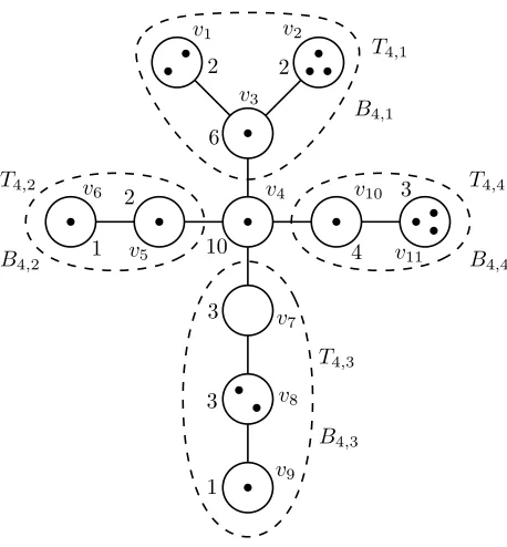
Example. We give a sample tree-decomposition of U11,16. Due to the

sym-metry of the matroid elements, it is not necessary to label the elements of the matroid. We have illustrated the assignment of elements into bags by placing dots within circles. Each dot represents an element in U11,16 and

v1 v2

v3

v4 v10

v6

v5

v7

v8

v9

v11

T4,4

B4,4

B4,2

T4,2

T4,3

B4,3

T4,1

B4,1

2

6 2

4 3 2

1 10

3

3

1

Figure 1: A sample tree-decomposition of the uniform matroidU11,16. Each

circle is labeled by the vertex of the tree that it represents. The dots inside each circle represent the matroid elements that are in the bag corresponding to that vertex. Each circle is also labeled with the node width of its vertex.

widths. Each dashed region indicates a subtree of the treeT and these sub-trees comprise the connected components of the treeT\v4. For example, the

subtreeT4,3 consists of the vertex set {v7, v8, v9} and edge set{v7v8, v8v9}.

As a consequence of each dashed region indicating a connected component of T\v4, the matroid elements within the dashed regions are those of the

subsetsB4,1, B4,2, B4,3andB4,4 ofE(U11,16)−E4displayed by the vertexv4,

whereE4 is the single-element bag associated withv4. To compute the node

width forv4, note that rd(B4,1) = 1 and rd(B4,2) = rd(B4,3) = rd(B4,4) = 0.

Hence nw(v4) =r(U11,16)−1 = 10. Note that this is not an optimal

tree-decomposition ofU11,16. For example, a tree-decomposition whose tree is a

path where each bag contains exactly one matroid element has width six.

W ={x|τ(x)∈V(Tw)}. We say that the edge edisplays the setsU andW. We now prove a lemma that will lend some structure to good tree-decompositions, which we establish in the following corollary.

Lemma 3.1. Let (T, τ) be a tree-decomposition of a matroid M. Suppose that T has an edge e = uw that displays the sets U, W ⊆ E(M), where

U ⊆ cl(W). Then there exists another tree-decomposition (T0_{, τ}0_{) of M} having width at most the width of(T, τ), such that |V(T0_)|<|V(T)|. Proof. Consider T. Let T1, T2, . . . , T` be the connected components of

T\w, where u ∈ T1. Note that U = τ−1(V(T1)). Let T0 be T\T1. We

defineτ0 such that τ0(x) = τ(x) if x /∈U and τ0(x) = w if x ∈U. Clearly,

|V(T0_{)|<|V(T)|. Takes∈V(T}0_{). Ifs6=wthensdisplays the same subsets}

ofE(M) in (T0, τ0) and (T, τ), so nw(T0_,τ0₎(s) = nw_{(T ,τ)}(s).

We conclude this proof by showing that nw(T0_,τ0₎(w) = nw_{(T ,τ)}(w). In the original tree-decomposition, (T, τ), w displays the subsets B1, B2, . . . ,

B`, where Bi = τ−1(V(Ti)). Note that B1 = U. Whereas in (T0, τ0), w

displays the subsets B2, B3, . . . , B`. Since B1 = U ⊆ cl(E(M)−U), we

have rd(B1) = 0. It follows that nw(T0_,τ0₎(w) = nw_{(T ,τ)}(w), as required. The next result follows immediately from Lemma 3.1.

Corollary 3.2. Let M be a matroid with tree-width k. If (T, τ) is a good tree-decomposition ofM, then, for every pair of subsets U and W of E(M)

displayed by an edge ofT, neither r(U) nor r(W) is equal tor(M).

For a good tree-decomposition of a matroid, the preceding result implies that every leaf in the tree corresponds to a set of elements in the matroid that, informally speaking, has some substance. That is, the set is not in the closure of the rest of the elements in the matroid. In the corollary following the next lemma, we bound the rank of such a set of elements.

The following lemma is a collection of fundamental results for tree-width and tree decompositions. The first was proved in [8].

Lemma 3.3. Let M be a matroid. Then (i) tw(M)≥tw(N) if N is a minor of M;

(ii) tw(M) ≤ r(M), where equality holds if M is a projective geometry; and

Proof. Firstly, (i) was proved in [8]. For (ii), consider any tree decomposition (T, τ) of M. By definition of node width, no vertex of T can have node width larger than r(M), thus tw(M) ≤ r(M). In the case where M is a projective geometry, to demonstrate that tw(M) =r(M), it is sufficient to show that a good tree decomposition forM has just one vertex. To that end, suppose thatT has an edge that displaysU ⊆E(M) andW ⊆E(M). Then

{U, W} partitions E(M). However, for every bipartition of the elements of a projective geometry into sets U and W, either r(U) = r(M) or r(W) =

r(M), and it follows from Corollary 3.2 that a good tree decomposition for

M has just one vertex.

To prove (iii), using the notation set up in our definition of tree width, first note that sinceBi,1,...,Bi,ci are a collection of pairwise disjoint subsets ofE(M), by submodularity of the rank function,

r(E(M)−(Bi,1∪Bi,2)) =r((E(M)−Bi,1)∩(E(M)−Bi,2))

≤r(E(M)−Bi,1) +r(E(M)−Bi,2)−r(M).

By repeatedly applying submodularity, we see that

r(E(M)−(Bi,1∪ · · · ∪Bi,ci))≤ ci

X

j=1

r(E(M)−Bi,j)−(ci−1)r(M).

Comparing the rank of the bag of matroid elements Evi associated with vertexvi to the node width ofvi, we have

r(Evi) =r(E(M)−(Bi,1∪ · · · ∪Bi,ci))

≤

ci

X

j=1

r(E(M)−Bi,j)−(ci−1)r(M)

=r(M)−

ci

X

j=1

(r(M)−r(E(M)−Bi,j))

= nw(vi),

as required. In the case wherevi is a leaf ofT, equality holds since nw(vi) =

r(M)−rd(E(M)−Evi) =r(M)−(r(M)−r(Evi)) =r(Evi). The next result follows immediately from Lemma 3.3.

In Corollaries 3.2 and 3.4, we showed that a leaf in the tree of a good tree-decomposition corresponds to a set of elements that has some substance, but not too much substance. We now find a small cocircuit in the matroid, when it is representable over a finite field.

Lemma 3.5. Let M be a simple GF(q)-representable matroid for some prime power q and let M have tree-width k for some positive integer k. ThenM has a cocircuit with at most qk−1 _elements.

Proof. Let (T, τ) be a good tree-decomposition of M. In the case where

v(M) ≥2, T contains a leafw. Let Ew = τ−1(w). By Lemma 3.1, Ew is not contained in the flat clM(E(M)−Ew). Hence this flat is contained in a hyperplane ofM, whose complement is contained inEw. Evidently there is a cocircuit C∗ _{contained in E}

w. Corollary 3.4 implies that Ew has rank at mostk. AsM isGF(q)-representable and simple, we know thatEw is a restriction ofP G(k−1, q). The largest cocircuit inP G(k−1, q) is obtained by deleting a hyperplane, which leavesqk−1 _{elements. Hence|C}∗_{| ≤q}k−1_.

In the case where v(M) = 1, we have r(M) = k ≥ 1, thus M is a restriction of P G(k−1, q). With rank at least 1, M contains a cocircuit, and by the same argument as above,M contains a cocircuitC∗ _with|C∗_{| ≤}

qk−1_.

During the remainder of this paper, for a simple GF(q)-representable matroid M, we denote by Mq the projective geometry P G(r(M)−1, q) of which M is a spanning restriction. If S ⊆ E(Mq)−E(M), then let MS denote the restriction of Mq to the elements of E(M)∪S. Take (T, τ), a tree-decomposition of M. For edgeuw inT, let U0 and W0 be the subsets of E(M) displayed by uw, where τ−1_{(u) ⊆ U}0_{. Let U be the subset of}

elements of Mq obtained by taking the closure clMq(U

0_{), and likewise, let}

W = cl_Mq(W0). We say that the neck of uw with respect to Mq, or simply theneck of uwwhen the projective geometry is clear, is the set of elements in U ∩W. Note that the neck of each edge is a projective geometry over

GF(q). We say that theexternal neck ofuwwith respect toMq, or simply the

external neck ofuwis the intersection of the neck ofuwwithE(Mq)−E(M).

Lemma 3.6. Let (T, τ) be a tree-decomposition of M with width tw(M)

and let S be a subset of the external neck of an edge of T. Then tw(M) = tw(MS_).

E(M) and by letting τ0(x) = u when x /∈E(M). Thus the decomposition is the same except that we add the elements ofS to the bag corresponding tou. (We could equally well add them to the bag corresponding to w.)

We show that, for each edge of T, the corresponding subsets of E(M) andE(MS_{) displayed by this edge have the same rank defects, and conclude} thatM andMS _{have the same tree-width. By the definition of rank defect,} if the elements ofS were added to a set B, then rd_MS(B∪S) = r(MS)−

r_MS(E(M)−B) =r(M)−r_M(E(M)−B) = rd_M(B). Hence the rank defect of B in M is equal to the rank defect of B∪S in MS_{. If the elements of}

S were not added to a set B that is displayed by an edge of T, thenS is a subset of the closure ofE(M)−B inMS _{by construction. The rank defect} again remains unchanged, as rd_MS(B) =r(MS)−r_MS((E(M)−B)∪S) =

r(M)−rM(E(M)−B) = rdM(B). Therefore each vertex inT has the same node width in (T, τ) and (T, τ0). It follows that tw(MS_{) = tw(M).}

Lemma 3.7. Let M be a simple GF(q)-representable matroid with tree-decomposition having tree T. Let uw be an edge of T and suppose that

S={s1, s2, . . . , sn} is the external neck ofuw. Then,

χM(λ) =χMS(λ) + n

X

i=1

χ_M{s₁,s_2,...,si}_/s

i(λ). (2)

Proof. By construction, s1 is neither a loop nor a coloop of Ms1.

Further-more,siis neither a loop nor a coloop ofM{s1,s2,...,si}for alli∈ {1,2, . . . , n}. By Theorem 2.1,χM(λ) =χMs_1/s

1(λ) +χMs1(λ). By repeated application

of Theorem 2.1,

χM(λ) =χMs_1/s

1(λ) +χMs1(λ)

=χMs1/s1(λ) +χM{s₁,s₂}_/s

2(λ) +χM{s1,s2}(λ)

=χ_Ms_1/s

1(λ) +χM{s₁,s2}/s2(λ) +χM{s1,s2,s3}/s3(λ) +χM{s1,s2,s3}(λ)

.. .

=χMs_1/s

1(λ) +χM{s₁,s₂}_/s

2(λ) +· · ·+χMS/sn(λ) +χMS(λ). Thus, the lemma holds.

4

Bounds for zeros of the characteristic

polyno-mial

case where v(M) = 1.

Lemma 4.1. Let M be a loopless, GF(q)-representable matroid of tree-widthk, for some prime powerq and some positive integerk, withv(M) = 1. Suppose that, ifN is a loopless,GF(q)-representable matroid with tree-width at most k and r(N) < r(M), then χN(λ) > 0 for all λ > qk−1. Then

χM(λ)>0 for all λ > qk−1.

Proof. We may assume that M is simple. Let (T, τ) be a good tree-decomposition of M. The single vertex in V(T) must have node width

k. By Lemma 3.3, we have k = r(M). Let S be the set of elements in

E(Mq)−E(M). As in the proof of Lemma 3.7, by repeated application of Theorem 2.1,χM(λ) =χMs_1/s

1(λ) +χM{s₁,s₂}_/s

2(λ) +· · ·+χMS/sn(λ) +

χ_MS(λ). By assumption, each term of this sum is positive for allλ > qk−1 with the possible exception ofχ_MS(λ). AsMSis a projective geometry with rankr(M) =k, it follows thatχ_MS(λ) = (λ−1)(λ−q)(λ−q2)· · ·(λ−qk−1). Thusχ_MS(λ)>0 for allλ > qk−1.

The first proof of the main theorem uses basic tools from characteristic polynomials, and exemplifies the tree-decomposition techniques established by Hlin˘en´y and Whittle in [8], and further developed in this paper, to gen-eralize Thomassen’s graph technique.

Proof of Theorem 1.3. If M has a loop, then its characteristic polynomial is identically zero, so we may assume that M is loopless. As M and its simplification have the same characteristic polynomial and the same

tree-width, we may assume that M is simple. We proceed by induction on

r(M). Suppose that r(M) = 1. Then M ∼= U1,1 and χM(λ) = λ−1. Thus χM(λ) >0 if λ >1, henceχM(λ) is certainly strictly positive for all

λ > qk−1_.

We now assume r(M) > 1. Take (T, τ), a good tree-decomposition of M. If T has a single vertex, then by Lemma 4.1, the result follows. Thus, we may assume that T contains a leaf w with neighbouru. Let S =

{s1, s2, . . . , sn} be the elements in the external neck of uw. By Lemma 3.6, tw(M) = tw(MS_{) and by Lemma 3.7}

χM(λ) =χMS(λ) + n

X

i=1

χ_M{s₁,s_2,...,si}_/s

i(λ). (3)

r(M)−1. Lemma 3.3 implies that tree-width is not increased by contracting elements. By induction the characteristic polynomial of M{s1,s2,...,si}_/s

i is strictly positive for allλ > qk−1_{, for all i∈ {1,2, . . . , n}.}

It remains to consider χ_MS(λ). Let S0 be the neck of uw, which is contained inMS_{. ClearlyM}S_|S0 ∼_{=P G(r}0_{−1, q) for somer}0_{. LetE}

wbe the bag corresponding tow. LetM1=MS|(Ew∪S0) andM2 =MS\(Ew−S0). Then M1|S0 =M2|S0. By [15, Corollary 6.9.6], S0 is a modular flat inM1.

By [15, Proposition 11.4.15], MS _{is the generalized parallel connection of}

M1 andM2 acrossM1|S0. Since M has tree-width at most k, we know that

r0 =rMS(S0)≤r_MS(E_w∪S0) =r_M(Ew)≤k,

with the last part following from Corollary 3.4. Thus, by Theorem 2.2,

χ_MS(λ) =

χM1(λ)χM2(λ)

χP G(r0_−1,q)(λ).

Using Equation (1), we see that the denominator is strictly positive for allλ > qr0₋₁

. Hence it is strictly positive for allλ > qk−1_{. By Corollary 3.2,}

sinceT has v(M) = v(MS_{) vertices, both M}

1 and M2 have rank less than

r(MS_{) =r(M). By our inductive hypothesis, bothχ}

M1(λ) and χM2(λ) are

strictly positive for all λ > qk−1_{. Thus χ}

MS(λ) > 0 for all λ > qk−1, as required.

It is also possible to generalize the second proof of Theorem 1.2, outlined in the introduction, to matroids representable over a finite field by using the following result of Oxley [14, Lemma 2.7].

Lemma 4.2. Let C∗ _{= {x}

1, x2, . . . , xm} be a cocircuit of M. Let Xi,j =

{x1, x2, . . . , xi−1, xi+1, . . . , xj−1} for all1≤i < j ≤m. Then

χM(λ) = (λ−m)χM\C∗(λ) + m

X

j=2

j−1 X

i=1

χM\Xi,j/xi,xj(λ).

A minor-closed family of matroidsMhas thebounded cocircuit property

if there is a constantf(M) =f such that any simple matroidM inMhas a cocircuit of size at mostf. We now apply Lemma 4.2 to any minor-closed family of matroids with the bounded cocircuit property.

Lemma 4.3. Let M be a minor-closed family of matroids having the bounded cocircuit property with constant f. Then for any M in M, either

Proof. Let M be a matroid in M. We may assume that M is simple and that the result is valid ifr(M) = 1.

We now assume r(M) > 1 and proceed using induction on r(M).

Because M has the bounded cocircuit property, we know that M has

a cocircuit C∗ _{with size at most f. Let C}∗ _{= {x}

1, x2, . . . , x|C∗_|} and let Xi,j = {x1, x2, . . . , xi−1, xi+1, . . . , xj−1} for 1 ≤ i < j ≤ |C∗|. By

Lemma 4.2,χM(λ) is equal to the following

(λ− |C∗|)χ_M\C∗(λ) +

|C∗_|

X

j=2

j−1 X

i=1

χ_M\Xi,j/xi,xj(λ). (4)

Nowr(M\C∗) =r(M)−1 andr(M\Xi,j/xi, xj) =r(M)−2, for all 1≤i <

j ≤ |C∗_{|. By induction, each of the characteristic polynomials appearing}

in (4) is either identically zero or strictly positive for λ > f. Furthermore

M\C∗ is loopless and soχM\C∗(λ)>0 forλ > f. As|C∗| ≤f, we conclude that (λ− |C∗_{|), and hence χ}

M(λ), is strictly positive for allλ > f. We now give the alternate proof of Theorem 1.3.

Second proof of Theorem 1.3. Let Mbe the family of GF(q)-representable matroids with tree-width at mostk. Lemma 3.3 implies thatMis a minor-closed class and Lemma 3.5 implies thatMhas the bounded cocircuit prop-erty with constant qk−1_{. The result now follows from Lemma 4.3.}

5

Generalizing to matroids with the bounded

co-circuit property

The argument in the second proof of Theorem 1.3 may be extended to any family of matroids with the bounded cocircuit property. We show the family of matroids with tree-width at mostkcontaining noU2,2+qminor is one such family by using the following theorem of Kung [11].

Theorem 5.1. Let q be an integer at least two. If M is a simple matroid with rankr having no U2,2+q-minor, then |E(M)| ≤ q

r₋₁ q−1.

We now prove Theorem 1.4, in which we replace the representability condition of Theorem 1.3 with the condition that M contain no long line minor. This generalization was suggested by Geelen and Nelson [5].

Proof of Theorem 1.4. We claim that ifM is simple, has tree-width at most

kand has noU2,2+q minor, then it has a cocircuit of size at most q k₋₁ q−1 . The

result then follows by noting that the class of matroids with tree-width at most k having no U2,2+q minor is a minor-closed class and applying Lemma 4.3.

Once again, we may assume thatM is simple and that the claim is valid ifr(M) = 1. We proceed by induction on r(M). Take (T, τ), a good tree-decomposition ofM and vertexv∈V(T) with degree at most one. Let Ev be the bag corresponding to v and let r = r(Ev). Lemma 3.3(iii) implies thatr ≤k. If T consists of a single vertex, thenE(M) =Ev. Furthermore

Evcontains a cocircuit sincer ≥1. Suppose then thatT contains more than one vertex. Thenvis a leaf vertex. Since (T, τ) is a good tree-decomposition,

Ev is not contained in cl(E(M)−Ev) by Lemma 3.1. Thus Ev contains a cocircuit ofM.

Theorem 5.1 implies that |Ev| ≤ q r₋₁ q−1 ≤

qk−1

q−1 . Thus M has a cocircuit

C∗ _{of size at most} qk₋₁ q−1 .

In Corollary 1.5, we completely determine whether there is a bound on the largest real root of the characteristic polynomial of any matroid belonging to a minor-closed family having bounded tree-width. It would be interesting to find minor-closed classes of matroids that do not have the bounded cocircuit property and determine bounds on the real characteristic roots.

Acknowledgements

We thank the anonymous referees, Jim Geelen and Peter Nelson for several helpful comments.

References

[2] Brylawski, T. Modular constructions for combinatorial geometries.

Transactions of the American Mathematical Society 203, 1–44 (1975).

[3] Brylawski, T., and Oxley, J. The Tutte polynomial and its applications.

Matroid Applications, Encyclopedia of Mathematics and its Applica-tions40, 123–225. Cambridge University Press, Cambridge (1992).

[4] Dong, F., Koh, K., Teo, K.Chromatic polynomials and chromaticity of graphs, World Scientific Publishing Company, Singapore (2005).

[5] Geelen, J., and Nelson, P. Private communication (2014).

[6] Geelen, J. and Nelson, P. The number of points in a matroid with no

n-point line as a minor.Journal of Combinatorial Theory Series B100

625–630 (2010).

[7] Haggard, G., Pearce, D. J., and Royle, G. F. Computing Tutte poly-nomials. ACM Transactions on Mathematical Software 37, 24:1–24:17 (2010).

[8] Hlin˘en´y, P. and Whittle, G. Matroid tree-width. European Journal of Combinatorics27, 1117–1128 (2006).

[9] Jackson, B. A zero-free interval for chromatic polynomials of graphs.

Combinatorics, Probability and Computing 2, 325–336 (1993).

[10] Jacobsen, J. L., and Salas, J. Is the five-flow conjecture almost false?

Journal of Combinatorial Theory Series B 103, 532–565 (2013).

[11] Kung, J. P. S., Extremal matroid theory,Graph Structure Theory (Seat-tle WA, 1991), Contemporary Mathematics,147, American Mathemat-ical Society, Providence RI, 1993, 21–61 (1993).

[12] Mader, W. Homomorphieeigenschaften und mittlere Kantendichte von Graphen.Mathematische Annalen 174, 265–268 (1967).

[13] Nelson, P. The number of rank-kflats in a matroid with noU2,n-minor. Journal of Combinatorial Theory Series B 107, 140–147 (2014).

[14] Oxley, J. Colouring, packing and the critical problem.Quart. J. Math. 29, 11–22 (1978).

[16] Robertson, N., and Seymour, P. D. Algorithmic aspects of tree-width.

Journal of Algorithms 7, 309–322 (1986).

[17] Royle, G. F. Recent results on chromatic and flow roots of graphs and matroids.Surveys in Combinatorics, London Mathematical Society Lecture Note Series 365, 289–327. Cambridge University Press, Cam-bridge (2009).

[18] Sokal, A. D. Bounds on the complex zeros of (di)chromatic polynomials and Potts-model partition functions. Combinatorics, Probability and Computing 10, 41–77 (2001).

[19] Sokal, A. D., Chromatic roots are dense in the whole complex plane.

Combinatorics, Probability and Computing,13221–261 (2004).

[20] Thomassen, C. The zero-free intervals for chromatic polynomials of graphs. Combinatorics, Probability and Computing 6, 497–506 (1997).

[21] Woodall, D. R. The largest real zero of the chromatic polynomial. Dis-crete Mathematics 172, 141–153 (1997).

[22] Zaslawsky, T., The M¨obius function and the characteristic polynomial.