Evolution of the Contact Area with Normal Load for Rough Surfaces: from Atomic to Macroscopic Scales

N A N O E X P R E S S

Open Access

Evolution of the Contact Area with Normal

Load for Rough Surfaces: from Atomic to

Macroscopic Scales

Shiping Huang

Abstract

The evolution of the contact area with normal load for rough surfaces has great fundamental and practical importance, ranging from earthquake dynamics to machine wear. This work bridges the gap between the atomic scale and the macroscopic scale for normal contact behavior. The real contact area, which is formed by a large ensemble of discrete contacts (clusters), is proven to be much smaller than the apparent surface area. The distribution of the discrete contact clusters and the interaction between them are key to revealing the mechanism of the contacting solids. To this end, Green’s function molecular dynamics (GFMD) is used to study both how the contact cluster evolves from the atomic scale to the macroscopic scale and the interaction between clusters. It is found that the interaction between clusters has a strong effect on their formation. The formation and distribution of the contact clusters is far more complicated than that predicted by the asperity model. Ignorance of the interaction between them leads to overestimating the contacting force. In real contact, contacting clusters are smaller and more discrete due to the interaction between the asperities. Understanding the exact nature of the contact area with the normal load is essential to the following research on friction.

Keywords:Fractal surface, Asperity model, Green’s function molecular dynamics, Contact area

Background

Most macroscopic surfaces are considered to be rough and fractal [1, 2]. The contact behavior between rough surfaces is much more complicated than that of perfectly smooth surfaces [3, 4]. The real contact area is formed by a large ensemble of discrete contact regions (clusters), which is much smaller than the apparent surface area. The normal force and the size, shape, and distribution of the contact clusters are key to revealing the contact be-havior, which is essential for the following studies on friction [5–7].

To obtain the relationship between the contact area and the load, numerous models have been proposed since the 1960s [1, 8–14]. Among them, the asperity model is the simplest and most popular one. In one of the early applications of the asperity model, Greenwood

and Williamson [8] describe the roughness of the con-tact interface by assuming that asperities have the same radii but different heights. Since then, the asperity model has prevailed and a vast amount of literature has appeared in this field. Whitehouse and Archard [15] developed the Greenwood and Williamson (G-W) model by accounting for the random radii of curvature of the asperity tips. Nayak [16–18] introduced the techniques of random process theory [19, 20] into the analysis of Gaussian roughness, which was subsequently used by Bush et al. [9] in rough surface contact.

One of the basic assumptions in the asperity model is that the interaction between the asperities can be neglected, which indicates that the potential contact asperities can be determined by the surface geometry in advance. However, this assumption may lead to inaccur-ate estimations of the contact force and contact area. To obtain the evolution of the contacting clusters and the interaction between them, we utilize Green’s function molecular dynamics (GFMD) [21–23] to study the fractal rough surface.

Correspondence:[email protected]

1

School of Civil Engineering and Transportation, South China University of Technology, Guangzhou 510640, People’s Republic of China

2_{State Key Laboratory of Coal Resources and Safe Mining, China University of}

Mining and Technology, Xuzhou 221116, Jiangsu, People’s Republic of China Full list of author information is available at the end of the article

This work is to bridge the gap between the atomic scale and the macroscopic scale for normal contact behavior. The evolution of the contact area from atomic to macroscopic scales is demonstrated through numer-ical examples with the consideration of the asperity interactions. In the subsequent discussion, we first briefly present our approaches for the fractal surface generation, the GFMD model, the contacting cluster detection algorithm, and the numerical experimental design. We then focus on the forming and development of the contacting cluster and the influence of these processes on the interface’s behaviors.

Methods

Rough Fractal Surface Generation

To study the contact behavior of the rough surface, we need to generate the surface for the numerical model. Several algorithms have been used for fractal surfaces [24]. In this work, we use the Fourier transform method to generate fractal rough surfaces, as seen in Fig. 1. Four parameters are required to determine the fractal rough surface geometry. These are the maximum frequency (wH), the minimum frequency (wL), the Hurst exponent

(H), and the standard deviation of the amplitude (P). The surface’s basic statistical parameters, such as RMS (root mean square) height pffiffiffiffiffiffiffiM0, RMS slope pffiffiffiffiffiffiffiM2,

and RMS curvature pffiffiffiffiffiffiffiM4, are the key parameters for

the interface’s behaviors, where Mi is the ith radial

moment of the surface spectrum [19, 20]. It is worth noting that the surface statistical parameterMiis related

to the profile statistical parameters mi by the following

equation: M0¼m0;M2¼2m2;M4¼43m4 . It is well known that the asperity density n (surface summits or valleys) can be determined by the following equation:

n¼ 1

6πpffiffiffi3ðm4=m2Þ ð1Þ

Additionally, the surface total summit/valley number Nis expressed by

N¼A0n¼A0 1

6πpffiffiffi3ðm4=m2Þ ð2Þ whereA0is the apparent surface area. For the self-affine

fractal surface, the surface statistical parameters are related to the input parameters (w,H,P) by the following equation:

mi¼

Z _wH

wL

ωi_{Φϕð Þω dω¼}

Z _wH

wL

ωi_Bω−ð1þ2HÞ_{dω ð3Þ}

where B is the surface roughness constant, which is related to P. Equations (3) and (2) indicate that the fractal surface summit/valley number is dependent on the wavelength and the Hurst exponent. Detailed discussions

of the fractal surface statistical properties can be found in the literature [25,26].

In the Fourier transform algorithm, as a typical example, we set the Hurst component to beH= 0.5, the maximum frequency to be wL= 1/(24σ), the minimum

frequency to bewH= 1/(256σ), the standard deviation of

the frequency amplitude to be P= 0.69, and the system size to be 512 × 512 atoms (with initial spacing equal to 1.12σ). These input parameters subsequently generate the surface with the following statistical parameters: sur-face RMS slopepffiffiffiffiffiffiffiM2¼0:077 and RMS curvature pffiffiffiffiffiffiffiM4

¼0:0077 . The total number of surface summits/valleys is 150 based on Eq. (2), while by counting the number numerically, the surface summit number is 158 and the valley number is 159. The error is within 5%, which sug-gests that the system size is acceptable in a statistical sense. In fact, when we increase the system size up to 2048 × 2048 atoms (with initial spacing equal to 1.12σ), the results for the statistical parameters are consistent with those of the smaller system.

GFMD Model

Inter-particle interaction is very difficult to capture experimentally [6, 27]. Recently, molecular dynamics has been used to simulate inter-particle interaction, aiming to investigate the molecular origins of the contact/friction mechanism. However, the computational expense is con-siderably high for large-scale molecular dynamics simula-tions. Therefore, GFMD is introduced to simulate the surface due to its high efficiency. GFMD uses molecular dynamics to simulate the interaction of the interface’s atoms (two layers here), while the non-interface layer, which usually exhibits elastic behaviors, is simulated by the Green’s function. Thus, it reduces the large atomic system to two-layer atoms at the interface (as seen in Fig. 1), which dramatically reduces the computational expense. Detailed discussions of GFMD can be seen in the literature [21–23, 28]. In the GFMD model, the Lennard-Jones (LJ) potential is used to simulate the inter-particle interaction. The equation is written as

u rð Þ ¼4ε σ r 12 − σ r 6

ð4Þ

whereε is the depth of the potential well,σ is the finite distance at which the inter-particle potential is zero, and ris the distance between the particles. We takeε,σ, and

ε/σ as the energy, distance unit, and force unit, respect-ively. According to the LJ potential, we know that when r= 21/6σ≈1.12σ, the inter-particle force is zero. When r> 1.12σ, the inter-particle force is attractive; when r< 1.12σ, the inter-particle force is repulsive. Since we do not consider adhesion in this work, the cutoff distance is set to be 1.12σ. The crystal structure used for the atomic

layer is face-centered cubic (FCC). Due to symmetry, we only take the interface’s layer to form the surface geom-etry as shown in Fig. 1, and the elastic block below the flat surface is simulated by Green’s function.

Contacting Cluster Recognition Method

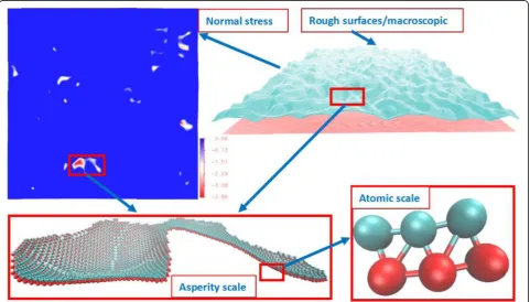
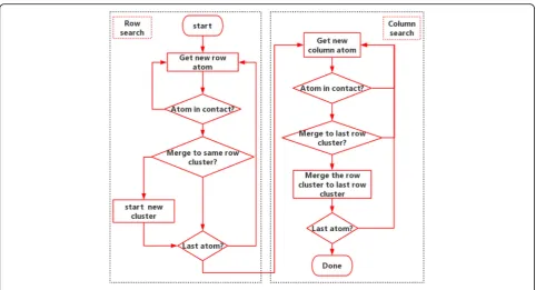
There are three scales observed in the interface as seen in Fig. 1: (1) atomic scale, which is simulated by LJ potential; (2) asperity scale, which is the group effect of contact atoms; and (3) macroscopic scale, which is the group effect of contact clusters. The size, shape, location, and distribution of the contact clusters are the critical bridge between molecular behavior and interface properties. At the nanoscale, the atomic contact region is difficult to define [6]. We here define a contact atom by its normal component force fz > 0. Subsequently, the connected con-tacting atoms are defined as a concon-tacting cluster. The labeling technique [29, 30] is used to search the contacting cluster. Here, we use a modified algorithm for acceler-ation, which avoids the recursive searching process. The algorithm flow chart is shown in Fig. 2, where atomic force data are extracted from the Green’s function mo-lecular dynamics simulation. The algorithm is divided into eight key steps as follows.

Step 1. Start the row search and get the new atom data, that is, search the atoms from row to row.

Step 2. Determine if the atom is in contact. If it is not in contact, go back to step 1. If it is in contact, move to the next step.

Step 3. Compare the current atom with the previous atom in the same row. If the previous atom is also in contact, merge the atom into the cluster to which the previous atom belongs, then label the atom with the same number as the previous atom. If the previous atom is not in contact, label the atom with a new number that is the previous number plus one.

Step 4. Determine whether it is the last atom; if not, go back to step 1, or go to the column search process.

Step 5. Start the column search and get the new atom data, that is, search the atoms from column to column.

Step 6. Determine if the atom is in contact. If it is not in contact, go back to step 5. If it is in contact, move to the next step.

Step 7. Compare the current atom with the previ-ous atom in the same column. If the previprevi-ous atom is also in contact and belongs to a different cluster, merge the current cluster into the cluster to which the previous atom belongs, then label the atoms with the same number and store them. If the previous atom is not in contact or belongs to the same cluster, move to the next step.

Numerical Experimental Design

It is well known that two-rough surface contact problem can be simplified as a problem with one composite rigid rough surface and a flat elastic surface by introducing the equivalent elastic modulusE*, which is written as

1 E¼

1−v2 1 E1 þ

1−v2 2

E2 ð

5Þ

where E1 and E2 are the elastic modulus of the upper

surface and the lower surface, respectively. For simpli-city, we consider a rigid rough surface contacting with an elastic smooth surface and then study the formation and development of the contacting cluster and its force-area behavior. In the following discussion, we will use the surface generated above (the upper surface is rigid and rough (E1=∞), and the lower surface is smooth and

elastic (E2= 3ε/σ3)) to study the contact behavior, where

both of v1and v2 are set to be 0.5. Our system size is

512 × 512 atoms (with initial spacing equal to 1.12σ), and periodic boundary conditions are used in the x-y plane. The elastic block depth is set to be 1024 atomic layers (with initial spacing equal to 1.12σ). In a regular molecular dynamics simulation, the system will be com-prised of 268,697,600 atoms; the GFMD model reduces the number to 524,288 (two layers of atoms), as seen in Fig.1. We gradually push the rough surface (on the top) into the flat elastic surface. The loading of the rigid surface is controlled by the displacement. Each displacement load-ing step is set to 0.01σ, and the GFMD algorithm will

update each atom’s position until the atomic force meets the convergence criteria L1-norm = 0.01ε/σ. The maximum iteration number is set to be 50,000 to avoid an endless loop.

Results and Discussion

Contacting Clusters’Distribution and Development

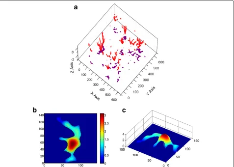
The asperity model considers the asperity to be either spherical or elliptical and does not consider the inter-action between the contacting asperities. In this work, the asperities used in asperity model are extracted from the surface generated above. In the asperity model, the potential contacting asperities can be determined by the surface geometry in advance based on their heights; that is, the surface summits/valleys will form as contact clus-ters according to their heights. However, in reality, the asperity has an irregular shape, and usually, several adja-cent asperities may merge into a big one, as shown in Fig. 2. It is observed that there are six independent asperities at the beginning, and as the contact force increases, they finally merge into a big contacting cluster (Fig. 3). This suggests that the assumption that the inter-asperity distance is far enough for asperities to not affect one another may lead to inaccurate results.

Figure 4 demonstrates that the cluster number first increases and then decreases as the contact area increases, while the surface asperity always increases as the contact area increases. This is due to the merging effect explained in Fig. 3.

a

b

c

Fig. 3The shape of the clusters and the merging effect.aThe 3D view of contact clusters and its projection on thex-yplane (inσ).bA typical contact cluster comprising of six independent asperities.cThe 3D view of the contact cluster’s geometry (inσ)

Fig. 4Surface valleys and cluster number under different

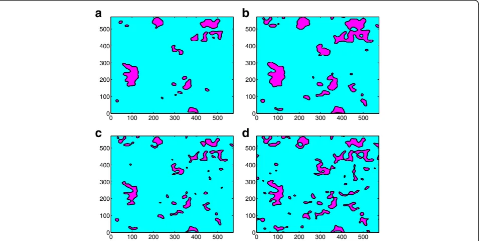
The contact cluster merging effect has been observed in both the asperity model and the GFMD model. How-ever, with the same contact area, the contact cluster number in the GFMD model is much larger than that of the asperity model, as seen in Fig. 5. It is observed that the number of contact clusters in the GFMD model is almost twice that in the asperity model, as shown in Fig. 5. The main reason for this is that the asperity model does not consider the inter-asperity interaction. However, in the GFMD model, the contact clusters influence each other. The displacement fields gener-ated by the contact clusters are continuous all over the surface area. The displacement of the large en-semble of clusters results in a new geometry on the elastic surface, which affects the formation of new contact clusters. Therefore, the formation of the con-tact cluster not only is based on the height of the rigid rough surface but also can be influenced by de-formations in the smooth elastic surface. This can also be observed in Fig. 6, which shows the contact cluster distribution at different areas for the asperity model and GFMD model, respectively. As shown in Fig. 6, at a contact area of 5%, contact cluster num-bers are 17 and 34 for the asperity model and the GFMD model, respectively, while at a contact area of 10%, their contact cluster numbers become 24 and 52, respectively. This suggests that the contact clus-ters in GFMD model are more discrete than those in the asperity model. In the GFMD model, the average cluster size is smaller, but most of the clusters will

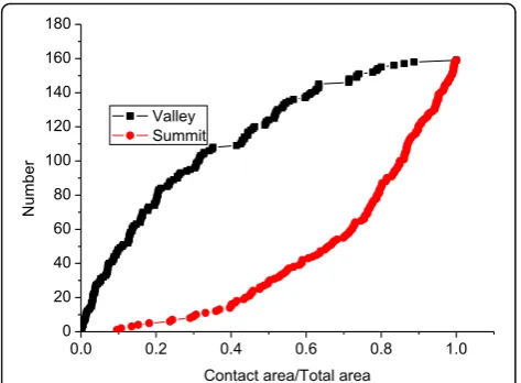
coincide with the summits/valleys, as can be observed in Fig. 7. Furthermore, the asperity model considers either the valleys or the summits as potential asper-ities (depending on which side is in contact). How-ever, in Fig. 8, we found that as the contact area increases, both of the summits and the valleys can be in contact. In Fig. 8, most asperities in contact are the surface valleys when the contact area is small. However, when the contact area is larger than 10% of the surface area, more and more summits can also form as the contact clusters.

a

b

c

d

Fig. 6The cluster distribution contour (inσ) at different contact areas for the asperity model and GFMD model, respectively.aAsperity model with 5% contact area.bAsperity model with 10% contact area.cGFMD model with 5% contact area.dGFMD model with 10% contact area

Contact Area-Load Relationship

The force-area relationship under a normal load is essential to the contact behavior. In the earlier models, asperities are usually considered to be spherical and elliptical. However, real contact clusters are much more complicated. In this section, we compared three models’ contact force-area relationship: (1) the GFMD model; (2) the asperity model (marked as AM), in which the asper-ity is directly extracted from the surface before we use GFMD to push those asperities into the flat elastic surface (this ensures that there is no unexpected contact cluster formation during the contact); and (3) the Green-wood and Williamson model (marked as G-W), in which the asperity is converted to the equivalent sphere. The sphere radius is obtained by

1 R¼

8 3

m4

π

1=2

ð6Þ

For the GFMD model and the asperity model with as-perities extracted exactly from the surface, the total forces in the interface can be obtained by summing each contact cluster’s forces extracted from GFMD. For the Greenwood and Williamson model, we use the Hertz theory for each asperity force (with the same material property used in the GFMD model), which means that the total forceFcan be expressed as

F¼X

n

i¼1 fi¼

XN

i¼1 4 3E

_R1=2_ðd−ziÞ3=2 _ð 7Þ

where Zi is the asperity height, d is the displacement applied at the rigid surface, andfis the asperity contact force based on the Hertz contact theory.

In Fig. 9, we compared the three models’ force-area relationships, which exhibit linear relations. It is observed that the total force in GFMD is much smaller than that of the asperity model and the G-W model. F

in the asperity model is 1.80 times than that predicted by GFMD, and F in the G-W model is 1.54 times than that predicted by GFMD. This can be explained by the RMS slope of the contact clusters. It is known that the normal load is proportional to the RMS slope, that is, L

∝pffiffiffiffiffiffiffiM2. In the GFMD model, the contact area is com-posed of a greater number of clusters, whose penetra-tions are shallower than that of the asperity model. Since the asperity tip’s slope is smaller, the RMS slope for the contact cluster in the GFMD model is also smaller. Figure 10 shows the contact cluster’s RMS slopes for the three models. It can be seen that the contact clusters’ RMS slope in GFMD is less than that of surface RMS slope of 0.077, while both of the other two models’contact cluster RMS slopes are larger than that of the surface RMS slope.

Fig. 8The surface valley and summit numbers grow at different areas

Conclusions

To find the evolution of the contact area from atomic scale to macroscopic scale, the rough fractal surface contact problem has been studied using the GFMD model. We defined the atomic contact by the existence of a force larger than zero and studied three different length scales in the same system. It is found that the inter-asperity interaction is essential to the forming of a contact cluster. Some clusters are close enough that they can merge into a big one. The real contact region is far more complicated than that predicted by surface geom-etry due to elastic deformation in the elastic smooth surface. Most of the contact cluster locations are coincident with the surface summits/valleys. However, the cluster’s size is smaller, and its formation is not determined by the sur-face asperity heights. As the contact area increases, both summits and valleys can form as contact clusters. In the GFMD model, the force is much smaller than that of the asperity model, while the contact cluster number in the GFMD model is much larger. The RMS slope of the con-tact clusters in the GFMD model is smaller than that of the asperity model, which explains why the asperity model leads to higher pressure. Our findings suggest that the real contact area cannot be predicted simply by the surface geometry. The actual contact area with the normal load is of importance for the following research on friction.

Acknowledgements

Shiping Huang thanks Mark O. Robbins (Johns Hopkins University), Tristan A. Sharp (University of Pennsylvania), and Lars Pastewka (Albert-Ludwigs-Universität Freiburg) for providing the GFMD codes and many useful discussions during his postdoctoral research at the Department of Physics and Astronomy, Johns Hopkins University.

Funding

This material is based on the work supported by the National Natural Science Foundation of China under Grant Nos. 11202080 and11672108 and supported by“the Fundamental Research Funds for the Central Universities”. Part of this work is funded by the Research Fund of The State Key Laboratory of Coal Resources and Safe Mining, CUMT (12KF07).

Competing Interests

The author declares no competing interests.

Publisher’s Note

Springer Nature remains neutral with regard to jurisdictional claims in published maps and institutional affiliations.

Author details 1

School of Civil Engineering and Transportation, South China University of Technology, Guangzhou 510640, People_’s Republic of China.2_{State Key}

Laboratory of Coal Resources and Safe Mining, China University of Mining and Technology, Xuzhou 221116, Jiangsu, People’s Republic of China.3_State

Key Laboratory of Tribology, Tsinghua University, Beijing 100084, People’s Republic of China.4_{Department of Physics and Astronomy, Johns Hopkins}

University, 3400 North Charles Street, Baltimore, MD 21218, USA.

Received: 22 August 2017 Accepted: 3 November 2017

References

1. Huang S, Misra A (2013) Micro_–macro shear-displacement behavior of contacting rough solids. Tribol Lett 51(3):431–436

2. Hyun S, Pei L, Molinari J-F, Robbins M (2004) Finite-element analysis of contact between elastic self-affine surfaces. Phys Rev E 70(2):026117 3. Peng Z, Chen S (2011) Effects of surface roughness and film thickness on

the adhesion of a bioinspired nanofilm. Phys Rev E 83(5):8 4. Luan B, Robbins MO (2005) The breakdown of continuum models for

mechanical contacts. Nature 435(7044):929_–932

5. Ben-David O, Rubinstein SM, Fineberg J (2010) Slip-stick and the evolution of frictional strength. Nature 463(7277):76–79

6. Mo Y, Turner KT, Szlufarska I (2009) Friction laws at the nanoscale. Nature 457(7233):1116_–1119

7. Stelmakh AU, Pilgun YV, Kolenov SO, Kushchev AV (2014) Reduction of friction and wear by grooves applied on the nanoscale polished surface in boundary lubrication conditions. Nanoscale Res Lett 9(1):226

8. Greenwood JA, Williamson JB (1966) Contact of nominally flat surfaces. Proc R Soc London, Ser A. 295(1442):300–319

9. Bush AW, Gibson RD, Thomas TR (1975) Elastic contact of a rough surface. Wear 35(1):87–111

10. Majumdar A, Bhushan B. Fractal model of elastic-plastic contact between rough surfaces. J Tribol-T Asme 1991;113(1):1-11

11. Persson BNJ, Albohr O, Creton C, Peveri V (2004) Contact area between a viscoelastic solid and a hard, randomly rough, substrate. J Chem Phys 120(18):8779_–8793

12. Greenwood JA (2006) A simplified elliptic model of rough surface contact. Wear 261(2):191–200

13. Persson BNJ (2007) Relation between interfacial separation and load: a general theory of contact mechanics. Phys Rev Lett 99(12):125502 14. Zavarise G, Paggi M (2008) Reliability of micromechanical contact models: a

still open issue. In: Wriggers P, Laursen TA (eds) CISM International Centre for Mechanical Sciences. CISM, Udine, Vienna, p 498

15. Whitehouse DJ, Archard JF (1970) Properties of random surfaces of significance in their contact. Proc R Soc London, Ser A 316(1524):97–121 16. Nayak PR (1973) Some aspects of surface-roughness measurement. Wear

26(2):165–174

17. Nayak PR (1973) Random process model of rough surfaces in plastic contact. Wear 26(3):305–333

18. Nayak PR (1971) Random process model of rough surfaces. J Lubr Technol 93(3):398–407

19. Longuet-Higgins MS (1957) Statistical properties of an isotropic random surface. Philos Tr R Soc S-A. 250(975):157–174

20. Longuet-Higgins MS (1957) The statistical analysis of a random, moving surface. Philos Tr R Soc S-A 249(966):321–387

21. Pastewka L, Sharp TA, Robbins MO (2012) Seamless elastic boundaries for atomistic calculations. Phys Rev B 86(7):075459

22. Campañá C (2008) Using Green’s function molecular dynamics to rationalize the success of asperity models when describing the contact between self-affine surfaces. Phys Rev E 78(2):026110

23. Campaná C, Müser MH (2006) Practical Green’s function approach to the simulation of elastic semi-infinite solids. Phys Rev B 74(7):075420 24. Peitgen H-O, Saupe D, Barnsley MF, Fisher Y, McGuire M. The science of

fractal images: Springer New York etc.; 1988

25. Zavarise G, Borri-Brunetto M, Paggi M (2007) On the resolution dependence of micromechanical contact models. Wear 262(1–2):42–54

26. Sayles RS, Thomas TR (1978) Surface-topography as a nonstationary random process. Nature 271(5644):431_–434

27. Cai W, Fan H, Zhao J, Shang G (2014) Real-time deflection and friction force imaging by bimorph-based resonance-type high-speed scanning force microscopy in the contact mode. Nanoscale Res Lett 9(1):665

28. Huang S, Wu J, Hu J, Zheng H, Wang W (2017) Numerical analysis of asperity contact model based on molecular dynamics-Green’s function method. Chinese Journal of Theoretical and Applied Mechanics 49(4):961–967 29. Hoshen J, Kopelman R (1976) Percolation and cluster distribution. I. Cluster

multiple labeling technique and critical concentration algorithm. Phys Rev B 14(8):3438