Adaptive models and heavy tails with an application to inflation forecasting

BIROn - Birkbeck Institutional Research Online

Delle Monache, D. and Petrella, Ivan (2016) Adaptive models and heavy

tails with an application to inflation forecasting. Working Paper. Birkbeck,

University of London, London, UK.

Downloaded from:

Usage Guidelines:

Please refer to usage guidelines at or alternatively

ISSN 1745-8587

BCAM 1603

Adaptive models and heavy tails with an

application to inflation forecasting

Davide Delle Monache

Bank of Italy

Ivan Petrella

WBS and CEPR

November 2016

Birkb

eck

C

e

ntre fo

r

Ap

plie

d

Mac

roecono

Adaptive models and heavy tails with an

application to inflation forecasting

∗

Davide Delle Monache

Bank of Italy

Ivan Petrella

WBS and CEPR

November, 2016

Abstract

This paper introduces an adaptive algorithm for time-varying autoregressive models

in the presence of heavy tails. The evolution of the parameters is determined by the score

of the conditional distribution, the resulting model is observation-driven and is estimated

by classical methods. In particular, we consider time variation in both coefficients and

volatility, emphasizing how the two interact with each other. Meaningful restrictions are

imposed on the model parameters so as to attain local stationarity and bounded mean

values. The model is applied to the analysis of inflation dynamics with the following

results: allowing for heavy tails leads to significant improvements in terms of fit and

forecast, and the adoption of the Student-t distribution proves to be crucial in order to

obtain well calibrated density forecasts. These results are obtained using the US CPI

inflation rate and are confirmed by other inflation indicators, as well as for CPI inflation

of the other G7 countries.

JEL classification: C22, C51, C53, E31.

Keywords: adaptive algorithms, inflation, score-driven models, student-t,

time-varying parameters.

∗_{The views expressed in this paper are those of the authors and do not necessarily reflect those of Banca} d’Italia. The authors would like to thank Michele Caivano, Ana Galvao, Anthony Garratt, Emmanuel Guerre, Andrew Harvey, Dennis Kristensen, Haroon Mumtaz, Zacharias Psaradakis, Barbara Rossi, Emiliano Santoro, Tatevik Sekhposyan, Ron Smith, Brad Speigner and Fabrizio Venditti for their useful suggestions. We also thank the participants at the workshop “Economic Modelling and Forecasting - Warwick Business School, 2013”, the EABCN Conference “Inflation Developments after the Great Recession - Eltville, 2013”, the “7th International Conference on Computational and Financial Econometrics - London, 2013”, the workshop on “Dynamic Models driven by the Score of Predictive Likelihoods - Tenerife, 2014”, the “IAAE Annual Conference - London, 2014”, the “25th EC2 Conference Advances in Forecasting - Barcelona, 2014”, the “European Winter Meeting of the Econometric Society - Madrid, 2014”, and the seminar participants at Queen Mary University, University of Glasgow, Bank of England and Banca d’Italia.

1

Introduction

In the last two decades there has been an increasing interest in models with time-varying parameters (TVP) for the analysis of macroeconomic variables. Stock and Watson (1996) have

renewed the interest in this area by documenting the widespread forecasting gains of TVP

models.1 _{Recently, Cogley and Sargent (2005), Primiceri (2005), Stock and Watson (2007)}

have highlighted the importance of allowing for time variation in the volatility as well as in the

coefficients.2 _{Yet, most of the studies so far have considered TVP models under the assumption}

that the errors are Normally distributed. Although this assumption is convenient, it limits the

ability of the model to capture the tail behavior that characterizes a number of macroeconomic

variables. As the recent recession has shown, departures from Gaussianity are important so as

to properly account for the risks associated with black swans (see, e.g., C´urdia et al. 2014).

This paper considers an adaptive autoregressive model where the errors are Student-t

dis-tributed. Following Creal et al. (2013) and Harvey (2013), the parameters’ variation is driven

by the score of the conditional distribution. In this framework, the distribution of the

innova-tions not only modifies the likelihood function (as, e.g., in the t-GARCH of Bollerslev, 1987),

but also implies a different updating mechanism for the TVP. In this regard, Harvey and

Chakravarty (2009) highlight that the score-driven model for time-varying scale with

Student-t innovaStudent-tions leads Student-to a filStudent-ter Student-thaStudent-t is robusStudent-t Student-to ouStudent-tliers, while Harvey and LuaStudent-ti (2014) show

that the same intuition holds true in models with time-varying location. The resulting model

is observation-driven. As opposed to parameter-driven models, the parameters’ values are ob-tained as functions of the observations only, the likelihood function is available in closed form,

and thus the model is estimated by classical methods.3

As stressed by Stock (2002) in his discussion of Cogley and Sargent (2002), estimating TVP

models without controlling for the possible heteroscedasticity is likely to overstate the time

variation in the coefficients (see also Benati, 2007). In this paper, we consider time variation

in both coefficients and volatility, emphasizing how the two interact with each other in a

score-driven model. Moreover, we show how to impose restrictions on the model’s parameters so as

to achieve local stationarity and bounded long-run mean. Both restrictions, commonly used in

applied macroeconomics, have not yet been considered in the context of score-driven models. The adaptive model in this paper is related to an extensive literature that has investigated

ways of improving the forecasting performance in presence of instability. Pesaran and

Tim-merman (2007), Pesaran and Pick (2011) and Pesaran et al. (2013) focus on optimal weighting

scheme in the presence of structural breaks. Giraitis et al. (2014) propose a non-parametric

estimation approach of time-varying coefficient models. The weighting function implied by

these models are typically monotonically decreasing with time, a feature which they share with

1_{Attempts to take into account the well-known instabilities in macroeconomic time series can be traced}

back to Cooley and Prescott (1973, 1976), Rosenberg (1972), and Sarris (1973).

2_{D’Agostino et al. (2013) highlight the relative gains in terms of forecast accuracy of TVP models compared}

to the traditional constant parameter models in a multivariate setting.

3_{In the parameter-driven models the dynamics of the parameters is driven by an additional idiosyncratic}

traditional exponential weighted moving average forecasts (see e.g. Cogley, 2002). Our model

features time variation in location and scale, and Student-t errors. This implies a non-linear

filtering process with a weighting pattern that cannot be replicated by the procedures proposed

in the literature. The benefit of this approach is that observations that are perceived as out-liers, based on the estimated conditional location and scale of the process, have effectively no

weight in updating the TVP. The resulting pattern of the weights is both non-monotonic and

time-varying since it is a function of the estimated TVP. Therefore, the model implies a faster

update of the coefficients in periods of high volatility. Furthermore, in periods of low volatility,

even deviations from the mean that are not extremely large in absolute terms are more likely

to be ‘classified’ as outliers. As such, they are disregarded by the filter, which is robust to

extreme events. Those model’s features are important in the analyis of macroeconomic time

series that display instability and changes in volatility. This is demonstrated empirically with

an application to inflation dynamics.

Understanding inflation dynamics is key for policy makers. In particular, modern

macroe-conomic models highlight the importance of forecasting inflation for the conduct of monetary

policy (see e.g. Svensson, 2005). There are at least three reasons why our model is

particu-larly suitable for inflation forecasting. First, simple univariate autoregressive models have been

shown to work well in the context of forecasting inflation (see Faust and Wright, 2013). Second,

Pettenuzzo and Timmermann (2015) show that TVP models outperform constant-parameters

models and that models with small/frequent changes, like the model proposed in this paper,

produce more accurate forecasts than models whose parameters exhibit large/rare changes.

Third, while important changes in the dynamic properties of inflation are well documented (see e.g. Stock and Watson, 2007), most of the empirical studies are typically framed in a

Bayesian setup and present a number of shortcomings: (i) it is computationally demanding;

(ii) when restrictions are imposed to achieve stationarity, a large number of draws need to be

discarded, therefore leading to potentially large inefficiency4_{; (iii) Normally distributed errors}

are usually assumed. The latter point is particularly relevant as it is well known, at least

since the seminal work of Engle (1982), that the distribution of inflation displays non-Gaussian

features. The adaptive model presented in this paper tackles all these shortcomings.

When used to analyze inflation, our model produces reasonable patterns for the long-run

trend and the underlying volatility. By introducing the Student-t distribution, we make the

model more robust to short lived spikes in inflation (for instance in the last part of the sam-ple). At the same time, the specifications with Student-t innovation display substantially more

variation in the volatility. In practice, with Student-t innovations the variance is less affected

by the outliers and it can conveniently adjust to accommodate changes in the dispersion of

the central part of the distribution. The introduction of heavy tails improves the fit and the

out-of-sample forecasting performance of the model. The density forecasts produced under a

Student-t distribution improve substantially with respect to those produced by both its

Gaus-4_{Koop and Potter (2011) and Chan et al. (2013) deal with local stationarity and bounded trend in the}

sian counterpart and the model of Stock and Watson (2007) and a TVP-VAR with stochastic

volatility (see e.g. D’Agostino et al., 2013). In fact, well calibrated density forecasts are

ob-tained only when we allow for heavy tails. While the baseline analysis is centered on US CPI

inflation, which is noticeably noisier and harder to forecast than other measures of inflation, we show that the improvement in the performance of density forecasting is also obtained for other

inflation measures, such as those derived from the PCE and GDP deflators. Given the different

inflation dynamics across countries (Cecchetti et al., 2007), we also examine the performance

of the model in the analysis of CPI inflation of other countries, and we confirm that allowing

for heavy tails provides substantial improvements in terms of density forecasting performance

for all the G7 countries.

The paper is organized as follows. Section 2 describes the score driven autoregressive model

with Student-t distribution. Section 3 shows how to impose restrictions on the parameters to

guarantee stationarity and a bounded long-run mean. Section 4 applies the model to the study of inflation. Section 5 concludes.

2

Autoregressive model with heavy tails

Consider the following TVP model:

yt=x0tφt+εt, εt ∼tυ(0, σt2), t= 1, ..., n. (1)

For xt = (1, yt−1, ..., yt−p)0 we have an autoregressive (AR) model of order p with intercept,

where φt = (φ0,t, φ1,t, ...., φp,t)0 is the vector of time-varying coefficients.5 The disturbance εt

follows a Student-t distribution with υ > 2 degrees of freedom, zero conditional mean, and

conditional variance σ2

t.

Following Creal et al. (2013) and Harvey (2013), we postulate the score-driven dynamics

for the TVP. Specifically, given ft= (φ0t, σt2)0, we opt for a random walk law of motion:

ft+1 =ft+Bst, st =St−1Ot, (2)

whereB contains the static parameters regulating the updating speed. The driving mechanism

is represented by the scaled score vector:

Ot=

∂`t

∂ft

, St=−E

∂2_`

t

∂ft∂ft0

i

, i= 0,1/2,1, (3)

`t= logp(yt|ft, Yt−1, θ) is the predictive log-likelihood for the t−th observation conditional on

the estimated vector of parameters ft, the information setYt−1 ={yt−1, ...., y1}, and the vector

of static parameters θ. In the empirical application the scaling matrix is chosen to be equal to

the inverse of the Fisher Information matrix, i.e. i= 1 and St =It. Other scaling matrix can

be used as discussed in Creal et al. (2013).

The scaled score vector, st, is the sole driving mechanism characterizing the dynamics of

ft, this implies that the resulting model is observation-driven; i.e. the parameters’ values are

obtained as functions of the observations only, the likelihood function is available in closed

form and the model can be estimated by maximum likelihood (ML). The vector ft is updated

so as to maximise the local fit of the model at each point in time. Specifically, the size of

the update depends on the slope and curvature of the likelihood function. As such, the law of

motion (2) can be rationalized as a stochastic analogue of the Gauss–Newton search direction

for estimating the TVP (Ljung and Soderstrom, 1985). Blasques et al. (2014) show that

updating the parameters using the score is optimal, as it locally reduces the Kullback-Leibler

divergence between the true conditional density and the one implied by the model.

In principle, the law of motion (2) could have been defined more generally by letting the

parameters follow ft+1 = ω +Aft +Bst, but this would have implied estimating a larger

number of static parameters. The use of a random walk law of motion (2) is supported by a large consensus in macroeconomics. As shown in Lucas (1973), most policy changes will

permanently alter the agents’ behaviour, as such the model’s parameters will systematically

drift away from the initial value without returning to the mean value (see also Cooley and

Prescott, 1976). Furthermore, in a context of learning expectations (Evans and Honkapohja,

2001), the parameters’s updating rule is consistent with (2). In the empirical application we

find it useful to set restrictions to avoid the proliferation of the static parameters. In particular,

we restrict the matrix B to be diagonal, with the first p+ 1 elements are equal toκφ and the

last one equal to κσ. For a given scaled score, these two scalar parameters regulate the speed

of updating for the coefficients and volatility respectively.

Model (1) elaborates on previous works. Harvey and Chakravarty (2009) consider

time-varying volatility with Student-t errors, highlighting how the score-driven model leads to a

filtering which is robust to a few large errors. Harvey and Luati (2014) uncover a similar

mechanism in models for time-varying location. More recently, Blasques at al. (2014) consider

an AR(1) specification without intercept and with constant variance, focusing on the stochastic

properties of the implied non-linear model. Our specification features time variation for both

coefficients and volatility, we emphasize the interaction between the two and their relevance

for modelling macroeconomic data.

2.1

The score vector

The conditional log-likelihood of model (1) is equal to

`t =c(η)−

1

2logσ

2

t −

η+ 1

2η

log

1 + η

1−2η

ε2

t

σ2

t

, (4)

with

c(η) = log

Γ

η+ 1

2η

−log

Γ

1 2η

− 1

2log

1−2η

η

− 1

whereη= 1/υis the reciprocal of the degrees of freedom, and Γ(·) is the Gamma function. The score-driven model with non-Gaussian innovations not only modifies the likelihood function,

as in the t-GARCH of Bollerslev (1987) and Fiorentini et al. (2003), but it will also imply

a different filtering process for the TVP. Given the specification (3), the score vector (st =

[s0_φ,t, sσ,t]0) can be specialized in sφ,t driving the coefficients, and sσ,t driving the volatility:

sφ,t =

(1−2η)(1 + 3η)

(1 +η)

1 σ2

t

S−1

t xtwtεt, (5)

sσ,t = (1 + 3η)(wtε2t −σ

2

t), (6)

where St= _σ12 t(xtx

0

t),6 and

wt=

(1 +η)

(1−2η+ηζ2

t)

(7)

(see Appendix A for details).

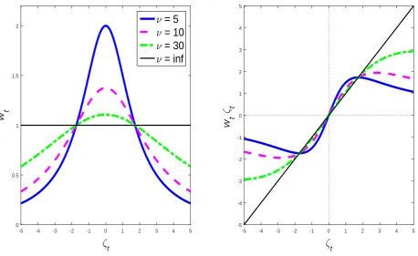
A crucial role in the score vector is played by the weights, wt, which are function of the

(squared) standardized prediction error, that is ζt =εt/σt. Figure 1 provides intuition for the

role played by those weights in the updating mechanism governing the model’s parameters.

The left panel plots the magnitude of wt as a function of the standardized prediction error,ζt.

Whereas the right panel plots the influence function (see e.g. Maronna et al. 2006), obtained

as the product of the weights and the standardized error itself. The magnitude of wt depends

on how close the observation yt is to the center of the distribution: a small value of wt is more

likely with low degrees of freedom and low dispersion of the distribution. The weightsrobustify

the updating mechanism because they downplay the effect of large (standardized) forecast

errors given that, in the presence of heavy tails, such forecast errors are not informative of changes in the location of the distribution. The right panel of Figure 1 shows how the score

is a bounded function of the prediction errors. Furthermore, the volatility, σt, plays a role in

re-weighting the observations, and as such the past estimated variance has a direct impact on

the coefficients’ updating rule.7 _{Therefore, the score vector (5)-(7) implies a double weighting}

scheme; i.e. the observation are weighted both over time and across realizations. [Insert Figure 1]

2.2

An example: the time-varying level model

A simplified version of model (1) helps clarify the impact of such double weighting

mech-anism. Assume that xt = 1 and wt is exogenously given. This specification leads to an

integrated moving-average (IMA(1,1), hereafter) model with TVP. In particular, the moving

average (MA) coefficient is equal to (1−κθwt), and the conditional mean can be expressed as

µt+1 =κθ t

X

j=0

γjy˜t−j, y˜t−j =wt−jyt−j, (8)

6_S−1

where

γj =

t

Y

k=t−j+1

(1−κθwk), γ0 = 1, κθ =κφ

(1−2η)(1 + 3η)

(1 +η) (9)

(see details in Appendix A). The observations are weighted to be robust to the impact of

extreme events through the weights wt, and simultaneously are discounted over time by γj.

Similarly, the time-varying variance can be expressed as

σ_t2₊₁ =κζ t

X

j=0

(1−κζ)jε˜2t−j, ε˜2t−j =wt−jε2t−j, (10)

where κζ =κσ(1 + 3η) regulates how past observations are discounted.8 In the presence of an

outlier (i.e. wt = 0), the MA coefficient collapses to one and the model becomes a pure random

walk.

In practice, the weights wt are not exogenously given but they depend non-linearly on the

current observation and the past estimated parameters through ζt = εt/σt. Therefore, under

the Student-t distribution the score-driven model leads to a non-linear filter that cannot be

analytically expressed as in the last two formulae. It is worth noticing that, since coefficients

and volatility are simultaneously updated, prediction errors of the same size are weighted

differently according to the conditional mean and volatility. Specifically, in periods of low

volatility, a given prediction error is more likely to be categorized as part of the tails and

therefore it is downweighted. This mechanism reinforces the smoothness of the filter in periods of low volatility. Conversely, the updating is quicker in periods of high volatility, with prediction

errors reflecting to a greater extent into parameters changes. As such, the weighting pattern is

non-monotonic and time-varying, and it cannot be easily replicated by the weighting schemes

which are meant to improve the forecasts under structural breaks, such as the ones proposed

by Pesaran et al. (2013) or Giraitis et al. (2014).

At this stage it is interesting to compare the filter implied by the our model to the one

of Stock and Watson (2007, SW hereafter). In particular, SW consider the local level model

with stochastic volatilities in both disturbances, this leads to a reduced form model equal to

an IMA(1,1) with TVP driven by a convolution of the two stochastic volatilities. In the SW model the MA coefficient drifts smoothly as a result of the random walk specification for the

stochastic volatilities, while in our score-driven model (with Student-t) the MA coefficient is

more volatile, because the time variation depends on the weights, wt, and the model discounts

the signal from the observations that are perceived as outliers.

8_{For larget we can interpret the estimated trend as the low-pass filterκ}

θ/[1−(1−κθwt)L] applied to the

weighted observations, ˜yt. Similarly, the estimated variance can be expressed by the filterκζ/[1−(1−κζ)L] applied to the weighted (squared) prediction errors, ˜ε2

2.3

The Gaussian case

The Gaussian case is recovered by setting η= 0 (i.e. υ → ∞). In this case wt = 1,∀t, and

the TVP are estimated by the following filter:

φt+1 = φt+κφ

1 σ2

t

S−1

t xtεt, (11)

σ2_t+1 = σ2_t +κσ(ε2t −σ

2

t). (12)

Equation (11) resembles the Kalman filter, since the updated parameters react to the

pre-diction error εt scaled by a gain, depending on σ2t and xt.9 Equation (12) is equal to the

integrated GARCH model. In contrast to the Student-t case, the volatility term vanishes in the law of motion of the coefficients, and the estimated conditional variance does not directly

affect the estimated time-varying coefficients.10

2.4

Estimation

Given the score vector (5)-(7) at time t, all the elements of the model (1)-(2) are known.

Hence, the conditional likelihood (4) can be analytically evaluated, and the log-likelihood

function is constructed asL(θ) =Pn

t=1`t, so that the vectorθis estimated asθb= arg maxL(θ).

Following Creal et al. (2013, sec. 2.3), we conjecture that √n(θb−θ) → N(0,Ω), where Ω is

numerically evaluated at the optimum.11

3

Model restrictions

Applications of TVP models often require imposing restrictions on the parameter’ space.

For instance, an AR model is usually restricted so that the implied roots lie within the unit

circle at each point in time. In the Bayesian framework, such constraints are usually imposed by

rejection sampling, which however leads to heavy inefficiencies (see e.g. Koop and Potter, 2011,

and Chan el al., 2013). When restrictions are implemented within a score-driven setup, the

model can still be estimated by ML without the need of computational demanding simulation

methods. Specifically, the TVP vector is reparametrized as follows

˜

ft=ψ(ft), (13)

9_{As opposed to standard parameter-driven models, both the signal and the parameters are driven by the}

prediction error. The model is therefore similar to the single source error model of Casalas et al. (2002) and Hyndman et al. (2008).

10_{Note that this feature is not shared by the equivalent parameter-driven models (see e.g. Stock, 2002).} 11_{Harvey (2013, sec 4.6) derives the consistency and asymptotic normality of a model with time-varying}

where ft is the unrestricted vector of parameters we model, while ˜ft, is the restricted vector

of interest with respect to which the likelihood function is expressed. The function ψ(·),

also known as link function, is assumed to be time-invariant, continuous, invertible and twice

differentiable. The vector ft continues to follow the updating rule (2), and the corresponding

score results in:

st= (Ψ0tStΨt)−1Ψ0tOt, (14)

where Ψt = ∂

˜

ft

∂ft0 is the Jacobian of ψ(·), while Ot and St are the gradient and the scaling

matrix expressed with respect to ˜ft. In practice, we modelft=h( ˜ft), whereh(·) is the inverse

function of ψ(·), and Ψt is needed to apply the chain rule when we compute the score. Given

past information, Ψt is a deterministic function whose role is to re-weight the score such that

the restrictions are satisfied at each point in time.

Specifically, for model (1) we have that ˜ft = (φ0,t, φ

0

t, σ

2

t)0, where φ_t = (φ1,t, ..., φp,t)0, and

ft = (α0,t, α0t, γt)0, where αt = (α1,t, ..., αp,t)0. The next sub-sections describe in detail how

to impose restrictions on the autoregressive coefficients φ_t and the intercept φ0,t, in order to

achieve local stationarity and bounded long-run mean of the process. The variance is always

constrained to be positive using the exponential function, σ2

t = exp(2γt), this implies that

γt= logσt. Given the the partition of ft and ˜ft, it is useful to specialize the Jacobian matrix

as follows:

Ψt=

   

∂φ0,t

∂α0,t

∂φ0,t

∂α0

t

∂φ

t

∂α0,t

∂φ

t

∂α0t

0

00 2σ2

t     , (15)

where ∂φ0,t

∂α0,t and 2σ

2

t are scalars,

∂φ0,t

∂α0

t and

∂φ_t

∂α0,t are 1×p and p×1 vectors respectively,

∂φ_t ∂α0

t is a

p×p matrix, and 00 is row vector of zeros.

3.1

Imposing local stationarity

The Durbin-Lenvinson (DL) algorithm maps the autoregressive coefficients (ARs) into the

partial autocorrelations (PACs). Local stationarity, which implies that at each point in time

the AR model has stable roots, is imposed by restricting the PACs within the unit circle.12

Notation 1 Given the vector of ARs φ

t = (φ1,t, ..., φp,t)

0 _{∈ R}p_{, z}

t = (z1,t, ..., zp,t)0 ∈ Cp

denotes the corresponding vector of roots, and ρt = (ρ1,t, ..., ρp,t)0 ∈ Rp is the corresponding

vector of PACs. Rp _{and C}p _{are the real and the complex domain respectively. Recall that}

α_t= (α1,t, ..., αp,t)0 ∈Rp is the unrestricted counterpart ofφ_t.

Definition 1 Model (1) is locally stationary if φ

t ∈S

p_{, ∀t, where S}p _{is the stationary}

hyper-plane where all the roots are inside the unit circle, i.e. |zj,t|<1, ∀t. Furthermore, φ_t ∈Sp if

and only if |ρj,t|<1, ∀t.

12_{Note that the logistic transformation considered by Blasques et al. (2014) is a special case of the general}

Definition 1 extends the results in Bandorff-Nielsen and Schou (1973) and Monahan (1984)

to the case of time-varying coefficients. For more details on locally stationary processes see

Dahlhaus (2012).

Assumption 1 Υ(·) is a continuous (invertible) and differentiable function mapping α_t∈Rp

into ρt∈Sp; i.e. ρj,t = Υ(αj,t), such that ρj,t <|1|, ∀t. Consequently, ∂Υ(_∂αα0t)

t =diag

h_∂Υ(α

j,t)

∂αj,t

i

.

In the application we use the Fisher transformation, i.e. Υ(αj,t) = tanhαj,t, this implies

that αj,t = arctanhρj,t, and

∂Υ(αj,t)

∂αj,t = (1−ρ

2

j,t).

Definition 2 Φ(·)is the continuous (invertible) and differentiable function mapping the PACs into the ARs, i.e. φ

t = Φ(ρt). Such function is obtained by the Durbin-Levinson (DL)

algo-rithm:

φ_ti,k =φi,k_t −1−ρk,tφtk−i,k−1, i= 1, ..., k−1, k = 2, ..., p, (16)

with φ1_t,1 =ρ1,t and φk,kt =ρk,t. For k=p we have that φj,t =φi,pt .

Corollary 1 Given Definitions 1-2, and Assumption 1, ψs(·) = Φ[Υ(·)]is the function

ensur-ing the model is the locally stationarity. Specifically, ψs(·) maps αt ∈ Rp into φ_t ∈ Sp; i.e.

φ

t=ψs(αt). The Jacobian of ψs(·) is equal to:

∂φ

t

∂α0

t

= ∂φt

∂ρ0

t

∂ρt

∂α0

t

⇒ ∂ψs(αt)

∂α0

t

= ∂Φ(ρt) ∂ρ0

t

∂Υ(α_t) ∂α0

t

. (17)

Theorem 1 Given Definition 2, the Jacobian ∂φt

∂ρ0

t =

∂Φ(ρt)

∂ρ0

t is equal to the last element of the

following recursion:

Γk,t=

"

˜

Γk−1,t bk−1,t

00_k−1 1

#

, Γ˜k−1,t =Jk−1,tΓk−1,t, k = 2, ..., p, (18)

where

bk−1,t =−

        

φk_t−1,k−1 φk_t−2,k−1

.. .

φ2_t,k−1 φ1_t,k−1

        

, Jk−1,t =

        

1 0 · · · 0 −ρk,t

0 1 0 −ρk,t 0

..

. . .. ...

0 −ρk,t 0 1 0

−ρk,t 0 · · · 0 1

         ,

φj,k_t −1 are the elements of (16), and fork even the central element ofJk−1,t is equal to(1−ρk,t).

The recursion is initialized with J1,t = (1−ρ2,t), and Γ1,t = 1.

Proof. See Appendix A.

Corollary 1 defines the link function through which we impose the stationarity restriction,

and Theorem 1 defines the Jacobian of function Φ(·) in Definition 2. When the time-varying

intercept φ0,t is included without restrictions, the remaining elements of the Jacobian matrix

(15) are: ∂φ0,t

∂α0,t = 1 and

∂φ0,t

∂α0

t =

_∂φ

t

∂α0,t

0

3.2

Bounded trend

Sometimes it may be the case that one wants to discipline the model so as to have a bounded

long-run mean (see e.g. Chan et al., 2013). Following Beveridge and Nelson (1981), a stochastic

trend can be expressed in terms of long-horizon forecasts. For a driftless random variable, the

Beveridge-Nelson trend is defined as the value to which the series is expected to converge once

the transitory component dies out (see e.g. Benati, 2007 and Cogley et al. 2010).

Definition 3 Given Definition 1, the local-to-date t approximation of the unconditional (time-varying) mean of model (1) is:

µt=

φ0,t

1−Pp

j=1φj,t

, ∀t. (19)

As a result, the detrended component, y˜t = (yt−µt), follows a locally stationary process, i.e.

Pr{limh→∞Et(˜yt+h) = 0}= 1.

Assumption 2 g(·)is a continuous (invertible) and differential function such thatg(·)∈[b, b].

In the application we use g(α0,t, b, b) =

b+bexpα0,t

1+expα0,t . This implies that α0,t = log

µt−b

b−µt

and

∂g(α0,t,b,b)

∂α0,t =

(b−b) expα0,t

(1+expα0,t)2.

Corollary 2 Given Definition 3 and Assumption 2, ψb(·) is the function mapping the

unre-stricted intercept α0,t (and the restricted φ_t) into its restricted counterpart φ0,t, in order to have

µt∈[b, b]; i.e. φ0,t =ψb

α0,t, b, b, φ_t

. Specifically,

ψb(·) =g α0,t, b, b

1− p X j=1 φj,t ! . (20)

Given ψb(·), the elements of the Jacobian matrix (15) are equal to:

∂φ0,t

∂α0,t

= ∂g α0,t, b, b

∂α0,t

1− p X j=1 φj,t !

, ∂φ0,t

∂α0

t

=−g α0,t, b, b

ι0∂φt ∂α0

t

, ∂φt

∂α0,t

= 0, (21)

where ι0 is a p-dimensional row vector of ones, 0 is a p-dimensional column vector of zeros, and ∂φt

∂α0_t has been outlined in Corollary 1.

Corollary 2 defines the link function, and the corresponding Jacobian, through which the

bounds on the long-run mean are imposed. Putting together (17) and (21), we have all the

elements of the Jacobian matrix (15).

4

Application: inflation forecasting

Autoregressive models have been shown to work well in the context of forecasting inflation

following features of inflation dynamics: (i) substantial time variation in trend inflation (e.g.

Cogley, 2002, and Stock and Watson, 2006); (ii) changes in persistence (Cogley and Sargent,

2002, and Pivetta and Reis, 2007); (iii) time-varying volatility (e.g. Stock and Watson, 2007,

and Clark and Doh, 2014).

In this section we use the score-driven model introduced in Section 2 to capture the key

characteristics of inflation dynamics. In particular, we emphasize the importance of allowing

for t-distributed innovations to the TVP autoregressive specification:

πt=φ0,t+ p

X

j=1

φj,tπt−j+εt, εt∼tυ(0, σ2t), (22)

where πt in the annualized quarterly inflation.13 Various specifications of model (22) are

con-sidered in terms of lags (p= 0,1,2,4) and restrictions. The model is reparameterized so that

the variance is positive and, for p >0,the model is locally stationary as shown in sub-section

3.1. For each specification, we also consider a counterpart with bounds on the long-run trend,

as shown in sub-section 3.2. The choice of the bounds (between 0 and 5) follows the work by

Chan et al. (2013), who argue that a level of the trend inflation that is too low (or too high) is

inconsistent with the central bank’s inflation target.14 Finally, for all specifications we consider

both Gaussian and Student-t distribution of the innovations.

For the case with p = 0, we have a time-varying level that tracks trend inflation. In

particular, with Gaussian innovations trend inflation is estimated by exponential smoothing,

as in Cogley (2002).15

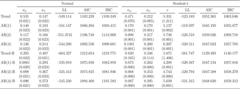
[Insert Table 1]

Table 1 reports the estimates of the various specifications for CPI inflation in the US,

over the period 1955Q1–2012Q4. Besides the estimates of the parameters and their associated

standard error, we also report the value of the log-likelihood function, the Akaike (AIC) and the Bayesian Information Criterion (BIC).

The trend-only specification (p = 0) features a high estimated value of the smoothing

parameter κφ, implying that past observations are discounted more heavily. This is also true

for the specification with Student-t distribution. By adding the autoregressive component

we obtain substantially smaller estimates of κφ, and this is due to the fact that part of the

persistence of inflation is captured by the autoregressive terms. By contrast, the smoothing

parameter associated with the variance, κσ, is stable and typically higher than κφ. This

13_{The bulk of the analysis focuses on US CPI inflation. Section 4.3 shows that the superiority of the model}

with Student-t distributed errors (in terms of forecasting) carries over different indicators of US inflation (PCE and GDP deflators), as well as for the CPI inflation of the remaining G7 countries. The data sources are discussed in Appendix B.

14_{The bounds correspond to the upper and lower bounds of the posterior in Chan et al. (2013).}

15_{Notice that Cogley (2002) does not include time variation in the variance. However, as it has been shown}

result supports the idea that changes in the volatility are an important feature of inflation

(see e.g. Pivetta and Reis, 2007). Noticeably, the specifications with Student-t distribution

considerably outperform the ones with Gaussian innovations, both in terms of the likelihood

values and information criteria. The estimates of the degrees of freedom υ, between 4 and

6, depict a remarkable difference between the Gaussian and the Student-t specification and

underline the presence of pronounced variations of inflation at the quarterly frequency. Those

variations either arise from measurement errors or are due to the presence of rare events that

structural macroeconomics should explicitly account for, as recently advocated by C´urdia et

al., 2014. Notice that υ = 5 is also consistent with the calibrated density forecast in Corradi

and Swanson (2006). Overall, the AR(1) model without bounds on the long-run mean and

Student-t distribution slightly outperforms all the other specifications in terms of fitting.

4.1

Trend inflation and volatility

In this sub-section we show that our model is able to capture the salient features of

infla-tion dynamics in terms of trend inflainfla-tion and volatility. Furthermore, we highlight the main

differences between the specifications with Gaussian and Student-t distribution.

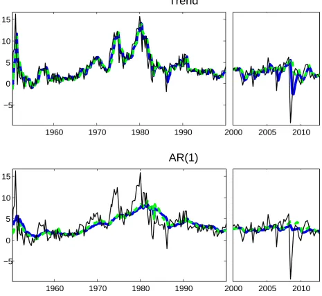
Figure 2 compares the estimates of the long-run trend for the trend-only and the AR(1)

specifications.16 _{The trend-only specification tracks inflation very closely through the ups}

and downs, whereas including lags of inflation leads to a smoother long-run trend estimate.

Therefore, when we allow for intrinsic persistence a substantial part of inflation fluctuations

during the high inflation period (i.e., in the early part of the sample and in the 70s) is attributed

to deviations from the trend. For all specifications we find that, since the mid 90s, the long-run

trend is stable between 2-3%, going slightly over 3% in the run up to the recent recession.

Focussing on differences between the models with Gaussian and Student-t innovations, one

notes that the trend-only model with Student-t innovations is generally less affected by the sharp transitory movements in the underlying inflation rates. In fact, the updating mechanism

for the TVP under Student-t innovations is such that the observation is downplayed when it

is perceived as an outlier. These differences are most visible in the last part of the sample,

where the underlying trend inflation from the model with Gaussian innovations is often revised

after large, but one-off, releases of inflation.17 _{Once lagged inflation is included, the differences}

between the two specifications are attenuated, both of them deliver a very smooth outline of

trend inflation but some differences are apparent in the last part of the sample. In this latter

case, the outliers still have an impact on the parameters’ estimates for the Gaussian model,

whereas they have a smaller effect under a Student-t distribution. However, the variation in the time-varying intercept is offset by the variation in the autoregressive coefficients, and the

16_{Adding more lags has very little impact on the estimates of long-run mean (see Appendix D). Therefore,}

the choice of the lag length has an impact only on the shape of the dynamics toward the long-run level, i.e. on short to medium horizon forecasts.

17_{Aastveit et. al (2014) have recently reported evidence of instability in standard VARs since the financial}

model ends up delivering rather smooth long-run forecasts.18

Imposing an upper bound on the long-run mean implies a qualitatively similar picture for

the trend-inflation across all specifications (see Appendix D). In this case the trend estimates

are consistent with the idea of a central bank anchoring expectations of trend-inflation to a fairly stable level over the sample. Trend-inflation rises above 3% in the early ’70s and then

decreases back to a slightly lower level only in the mid ’90s.19

[Insert Figure 2]

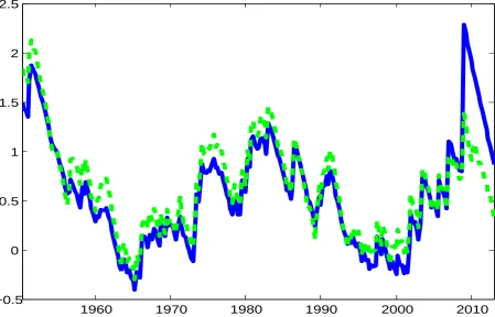
Figure 3 reports measures of changes in volatility for the AR(1) specification with

Gaus-sian and Student-t innovations.20 _{For both specifications it is true that the variance was}

substantially higher in the 50s, in the 70s and then again in the last decade. This pattern

of the volatility is consistent with Chan et al. (2013) and Cogley and Sargent (2015). Yet,

there are some interesting differences between the two models. First, the model based on the Student-t distribution is more robust to single outliers; under Gaussian distribution the

volatility seems to be disproportionately affected by very few observations in the last part of

the sample.21 _{Second, although the volatility shows very similar low-frequency variation across}

different specifications, under Student-t the model displays substantially more high-frequency

movements in the volatility. Note also that under Student-t the observations are weighted such

that large deviations are heavily down-weighted and small deviations are instead magnified.

In other words, under Student-t the variance is less affected by the outliers and it can better

adjust to accommodate changes in the dispersion of the central part of the distribution. The

latter result is particularly important in light of the superior in sample fit of the Student-t spec-ification reported in the previous sub-section. It is worth noting that most of the literature,

which has mainly focused on the Gaussian distribution, has only reported and emphasized the

importance of the low frequency variation in the volatility.

[Insert Figure 3]

18_{In order to clarify this point it is instructive to look at what happens to the autoregressive coefficients}

in the Gaussian model in response to the inflation shift in 2008. The 2008:Q3 observation (approximately -9%) is clearly a tail event given the usual inflation variability. This single observation leads to a shift of the autoregressive coefficient from approx. 0.8 to -0.5. At the same time, the shift in the long-run trend is slightly less than 1%, as a result of a simultaneous jump in the intercept. Conversely, the long-run trend under Student-t barely varies as a result of the same episode.

19_{It is worth noting that the pattern in the long-run trend is quite similar to the one found by Chan et al.}

(2013), despite the fact that they use a different model specification and different estimation techniques.

20_{Small differences can be appreciated when comparing the trend-only model to the AR(p) specifications}

(see Appendix D).

21_{Again, it is worth to report what happens as a result of a single tail event in 2008:Q3: the log-volatility}

4.2

Forecast evaluation

In this section we assess the forecasting performance of the model. The various

specifica-tion are evaluated against the SW model that is usually considered to be a good benchmark

for inflation forecasting.22 _{The models are estimated recursively, over an expanding window.}

Consistent with a long standing tradition in the learning literature (referred to as

anticipated-utility by Kreps, 1998), we update the coefficients period by period and we treat the updated

values as if they remained constant going forward in the forecast. We first assess the point

forecast using both the root mean squared error (RMSE) and the absolute mean error (MAE).

Later on, we will evaluate the performance of the models in terms of their density forecasts.

4.2.1 Point Forecast

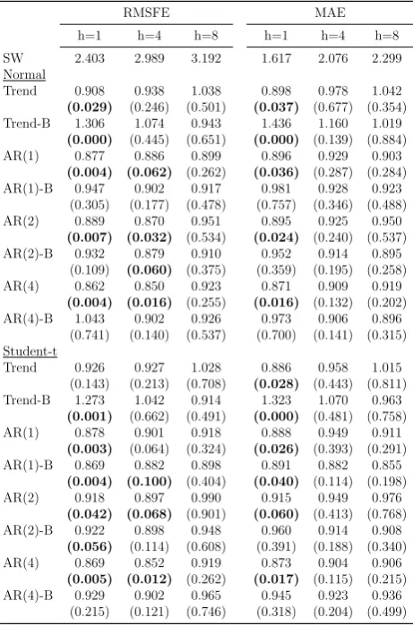
Table 2 reports the results for the point forecast. Despite the well-known performance of the

benchmark model, many of the alternative specifications we consider tend to have lower RMSEs

and MAEs. The differences tend to disappear at longer horizons. The superior forecasting

performance is also statistically significant for many specifications.23 For instance, the AR(4)

model reduces the loss by roughly 15%, both for the one quarter and one year ahead forecast.

Imposing bounds on the long-run mean does not seem to improve the performance of the

various specifications.24 _{Most importantly, a comparison between the Gaussian and Student-t}

models reveals little differences in terms of point forecasts.

[Insert Table 2]

Looking at the relative performance in different sub-samples reveals that the score-driven

models are superior at the beginning and at the end of sample, while the SW model is slightly

better in the low volatile period (from mid-80s to early 2000). None of these differences are

significant using the fluctuation tests of Giacomini and Rossi (2010), highlighting a relatively high volatility of the forecast errors.

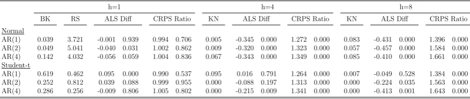
4.2.2 Density Forecast

An important element of any forecast lies in the ability to quantify and convey the

out-come’s uncertainty. This requires a forecast of the whole density of inflation. For instance,

Cogley and Sargent (2015) highlight the relevance of deflation risk, and the prediction of

the latter requires an estimation of the overall density. Table 3 reports the results from the

22_{The SW model is estimated by Bayesian MCMC methods, and the Gibbs Sampling algorithm is broken}

into the following steps: (i) sampling of the variance of the noise component using the independent Metropolis Hastings as in Jacquier et al. (2002); (ii) sampling of the variance of trend component as in (i); (iii) sampling of the trend component using the algorithm developed by Carter and Kohn (1994).

23_{We report the test of Giacomini and White (2006). Despite the expanding window, this test is}

approx-imately valid as our model implicitly discount the observations, so that earlier observations are in practice discarded for the estimates in the late part of the sample that is used to forecast.

24_{The trend-only model with restricted long-run mean is outperformed by the alternative ones, in particular}

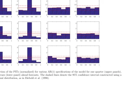
density forecast exercise. As highlighted by Diebold et al. (1998), a correctly conditionally

calibrated density forecast produces probability integral transforms (PITs) that are uniformly

distributed.25 For the one step-ahead we evaluate the calibration of the densities looking at

the results of Berkowitz’s (2001) LR test and the nonparametric test of Rossi and Sekhposyan

(2014).26 _{For horizons beyond the one step-ahead we report the test of Kn¨uppel (2015), which}

is robust to the presence of serial correlation of the PITs. The results suggest that, at all

hori-zons, the density forecasts of specifications with Gaussian innovations, as well as for the SW

model, are not well calibrated. In order to understand why this is the case Figure 4 plots the

empirical distribution function (p.d.f.) of the PITs for the AR(1) specification.27 _{From both}

plots it is evident that models with Gaussian innovations tend to produce densities in which

too many realizations fall in the middle of the distribution relative to what we would expect

if the data really were Normally distributed.28 The one step-ahead density forecasts are well

calibrated for all the specifications with Student-t distribution. Two key features are important to deliver correctly calibrated forecasts. First, the volatility is not affected by observations in

the tail of distribution, thus varying in a way that better captures changes in the dispersion of

the central part of the density. Second, the distribution by nature has a slower decay in the

tail. As such, it allows for higher probability of extreme events. According to Kn¨uppel’s (2015)

test, the multistep density forecasts are well calibrated when we allow for Student-t innovations

and also we impose bounds to the long-run mean. This restriction effectively imposes a tight

anchor to far ahead forecasts, which turns out to be important in order to avoid that too many

realizations fall in the tails of the distribution.

[Insert Table 3]

[Insert Figure 4]

Table 3 reports measures of the relative performance of density forecasts for various models,

evaluating the relative improvements with respect to the SW model. The average logarithm score (ALS) suggests that the models with Student-t distribution significantly improve the

accuracy of the density forecast and outperform considerably both the SW benchmark as well

as all the specifications with Gaussian errors at all forecasting horizons. We also evaluate

density forecasts looking at the average Continuous Ranked Probability Score (CRPS). The

latter provides a metric for the evaluation of the density that is more resilient in the presence

of outliers (Gneiting and Ranjan, 2007). The models under Student-t innovation continue to

dominate the SW benchmark. Yet, since the CRPS is less sensitive to the realizations falling

at the tails of the forecast density, the performance from the Student-t model are roughly in

25_{The PITs are also iid for one step ahead forecasts.}

26_{The latter is still valid also in the presence of parameter estimation errors.}

27_{Appendix D reports a similar plot for the other specifications. These figures confirms that only the PITs}

of the densities from the adaptive models with Student-t innovations resemble a uniform distribution.

28_{The histogram of the PITs for the SW model is similar to the one obtained for the score-driven models}

line with the ones produced by the model under Gaussian innovations under this alternative

scoring metric. The model with Student-t innovations provides a better characterization of the

density at the tail of the distribution. This superiority is clearly highlighted when looking at

the ALS.29

4.2.3 Robustness

Forecasting performance over time. It is possible that the superiority of the heavy tail

specification is not stable over the entire forecasting sample. For instance, the robustness of

the model under a Student-t distribution can potentially delay the updating of the parameters

in presence of a marked, isolated, structural break. In this case, a Gaussian model adapts more

quickly to the new regime, while the Student-t model initially downweighs the observations occurring after the break. In order to understand whether the improvements under

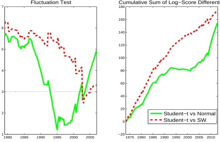
Student-t are driven by parStudent-ticular episodes, or specific sample periods, as opposed Student-to be sStudent-table over

time, Figure 5 reports: (a) the fluctuation test of Giacomini and Rossi (2010) applied to

the ALS (left panel), and (b) the cumulative sum of the log-score (CLS) over time (right

panel). We consider the trend-only specification with Student-t versus the Gaussian case and

the SW model, focussing on the one quarter ahead forecast.30 _{The value of the Giacomini}

and Rossi (2010) statistics is always positive and the CLS is rising. This suggests that the

densities produced by the heavy tails model deliver a consistently higher log-score throughout

the sample. The differences between Gaussian and Student-t innovations are, however, not statistically significant in the 90s and the CLS shows a slight decline over this period. This is

not surprising since in the 90s inflation has been quite stable and as such we would not expect

considerably different densities produced by the two models.

[Insert Figure 5]

Evaluating the importance of local stationarity restrictions. In the empirical

anal-ysis we have always imposed local stationarity, as a result inflation forecasts are forced to

revert to the time-varying long-run mean. Instead, when local stationarity restrictions are not

enforced, forecasts are in principle allowed to diverge over time. Although one can justify the imposition of stationarity restrictions on theoretical grounds, a natural question to ask is how

relevant those restrictions are in practice. Table 4 highlights that the density forecasts produced

without imposing stationarity restrictions are roughly in line with the restricted counterpart

only for short-run forecast, i.e. one quarter ahead. However, at the 1 and 2 years horizon the

density forecasts produced by a model that does not impose stationarity restrictions delivers

29_{The adaptive model developed in this paper delivers a model-consistent way to deal with time-variation in}

presence of heavy tailed distribution. Appendix C explores the importance of using an updating mechanism for the parameters, which is consistent with the score-driven approach as opposed to some ad-hoc specifications. Specifically, allowing for low degrees of freedom as well as for an updating mechanism that downplays the importance of outliers are both important ingredients to achieve well calibrated density forecasts.

30_{The results are qualitatively similar when other autoregressive specifications and longer forecast horizons}

significantly worse ALS and CRPS than the restricted counterpart.31

[Insert Table 4]

4.2.4 Comparison with a TVP-VAR with stochastic volatility

In this section we compare the forecasting performance of our adaptive model with that

of an alternative benchmark, the TVP-VAR with stochastic volatility. This model is often considered the state of the art technology when it comes to modelling macroeconomic time

series facing structural changes. In particular, D’Agostino et al. (2013) have highlighted that

the TVP-VAR produces forecasts that are superior to a number of alternative specifications

(both with fixed coefficients and more parsimonious specifications with TVP). Barnett et al.

(2014) highlight that TVP-VAR leads to large improvements in forecast of UK macroeconomic

time series. Clark and Ravazzolo (2015) compare different volatility specifications, including

specifications with fat tails, and conclude that none dominates the standard stochastic volatility

specification considered as a benchmark in this section.

We consider a VAR with 2 lags and three variables: unemployment, the short term interest

rate, and inflation.32,33 _{The TVP-VAR produces long-run forecasts that are potentially more}

precise than the one produced by a univariate model. In fact, the multivariate setting allows the

TVP-VAR to exploit the information contained in the level of unemployment and the interest

rate in predicting long-run inflation and the associated uncertainty around the forecast. In order

to check for that in this section we consider forecasts of inflation up to 4 years ahead. In order

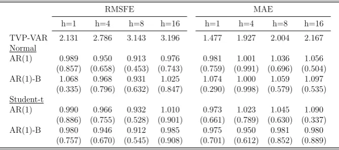
to save space we focus on a comparison with the AR(1) specification of the adaptive model.

The adaptive model specifications and the TVP-VAR produce very similar point forecasts (see

Table 5). Whereas the Student-t specifications are typically marginally better both in terms

of RMSE and MAE, the difference with respect to the forecasts produced by the TVP-VAR

are never statistically significant according to the Giacomini and White (2006) test.34

[Insert Table 5]

Table 6 turns to the comparison of the models in terms of density forecast. Density

fore-casts produced by the TVP-VAR are well calibrated at the short horizons but fail to correctly

31_{The densities for the one quarter ahead are correctly calibrated only for the models with Student-t}

inno-vations. At longer forecast horizons are typically not correctly calibrated.

32_{The choice of variables and lag order is in line with the literature (e.g. Primiceri, 2005, and D’Agostino et}

al., 2013). The results with a single lag are qualitatively in line with the ones reported in this section and are available from the authors upon request.

33_{The TVP-VAR model with stochastic volatility model is estimated by Bayesian MCMC methods. The}

Gibbs Sampling algorithm is broken into the following steps: (i) sampling of the time varying coefficients of the VARs using the algorithm developed by Carter and Kohn (1994); (ii) sampling of the diagonal elements of the VAR covariance matrix model using the Metropolis Hastings as in Jacquier et al. (2002); (iii) sampling of the off-diagonal elements of the VAR covariance matrix using the algorithm developed by Carter and Kohn (1994). The priors of the model are chosen as in Cogley and Sargent (2005).

34_{Table D.1 in Appendix D reports that there is no statistically significant difference in point forecasts for}

characterize the distribution of inflation for longer horizons.35 _{Moreover, the TVP-VAR}

pro-duces CRPS which are broadly in line with the one produced by the adaptive AR(1) model.

However, there are large differences in terms of average log-score (ALS). The ALS associated

with the density produced by the TVP-VAR model is almost always superior to the one pro-duced by the specification of the model with Gaussian innovations, but it is substantially lower

than most specifications which allow for heavy tails. Those differences are large and always

statistically significant according to the Amisano and Giacomini (2007) test. These results

hold at all forecasting horizons, including forecasts of inflation 4 years ahead.36

[Insert Table 6]

[Insert Figure 6]

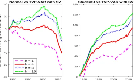
Figure 6 reports the cumulative logarithm score of the models for different forecasting

horizons of the AR(1) specification against the TVP-VAR. The log-score differences between

the adaptive model with heavy tail and the TVP-VAR are almost always positive for forecasts

horizons longer than one quarter. For short-run forecasts there are two periods, in the late

70s and the mid-90s, when the TVP-VAR produces higher log-scores. The gains in these two

periods are however overshadowed by the superior performance of the adaptive heavy tail model for the remaining part of the sample. The differences between the two models seem to be larger

in the last decade of the sample, with inflation showing a more volatile and erratic behaviour.

Overall, the gains in terms of log-score are larger for more distant horizons. Summarizing, in

this comparison a clear ranking emerges: when forecasting inflation the adaptive AR model

with Gaussian errors is dominated by a state-of-the art multivariate TVP benchmark but the

adaptive model with heavy tails proves to be superior in density forecast to both approaches.

Although our univariate model does not allow us to generalize this conclusion to other variables,

it strongly points to potential advantages in combining heavy tails with TVP.

4.3

Additional empirical evidences

4.3.1 Alternative inflation indicators

In the previous section we have shown how the model with Student-t errors produces time

variation in the parameters which is robust to the presence of heavy tails. Furthermore, the

volatility is less affected by the behavior in the tail of the distribution, so that it can better

reflect changes in the spread of the central part of the density. These aspects of the model are

key in order to retrieve a well calibrated density forecasts of US CPI inflation. However, CPI

35_{Figure D.10 in Appendix D shows the PITs associated to the forecast and highlights that the long-horizons}

forecasts of TVP-VAR tend to be too wide so that far too many of the inflation turnout are scored in the middle part of the distribution.

36_{Comparing the results in Table 6 to the ones in Table 3, we note that the forecasts from the TVP-VAR}

inflation is notoriously more volatile than other inflation indicators, such as the PCE deflator

and GDP deflator.37 In order to assess whether the improvements of the heavy tails model

carry through for other measures of inflation, we repeat the forecasting exercise using these two

additional measures of inflation. The results we obtain are in line with the evidence reported in the previous section. To preserve space we focus on the density forecast while the results for

the point forecast are reported in Appendix D.38_{Table 7 shows that for these two indicators the}

one quarter ahead densities forecast are well calibrated only under the Student-t specifications.

For 1 and 2 years ahead forecast most of the specifications tend to be poorly calibrated. An

inspection of the PITs reveals that the problems are less severe when we allow for the Student-t

distribution. Moreover, the models under Student-t tend to outperform the SW benchmark, as

well as all the Gaussian specifications, and by a considerable margin, when looking at the ALS.

The CRPS tend to be similar between the Gaussian and Student-t specifications and, in all

cases, are lower than the SW benchmark. Interestingly, since those two indicators are smoother than CPI inflation, adding lags of inflation can in some cases deliver significant improvements

in the density forecast.

[Insert Table 7]

4.3.2 International evidence

Cecchetti et al. (2007) highlight the presence of similarities in inflation dynamics across

countries. Therefore, we investigate the performance of our model for CPI inflation of the

remaining G7 countries. Table 8 reports a summary of the density evaluation focussing on the

trend-only model.39 The results are in line with those reported for the US. Specifically, the

model with heavy tails results in large gains in terms of ALS and similar CRPS. Moreover, for

one quarter ahead forecasts the densities are well calibrated only when the Student-t

distri-bution is allowed. At longer horizons most specifications tend to be not well calibrated. An

inspection of the PITs reveals that the problems are more severe for the model with Normal

innovations.

[Insert Table 8]

5

Conclusion

In this paper we derive an adaptive algorithm for time-varying autoregressive models in

presence of heavy tails. Following Creal et al. (2013) and Harvey (2013), the score of the

37_{SW report that their model is better suited for those smoothed series.}

38_{The point forecast assessment confirms that various specifications outperform, on average, the SW model.}

However, the differences are statistically significant only for few specifications and mainly for short forecast horizons.

39_{For the remaining G7 countries the trend-only model with Gaussian distribution is the benchmark}

conditional distribution is the driving process for the evolution of the parameters. In this

context, we emphasize the importance of allowing for time variation in both parameters and

volatilities. In the presence of Student-t innovations the updating mechanism for the TVP

downplays the signal when the observation is perceived to be in the tail of the distribution. A given prediction error is more likely to be categorized as part of the tails in periods of

low volatility than in periods of high volatility. Furthermore, the algorithm is extended to

incorporate restrictions which are popular in the empirical literature. Specifically, the model is

allowed to have a bounded long-run mean and the coefficients are restricted so that the model

is locally stationary. The model introduced in this paper does not require the use of simulation

techniques. As such, it entails a clear computational advantage, especially when restrictions

on the parameters are imposed.

We apply the algorithm to the study of inflation dynamics. Several alternative specifications

are shown to track the data very well, so that they give a parsimonious characterization of inflation dynamics. The specifications with Student-t innovations are more robust to short

lived variations in inflation, especially in the last decade. Furthermore, the use of heavy-tails

highlights the presence of high-frequency variations in volatility on top of well documented

low-frequency variations.

The proposed model produces forecasts that are comparable in terms of point forecasts and

far superior in terms of density forecasts than the model of Stock and Watson (2007) and a

TVP-VAR with stochastic volatility. Allowing for heavy tails is found to be a key ingredient

to obtain well calibrated density forecasts; only in this case one has a correct characterization

of the density at the tail of the distribution. Imposing restrictions to the TVP of the model is relevant in order to produce better forecasts. For long-run horizons, imposing local stationarity

improves substantially the performance in terms of density forecasts. Moreover, imposing the

bounds on the long-run mean of the model improves the density forecasts for 1 and 2 years

ahead.

The results of this paper can be extended along various directions. Whereas the empirical

analysis is centered around the study of inflation dynamics we suspects that similar gains in

forecasting performance extend to other macroeconomic time series. Furthermore, the model

can be extended (along the lines of Koop and Korobilis, 2013) to the multivariate case, where

the dimensions of the model might be so large that the use of computationally intensive

References

Aastveit, K., A. Carriero, T. Clark and M. Marcellino (2014). Have Standard VARs Remained Stable Since the Crisis? Cleveland Fed Working paper 14-11.

Amisano, G. and R. Giacomini (2007). Comparing Density Forecasts via Weighted Likelihood Ratio Tests. Journal of Business and Economic Statistics, 25, 177-190.

Bandorff-Nielsen, O. and G. Shou (1973). On the Parametrization of Autoregressive Models by Partial Autocorrelations. Journal of Multivariate Analysis, 3, 408-419.

Barnett, A., Haroon, M. and K. Theodoridis (2014). Forecasting UK GDP growth and in-flation under structural change. A comparison of models with time-varying parameters. International Journal of Forecasting, vol. 30(1), 129-143.

Benati, L. (2007). Drift and breaks in labor productivity, Journal of Economic Dynamics and Control, 31(8), 2847-2877.

Berkowitz, J. (2001). Testing Density Forecasts with Applications to Risk Management.

Journal of Business and Economic Statistics, 19, 465-474.

Beveridge, S. and C.R. Nelson (1981). A new approach to decomposition of economic time se-ries into permanent and transitory components with particular attention to measurement of the business cycle. Journal of Monetary Economics, 7, 151-174.

Blasques F., Koopman S.J. and A. Lucas (2014). Optimal Formulations for Nonlinear Au-toregressive Processes. Tinbergen Institute Discussion Papers TI 2014-103/III.

Bollerslev, T. (1987). A Conditionally Heteroskedastic Time Series Model for Speculative Prices and Rates of Return. Review of Economics and Statistics, 69, 542-547.

Carter, C. K. and Kohn, R. (1994). On Gibbs Sampling for State Space Models. Biometrika, 81(3), 541-553.

Casales, J., Jerez, M. and S. Sotoca (2002). An Exact Multivariate Model-Based Structural Decomposition. Journal of the American Statistical Association, 97, 553-564.

Cecchetti, S. G., Hooper, P., Kasman, B. C., Schoenholtz, K. L. and M.W. Watson (2007). Understanding the Evolving Inflation Process. U.S. Monetary Policy Forum 2007.

Chan, J.C.C., Koop, G. and S.M. Potter (2013). A New Model of Trend Inflation. Journal of Business and Economic Statistics, 31(1), 94-106.

Clark, T.E. and T. Doh (2014). A Bayesian Evaluation of Alternative Models of Trend

Inflation. International Journal of Forecasting, vol. 30(3), 426-448.

Clark, T. E. and F. Ravazzolo (2015). The macroeconomic forecasting performance of au-toregressive models with alternative specifications of time-varying volatility. Journal of Applied Econometrics, 30(4), 551-575.

Cogley, T. (2002). A Simple Adaptive Measure of Core Inflation. Journal of Money, Credit and Banking, 34(1), 94-113.

Cogley, T. and T.J. Sargent (2005). Drifts and Volatilities: Monetary Policies and Outcomes in the Post WWII US. Review of Economic Dynamics, 8(2), 262-302.

Cogley, T. and T.J. Sargent (2015). Measuring Price-Level Uncertainty and Instability in the U.S., 1850-2012. Review of Economics and Statistics, 97(4), 827838.

Cogley, T., Primiceri, G. and T.J. Sargent (2010). Inflation-Gap persistence in the US.

American Economic Journal: Macroeconomics, 2(1), 43-69.

Cooley, T. F. and E.C. Prescott (1973). An Adaptive Regression Model. International Eco-nomic Review, 14(2), 364-71.

Cooley, T. F. and E.C. Prescott (1976). Estimation in the Presence of Stochastic Parameter Variation. Econometrica, 44(1), 167-84.

Corradi, V. and N.R. Swanson (2006). Predictive Density and Conditional Confidence Interval Accuracy Tests. Journal of Econometrics, 135, (1-2),187-228.

Creal, D., Kopman, S.J. and A. Lucas (2013). Generalised Autoregressive Score Models with Applications. Journal of Applied Econometrics, 28, 777-795.

C´urdia, V., Del Negro, M. and D.L. Greenwald (2014). Rare shocks, Great Recessions.

Jour-nal of Applied Econometrics, 29, 1031-1052.

D’Agostino, A., Gambetti, L. and D. Giannone (2013). Macroeconomic forecasting and struc-tural change. Journal of Applied Econometrics, 28(1), 82-101.

Dahlhaus, R. (2012). Locally stationary processes. Handbook of Statistics, 30.

Diebold, F.X , Gunther, T.A. and S.A. Tay (1998). Evaluating Density Forecasts with Appli-cations to Financial Risk Management. International Economic Review, 39(4), 863-83.

Engle, , R. F. (1982). Autoregressive Conditional Heteroscedasticity with Estimates of the Variance of United Kingdom Inflation. Econometrica, 50(4), 987-1007.

Evans, G.W. and S. Honkapohja (2001). Learning and Expectations in Macroeconomics. Princeton University Press.

Faust, J. and J.H Wright (2013). Forecasting Inflation. Handbook of Economic Forecasting, Vol 2A, Elliott G. and A. Timmermann Eds. North Holland.

Fiorentini, G., Sentana, E. and G. Calzolari (2003). Maximum Likelihood Estimation and Inference in Multivariate Conditionally Heteroskedastic Dynamic Regression Models with Student t Innovations. Journal of Business and Economic Statistics, 21(4), 532-546.

Giraitis, L., Kapetanios, G. and T. Yates (2014). Inference on stochastic time-varying coeffi-cient models. Journal of Econometrics, 179(1), 46-65.

Giacomini, R. and B. Rossi (2010). Forecast comparisons in unstable environments. Journal of Applied Econometrics, 25(4), 595-620.

Giacomini, R. and H. White (2006). Tests of Conditional Predictive Ability. Econometrica, 74(6), 1545-1578.