Volatility and correlation in financial markets: Econometric modeling and empirical pricing

The London School of Economics and Political Science

Volatility and Correlation

in Financial

Markets:

Econometric Modeling and Empirical Pricing

Runquan Chen

A thesis submitted to the Department of Finance of the

London School of Economics for the degree of Doctor of

Finance

UMI Number: U615B0B

All rights reserved

INFORMATION TO ALL USERS

The quality of this reproduction is dependent upon the quality of the copy submitted.

In the unlikely event that the author did not send a complete manuscript and there are missing pages, these will be noted. Also, if material had to be removed,

a note will indicate the deletion.

Dissertation Publishing

UMI U615303

Published by ProQuest LLC 2014. Copyright in the Dissertation held by the Author. Microform Edition © ProQuest LLC.

All rights reserved. This work is protected against unauthorized copying under Title 17, United States Code.

ProQuest LLC

Declaration

I certify that the thesis I have presented for examination for the MPhil/PhD degree o f the London School o f Economics and Political Science is solely my own work other than where I have clearly indicated that it is the work o f others (in which case the extent o f any work carried out jointly by me and any other person is clearly identified in it).

The copyright o f this thesis rests with the author. Quotation from it is permitted, provided that full acknowledgement is made. This thesis may not be reproduced without the prior written consent o f the author.

Abstract

This thesis is an empirical study o f the volatility and correlation in financial markets, and consists

o f two parts: The first part is on econometric modeling o f the volatility and correlation (Chapter 1).

The second part is on the pricing implication o f the correlation and volatility as risk factors

(Chapter 2 and 3). The thesis begins with proposing a regime-switching multivariate GARCH

model o f volatilities and correlation. We incorporate the Markov-switching mechanism into the

Constant Conditional Correlation model (CCC). The proposed model allows us to capture the

different dynamics in both the volatilities and correlations in different regimes. It is particularly

useful in examining the contemporaneous relationship between the unobservable volatility and

correlation processes. We apply our model to the stock market index paired with two bond market

indexes.

Then in the second chapter, we estimate the risk premium for the average correlation in the

cross-section o f the US stock market. The average correlation is the cross-sectional average o f the

correlations between each pair o f stocks in the stock market. We find there is a negative and

statistically significant risk premium for the average correlation controlling for other factors such

as Fama-French’s SMB and HML as well as the liquidity factor and momentum factor.

The third chapter focuses on the risk-retum relation using a set o f variance-related risk

measures. We combine two lines o f literature both o f which find significant forecasting power o f

some risk measures for stock market returns: variance risk premium literature and studies on

average variance-correlation decomposition .We illustrate how these two approaches can be

Acknowledgements

Contents

Introduction

p age 1

Chapter 1

page 4

Topic: Regime Switching in Volatilities and Correlation between Stock and Bond markets

Chapter2

p a g e 52

Topic: Correlation Risk and Expected Equity Returns

Chapter 3

p age 84

Introduction

The market risk o f financial assets is generally measured by the second moment o f their returns. For

a portfolio with multiple assets, its risk is jointly determined by the variances o f individual assets

and the correlations between each pair o f assets. For an investor with a typical risk-averse utility, he

will optimize his asset holdings taking into account o f the correlations and variances o f all the assets

in his portfolio. This thesis is an empirical study on the econometric modeling and empirical pricing

o f the volatility and correlation in financial markets.

In chapter 1, we study the correlation and volatilities o f the bond and stock markets in a

regime-switching bivariate GARCH model. There are a few early attempts o f incorporating the

Markov-switching (MS) mechanism into GARCH-type models, such as Cai (1994), Hamilton and

Susmel (1994), Gray (1996), and Haas, Mittnik and Paolella (2004). The only literature combining

GARCH with regime-switching in a multivariate context is Hass and Mittnik (2007). In this paper,

we extend the univariate Markov-Switching GARCH o f Haas, Mittnik and Paolella (2004) into a

bivariate MS-GARCH model with Conditional Constant Correlation (CCC) specification within

each regime, though the correlation may change across regimes. Our model allows separate state

variable governing each o f the three processes: bond volatility, stock volatility and bond-stock

correlation. This specification allows us to study both the intertemporal and contemporaneous

relationships among the tree latent variables, which is not feasible in the traditional GARCH setup.

Our main findings include: A separate state variable for the bond-stock correlation is needed while

the two volatility processes could largely share a common state variable. The "low-to-highM

switching in stock volatility is more likely to be associated with the "high-to-low" switching in

bond-stock correlation while the "low-to-high" switching in bond volatility is likely to be associated

with the "low-to-high" switching in correlation. The bond-stock correlation is significantly lower

when the stock market volatility is in its high regime, but higher when the bond volatility is in its

market. The risk premium for the variance o f market index in equity market has been studied By

Harvey and Siddique (2000), and more recently by Ang, Hodrick, Xing and Zhang (2006). Using

the average correlation instead o f the variance o f market index as the aggregate risk measure, this

project is motivated by the latest empirical finding that the cross-sectional average correlation and

average variance might have very different pricing implications in the equity market. For example,

Pollet and Wilson (2009) show that the average variance has negative correlation with future market

returns while the average correlation positively predicts future market returns. By studying the

option data, Driessen, Maenhout and Vilkov (2009) indirectly show that the (average) correlation

risk is priced while the (average) variance risk is not. Recognizing that the average correlation

might be a better measure for the aggregate market risk, we are o f the first in studying the pricing

implication o f the average correlation in the cross-section o f the equity market. We find that the

estimate o f correlation risk premium is significantly negative after controlling for the

Fama-French.s SMB and HML factors as well as the liquidity and momentum factors. The annual return

spread between the high correlation-beta stock portfolio and the low correlation-beta stock portfolio

varies between -2% and -6% controlling for other risk factors.

Finally, in Chapter 3 we extensively examine the risk-retum relation by employing a set o f

variance-related risk measures, which are recently found important in forecasting future market

returns. These risk measures are mainly developed in two separate lines o f literature. Among the

first line o f literature, Pollet and Wilson (2009) decompose the market variance into the average

correlation and average variance, and find the two components can positively and negatively

forecast future market returns respectively. The second line o f literature, represented by Bollerslev,

Tauchen and Zhou (2009), finds that the variance risk premium, defined as the difference between

implied variance and realized variance, can significantly forecast future market returns. We

illustrate that these two approaches can be related to each other and empirically evaluate the relative

to that o f the average correlation and average variance respectively. A combination o f the average

variance and implied market variance provides the best forecast o f future stock market returns,

beating the performance o f variance risk premium or the average correlation-variance combination,

and stays significant after controlling for traditional risk factors. Our findings indicate that the

variance-correlation decomposition can be the potential driving force o f the forecastability o f the

Regime Switching in Volatilities and Correlation between Stock

and Bond markets*

Runquan Chen

London School o f Economics

First version: 29 Nov, 2007.

This version: 1 May, 2009

Abstract

This paper studies the correlation and volatilities of the bond and stock markets in a regime-

switching bivariate GARCH model. We extend the univariate Markov-Switching GARCH of Haas,

Mittnik and Paolella (2004) into a bivariate Markov-switching GARCH model with Constant Con­

ditional Correlation (CCC) specification within each regime, though the correlation may change

across regimes. Our model allows separate state variable governing each of the three processes:

bond volatility, stock volatility and bond-stock correlation. We find that a separate state variable

for the correlation is needed while the two volatility processes could largely share a common state

variable, especially for the 10-year bond paired with S&P500. The "low-to-high" switching in stock

volatility is more likely to be associated with the "high-to-low" switching in correlation while the

"low-to-high" switching in bond volatility is likely to be associated with the "low-to-high" switching

in correlation. The bond-stock correlation is significantly lower when the stock market volatility is

in the high regime, but higher when the bond volatility is in its high regime.

Keywords: Regime-Switching, GARCH, DCC, CCC, Bond-Stock Market Correlation

1

In trod u ction

The correlation between bond and stock markets plays an important role in asset allocation as well

as risk management. In tranquil time, investors would choose to invest more in equity markets

to seek higher returns while they might "flee" to bond markets in turbulent market condition. So

accurate modeling of the bond-stock correlation can provide investors with better diversification

or hedging benefit. The most common econometric approaches in modeling correlations of multi­

ple assets are the multivariate versions of the general autoregressive conditional heteroskedasticity

(GARCH) type models of Engle (1982) and Bollerslev (1986)1. The GARCH type models have a

fixed persistence level for the covariance process throughout the whole sample. However, there is

evidence that volatility is less auto-correlated and has larger response to a shock when the volatil­

ity is in a higher level. For example, Hamilton and Susmel (1994) distinguish a low-, moderate-,

and high-volatility regime in weekly stock returns, with the high-volatility regime being associated

with economic recessions. However, very few papers have studied regime-switching in correlation.

Because of the hedging relation between the bond and stock markets, bond-stock returns might

have distinct relation in tranquil and turbulent market conditions. So allowing regime-switching in

both volatility and correlation might provide better insight into the dynamic properties of the co­

movement of the stock and bond markets. Another motivation for using regime-switching GARCH

model is that forecast errors are much more costly in high-correlation state than in low-correlation

state for a risk averse investor, which is shown by Engle and Collacito (2006). Regime-switching

would be better in capture extreme swings in correlation.

In this paper, we investigate the bond-stock correlation in a regime-switching bivariate GARCH

model that has separate state variable for each of the three latent processes: bond volatility,

stock volatility and bond-stock correlation. The model allows us to study the intertemporal and

contemporary relation among the three state variables, such as the correlations in different market

conditions characterized by the volatilities of the two markets. In the literature, even not limited to

the bond-stock context, there is no study on these kinds of effects. In a study of international stock

markets, Haas and Mittnik (2007) estimate a diagonal regime-switching GARCH model2. In their

specification, all the individual variance and covariance processes share the same latent Markov

^ o r a survey of multivariate GARCH, see Bauwens, Laurent and Rombouts (2006).

state variable. Even though it can nest a similar model to ours by increasing the number of states

in their model, it is very difficult to recover the regime-switching parameters of the correlation from

their model. Regime-switching in covariance could be caused by switching either in variance or in

correlation. Our model is able to separate these two effects by allowing a separate latent state

variable for each latent process.

Using the returns from a one-year bond, ten-year bond, and the S&P500 index, we study the

bond-stock correlations for bonds with different maturities. Our main findings include: First, the

contemporary state correlations indicate that a separate state variable for the bond-stock correlation

is needed while the two volatility processes could largely share a common state variable, especially

for the 10-year bond paired with S&P500. Second, the "low-to-high" switching in stock volatility

is more likely to be associated with the "high-to-low" switching in correlation while the "low-to-

high" switching in bond volatility is likely to be associated with the "low-to-high" switching in

correlation. As a result, the expected bond-stock correlation conditional on stock’s high volatility

state is significant lower than that conditional on stock’s low volatility state. However, the results

are opposite for those conditional on bond’s volatility states. Since shocks to the bond price must

be mainly related shocks to the discount factor, which will move the bond and stock prices in the

same direction, the bond-stock correlation will increase as a result. However, when there are shocks

to the stock price, they should be mainly related to the cash flow news, which affect the bond and

stock prices largely in the opposite direction3. As a result, the bond-stock correlation will decrease.

Finally, we find that when the bond market is in its high volatility state and the stock market is

in its low volatility state, the estimates of bond-stock correlation in both high and low correlation-

states are non-negative. But when both the bond and stock markets are in high volatility state,

the bond-stock correlation has the highest correlation estimate at its high correlation-state and

almost lowest correlation estimate at its low correlation-state. This might be attributed to the

relative impacts of shocks to the cash flow and shocks to the discount factor on the pricing of bonds

and stocks at different stages of the business cycle. According to the findings of Boyd, Hu and

Jagannathan (2005), stocks are dominated by the cash flow effect during recessions while respond

mainly to the discount rate news during expansions. As a result, the bond-stock correlation should

be positive during expansions and negative during recessions, which is also consistent with the

findings of Anderson, Bollerslev, Diebold, and Vega (2007). However, we also find large swings

in the bond-stock correlation between positive and negative values after 2003, which can not be

explained by business cycles, and possibly can be driven by the time-varying equity premium.

The paper is laid out as follows: Section 2 presents a review of the recent literature on bond-stock

correlation and regime-switching GARCH, while section 3 covers the econometric methodology

employed in this paper. In section 4, the data and estimation method is explained while some

comparative quantities are also introduced. Section 5 presents the empirical results and section 6

concludes and discusses areas for further research.

2

L iterature R ev iew

The main econometric model in this paper is a multivariate extension of univariate Markov-

switching (MS) GARCH model of Haas, Mittnik and Paolella (2004). The basic idea of their

approach is to assume there are several parallel GARCH processes, and the volatility is switch­

ing among these processes. Haas and Mittnik (2007) also propose a multivariate extension of the

model. Their extension models the covariance matrix directly, which is governed by a single regime-

switching state variable. In our simple bivariate context, we are able to assume both volatilities and

correlation have their own state variables. This generalization allows ms to answer more interesting

questions about the bond-stock correlation. Pelletier (2006) proposes a regime-switching constant

correlation model and claim to have better fit than Dynamic Conditional Correlation (DCC) model

of Engle (2002). However he does not apply the model to study the bond-stock correlations. We are

similar in the correlation part of the model but we further allow regime-switching in each volatility

series.

Regime-switching modeling of volatility is relatively new in literature. As mentioned above,

GARCH type models are the main approaches in modeling volatility of financial asset returns.

However, it has been argued th at the close-to-unity of the persistence parameter estimate in many

GARCH models could be due to the regime-switching in volatility- For example, Diebold and

Inoue (2001) analytically show th at non-persistent series with stochastic regime switching can

appear to have strong persistence, or long memory. In the volatility context, Mikosch and Starica

persistence parameter toward unity. A natural step forward is to combine a GARCH type model

with Markov-switching mechanism, which has been widely adopted in economics since Hamilton

(1989). Cai (1994) and Hamilton aond Susmel (1994) are among the first to combine an ARCH

model with Markov-switching. The reason why they restrict their attention to ARCH structures

within each regime rather than a GAiRCH-type structure is due to the problem of path-dependence

of GARCH, which makes maximum Uikelihood estimation infeasible (to be detailed later). The first

attempt to combine the GARCH wiith Markov-switching is Gray (1996), which is essentially an

approximation. Haas, Mittnik and Paolella (2004) propose an approach where regime-switching

is both on parameters and the latent process, and so it is able to avoid the path-dependence

problem while keeping the GARCH structure. In this paper, We adopt their approach and make a

multivariate extension for our study of bond-stock correlations.

On bond-stock correlations, the jpast literature is mainly using the GARCH-type models. Cap-

piello, Engle and Sheppard (2006) propose an extension of the DCC model to allow for different

structure parameters for different correlation pairs. They estimate the model using weekly returns

on the FTSE All-World equity indices for 21 countries and government bond indices for 13 coun­

tries, and find a significant asymmetric affect in the conditional correlation between stock and

bond return, and that the correlations tend to decrease following an increase in stock volatility or

a negative stock return. De Goeij amd Marquering (2004) employ a similar approach to Cappiello,

et al. (2006). They estimate a diagonal VECH extension of Glosten, Jagannathan and Runkle

(1993) model using daily returns om a short-term bond, a long-term bond , and the returns on

the S&P 500 and NASDAQ indexes. They find strong evidence of time-varying conditional co-

variance between stock and bond m;arket returns. Their results indicate that not only variances,

but also covariances respond asymmetrically to return shocks. But they do not study the implied

correlation dynamics from the VECH framework. Gulko (2002) studies the change in correlation

between stock and bond market around period of market crashes. He finds that stock and bond

correlations change from weakly positive in normal time to strongly negative during stock market

crashes, which means treasure bonds could act as a hedging vehicle against stock market crashes.

Li (2000) studies the impacts of various macroeconomic factors on stock and bond correlations. He

first uses daily data to construct a non-parametric estimate of the correlation for a given month,

the so-called "realized correlation", then regresses the realized correlation on various macro factors.

on the stock-bond correlation. Baur and Lucey (2006) study the daily stock-bond correlations of

seven European countries. They first estimate the DCC model of Engle (2002) to obtain a time

series of estimated conditional correlations between each stock and bond return series, and then

regress these estimated conditional correlations on some factors to study the sources of variation in

correlations. Although suffering from econometric problems by using estimated correlations in the

second-stage regression, they find that the correlation for US markets are about 0.5 at the normal

time and -0.4 at the 1997 crisis. Finally, the recent work of Anderson, Bollerslev, Diebold, and

Vega (2007) find that during the expansion the stock-bond correlations are positive albeit small,

whereas during the contraction they are negative and large4, which is largely consistent with our

results.

3

E con om etric M eth o d o lo g y

3 .1 U n iv a ria te M a rk o v -sw itch in g G A R C H (M S -G A R C H )

To model the regime-switching behavior in the univariate volatility process, we start with the

standard two-state Markov-switching GARCH(1,1) model:

Pt — + e*

€t ~ N (0,V t)

Vt = ^s{t) +

P (s(t) = i\s(t — 1) = j ) = Pij with i = 0,1 and j = 0,1 (1)

This model allows the volatility process to have different dynamics with different persistence

and level parameters in different regimes. And the latent Markov state variable s(t) determines

which regime prevails at each point in time. Model (1) look apparently simple and intuitively

straightforward. But because the recursive structure of GARCH, current conditional variance is

decided by the complete history of the state variable. So the (conditional) likelihood of observa­

tion at time t, ft{Rt\0\ s(0)), needs to be computed from ft(R t, s(l)|0; R[t-i,o]} s (0))

through integration on s(l) up to s(t). So as the number of observations increases, the integra­

tion dimension increases, which makes Maximum likelihood estimation of this Markov-switching

GARCH essentially infeasible in practice. To avoid the path-dependence problem while maintain­

ing the GARCH feature of modeling, we adopt an approach proposed by Haas Mittnik and Paolella

(2004). The idea, for a two-state model, is to model two parallel volatility processes, each of which

has the GARCH dynamics. The latent Markov state variable determines which process is selected

for each time. Its trick is switching on both parameters and processes while the standard MS model

only switches on parameters. Formally, it is as follows:

R t = P't + et

et ~ N ( 0, Vs

Vi,t = + fijV if-1 + &i€t-\ i = 0,1

P (s(t) = i\s(t — 1) = j) = Pij with i = 0,1 and j = 0,1 (2)

The benefit of this approach is to be able to avoid the path-dependence problem so we are

able to compute the likelihood function without integration over the whole path of the volatility

process. As suggested in Haas, Mittnik and Paolella (2004), the interpretation of and on are still

the persistence parameters in each regime. But the unconditional level in each regime is not only

characterized by the three parameters of the GARCH formula. The transition probability Pij, which

determines how often the process is in a regime, also determines the expected volatility level of a

regime. The formula for computing the unconditional level of volatility is in the Appendix. Another

property of this model is th at one of the regimes could be non-stationary, i.e. f$i + ati >= 1, but

the whole system could still be stationary if the transition matrix together with all the persistence

parameters satisfies a certain condition, which is also detailed in the Appendix.

3 .2 T h e m a in m od el: M ark o v -sw itch in g C C C -G A R C H (M S C C C )

A direct multivariate generalization of model (2) is illustrated in Haas and Mittnik (2007). They

base the regime-switching on the BEKK model of Engle and Kroner (1995) model. But their

setup is not well-suited for our research purpose. Since volatility may have different dynamics to

state variable. So we adopt the Constant Conditional Correlation (CCC) model of Bollerslev

(1990) as the base model, and allow both the individual volatility processes and correlation process

to switch among different states. While using the DCC Model as the base model would be more

general, we will explain later why we use CCC as base model.

To be specific, we model the covariance of the bond and stock markets as three components:

stock market volatility, Vt3, bond market volatility, Vtb, and the correlation between two markets,

Ct- Let SI be a two-state variable governing the regime-switching of Vt3, and a two-state variable

S b governing th at of V b. Then for each of the four combinations of S 3 and S b ( hereinafter called

"combined states"), we further split it into two "sub-states" which correspond to high and low

correlation regimes within each combined state. Finally, to represent the regime-switching of the

whole covariance matrix, we define a general state variable St with eight states to govern the

regime-switching of the covariance matrix. The GARCH parameters of stock volatility are the

same in states {1; 2; 3; 4} or {5; 6; 7; 8} , the bond volatility has the same set of GARCH parameters

in {1; 2; 5; 6} or in {3; 4; 7; 8} .And we do not restrict the low and high correlation level in those four

combined states to be equal. So there are eight possible values for correlation. Table 1 provides

detailed definition on St. This specification allows us to investigate how the regime-switching of two volatility processes responds to each other, and between what levels the correlations would

switch within each of the four combined sates.

W ith the definition of St, we formally define our general bivariate Markov-Switching Constant

Conditional Correlation model (MSCCC). Let R* =

j

and bond, either 1-year bond or 10-year bond, and ^ ^

j

T

R t — P t + e * €t ~ N (0, V 3(t),t)

with 0 = 0 and V s(t),t = ia

S

J

?

e*

.

iS

l

'e

-K _A

t

'c

-K

0 V b_s(t),t

V£ = w? + PiV*t-i + a i ( e- t - i f i = 1 .2 -8 and k = s(stock),b(bond)

Ci,t = Ci

P (s(t) = i\s(t — 1) = j) = with i and j = 1,2 • • • 8

Model (3) is different from Haas and Mittnik (2007) mainly in two ways. First, our base model

is the Constant Conditional Correlation model (CCC), which means that we explicitly model the

correlation. This provides us direct observation of how correlation interacts with the volatilities

in both markets. As mentioned earlier, Haas and Mittnik (2007) use BEKK as their base model.

Although their approach is very flexible in that it allows any interaction of the squared terms and

cross product, it is very difficult to recover the regime-switching parameters of the correlation from

their model. Their model could only tell how the covariance switches among different regimes,

instead of the correlation. The covariance could appear to have a jump because of either one or

both of the volatility processes have a jump even when the correlation remains constant. Our

setup enables us to disentangle these two effects neatly. Secondly, our setup allows us to do two-

stage maximum likelihood estimation, which is useful in higher dimension problem or robustness

for complex model estimation. The justifications for the two-stage estimation of the model are

similar to those of CCC or DCC5. During the estimation, for identification purpose we restrict

the unconditional stock-volatility level in {1; 2; 3; 4} to be lower than that in {5; 6; 7; 8}, and the

bond-volatility level in {1; 2; 5; 6} lower than that in {3; 4; 7; 8} . Then in each of the four "combined

states", the correlation level in states labelled in smaller number is higher than that in state labeled

by larger number (See Table 1 for full details).

3 .3 D isc u ssio n o n m o d e l sp e c ific a tio n

A common concern about regime-switching models is the number of regimes for the models. By

allowing each latent process to be governed by its own state variable, our joint state variable

St needs to have eight states to characterize the joint model. Although as mentioned before,

our model is much more restricted than the general 8-state model without restrictions since the

GARCH parameters in our model are only switching between two sets of values. However, it is still

natural to consider smaller models by shrinking the general one, which is a way of assessing the

importance of having different state variable for different process. We could restrict St in various

ways, which would result in different restricted models. For example, the simplest restriction is

to let the volatility processes of both markets and the correlation share the same two-regime state

variable. Alternatively, we could allow two volatility processes share the same state variable, but

the correlation has a separate state variable. The full set of specifications we considered in this

paper are detailed in Table 2.

On the choice of the "base model", a more general framework would be building the regime-

switching upon the DCC, which allows for time-varying correlation within each correlation regime.

But because DCC has a volatility-standardized term in its recursive formula, combining DCC with

the regime-switching GARCH would hugely complicate the already complicated model structure.

And as we will see in the result section below, three out of the four combined states are only

visited in very low frequency. Adding 16 extra DCC parameters would not likely produce a great

improvement. And we believe eight correlation states should capture well the variation in the

bond-stock correlation. As results from Pelletier (2006) suggest, switching constant correlation is

adequate to capture the dependence in the correlation.

4

E stim a tio n an d C om p arative S ta tistics

4.1 D a ta an d e s tim a tio n

We use daily returns from both the stock and bond markets to estimate the model. Stock market

returns are computed as daily returns on S&P500 index from WRDS. For the bond market, two

series of daily returns are computed from bond yields on 10-year and 1-year US government bond,

1986 to December 29, 2006. Table 3 presents the statistics summary of the two return series.

Before estimation of the volatility models, we filter each return series by an ARMA(p,q) model,

with p and q chosen to have the best fit according to Bayesian Information Criterion (BIC). The

optimal filtering orders are also presented in Table 3. Because bond returns are computed from

bond yield, which itself is computed by some interpolations of "rolling bond" returns, there are

some autocorrelations in the bond returns, which does not necessarily mean there are any arbitrage

opportunities in the market.

After we estimate the conditional mean by an ARMA model, we can estimate the main Markov-

Switching volatility model (3). The estimation are done in a two-step procedure. First, for each

of the two time series, a univariate two-regime MS-GARCH model (2) is estimated. Then with

w k, and a k fixed at the estimates from the previous stage, the rest of the parameters of model

(3) are estimated.

W ith 6 GARCH parameters for each volatility process, 8 correlations and 7 * 8 — 56 transition

probabilities, the general model has 76 free parameters. The two-step procedure could separate the

problem in a lower dimension sub-problem, which could provide robustness in estimation. However

there are still 64 free parameters in the second stage estimation, and the numerical standard errors

of the estimates are difficult to compute. To get a more robust standard error estimate of the general

transition matrix, we further fix those transition probabilities with second-stage estimate less than

0.0001 to be zero. This results in a estimation problem with only half of the parameters. The specific

maximum likelihood estimation algorithm is standard. It combines a Markov-switching estimation

algorithm with GARCH likelihood calculation. The details can be found in the Appendix.

4 .2 C o m p a r a tiv e s ta tis tic s

Once we finish the estimation of the joint model, we analyze the intertemporal and contemporary

relationships among the three state variables and three latent processes by the following comparative

statistics. All of them are mainly derived from the general transition matrix of the main model,

and their calculations are detailed in Appendix.

C onditional transition probabilities

As ways of analyzing the information contained in the transition matrix, we compute two types

which is conditional on time t information. It is the probability of one state variable’s regime-

switching from t t o t + 1 given the state of another state variable at time t. For example, Pr(S^+1 =

high\Sl = low; S$ = high) is the transition probability of bond volatility switching from low to

high regimes conditional on the current stock volatility state being in high regime. So this kind

of conditional transition probabilities can reveal the forecasting benefit of joint modeling. If this

transition probabilities are significant different from the marginal transition probabilities implied

by the transition matrix, then by joint modelling, we have better forecasting power for the future

state of the considered variable. Due to the focus of the paper, we only compute the t —conditional

transition probabilities of the bond-stock correlation conditional on volatility states in the bond

and stock markets.

The second one is £+1 — conditional transition •probability, which is conditional on information

of up to time t + 1. It is the probability of one state variable’s regime-switching from t to t + 1

given that there is a regime-switching from t to t + 1 in another state variable. For example,

Pr(5f+1 = high\St+1 = high; {S% = low ; S% = low}) is the transition probability of bond volatility

switching from low to high regime conditional on stock volatility’s switching from low to high

regimes. These conditional transition probabilities are ways of measuring how two considered state

variables jump together in their own directions. While the t — conditionals are on intertemporal

relationships, t + 1 — conditionals are evaluating the contemporary relationships among the state

variables.

Conditional exp ected correlations

Another type of statistics we are interested in is the expected correlation conditional on the

contemporary volatility state in either market. For example, E{Ct\Sf = low) is the expected

correlation given a low volatility state in stock market. In the result section, we further com­

pute the expected correlations conditional on regimes of both volatility state variables, such as

E(Ct\Sf = low; S$ = low). So these quantities can tell us the bond-stock correlation given all

four "combined states", and such have important implications for portfolio diversification. Similar

relation between correlation and volatility can not be measured in the traditional GARCH-type

models.

As we can see, all above "conditional quantities" can be derived only when we allow separate

model of Haas and Mittnik (2007). And the empirical results of the paper will be mainly focusing

on these aspects of the model.

5

E m pirical R esu lts

In this section, we first present the estimation results on the univariate model. Second, the results

on the joint model are demonstrated, mainly around the "conditional quantities" introduced pre­

viously. Third, we compare the filtered bond-stock correlation from our model with that estimated

from the DCC model. Finally, we discuss the results on goodness of fit for various restricted model.

5.1 R e su lts o n u n iv a ria te m o d el estim a tio n s

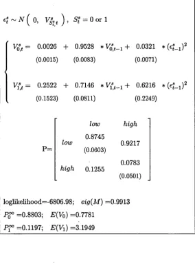
The estimation results of the univariate MS-GARCH model (2) using S&P500 daily returns are

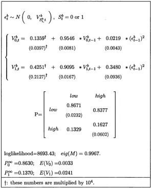
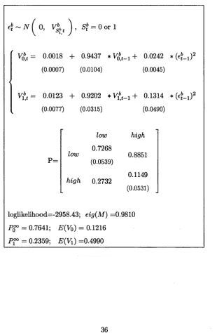
presented in Table 4, while Table 5 and 6 show the results for 1-year bond and 10-year bond

returns. The parameter estimates of the conditional mean are not shown, which will also applies to

other tables of the results. The same model has been estimated by Mittnik and Paolella (2004) on

foreign exchange returns. We find similar results on equity return data. First, there is a significant

difference in the persistence levels of the GARCH processes of the two regimes. When the volatility

process is in the low-volatility regime, the GARCH coefficient f3 is larger, but far away from unity,

which is usually the case when one fits a simple GARCH model to daily stock return data. The

ARCH coefficient a is much smaller than that of the high-volatility regime, less than one-tenth of

the latter6. So in tranquil periods, the volatility remains very stable, and the shock has very small

effect on the conditional variance of the next day. But in volatile periods, the impact of today’s

shock has much larger effect on next day’s conditional variance. The total persistence level of each

process are measured by the sum of a and /3. We could see in the table that in the low-volatility

regime, the GARCH process has persistence level smaller than unit, which means it is stationary.

But as found in Mittnik and Paolella (2004), the volatile regime has larger-than-unity persistence

level, so the GARCH process of the high-volatility regime itself is not stationary. The stationarity

of the whole system is determined jointly by the transition matrix and the two sets of persistence

parameters in both regimes, which is summarized by the largest eigenvalue of the matrix M, which

is explained in Appendix. We can see that all three univariate models are stationary with eig(M)

less than one. The stationary probability of low-volatility regime is higher than those found in

exchange return, which is mostly less than 0.8. The expected level of volatility in high-volatility

regime is about 4 times the expected level of low-volatility regime.

Table 5 and 6 report the estimation results of univariate MS-GARCH on the two bond return

series. The difference between the two regimes is similar to that found in stock index return. Higher

level of persistence, smaller (3 estimate and larger a estimate are associated with high-volatility

regime The persistence levels in the high-volatility regime of both bond series are larger than unity

as well. For 10-year bond returns the difference in /3 estimates is not significant. The difference

in (3 estimates for one-year bond is small as well, compared to that found in stock market. So for

bond market, the volatility dynamics of the two regimes mainly distinguish from each other in their

response to shocks. For one-year bond returns, the ratio of expected volatility in the high regime

to the low regime is much higher than that of the stock index return or ten-year bond return. Thus

the one-year bond would experience much larger jump upon regime-switching than stock return,

while 10-year bond behaves more similar to stock return.

5 .2 R e s u lts o n e s tim a tio n s o f th e jo in t m o d e l

We have studied the difference of the bond and stock markets in the univariate MS-GARCH model

in last section. Now we discuss their relation in the joint model. The joint model allows us to

see how the two state variables correspond to each other, and how the bond-stock correlation

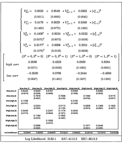
behaves within the 4 "combined states". First, we present the main estimation results of model (3)

using two pairs of stock-bond returns in Table 7 and Table 8. The first two blocks in the tables

are the regime-switching GARCH parameter estimates for the stock and bond series in the joint

estimation. The third block reports the constant correlation levels in each of the eight regimes.

The last block is the transition matrix estimate, together with the stationary probabilities of each

regime. In both tables, the estimates of GARCH parameters are similar to those from the univariate

estimations, but with smaller standard deviations due to efficiency increase by using more data.

And here we focus on the results on the joint part of the model. Then in Table 9 to Table 12,

relationships among the three latent processes. Finally, we have some discussions on the results of

the bond-stock correlations in a simple discounted cash-flow model for the bond and stock prices.

5.2.1 Stationary probabilities and correlations w ithin the combined states

First, we can indirectly see how likely the two volatility processes switch together by comparing the

stationary probabilities of the four "combined states". These can be obtained simply by summing

up the stationary probabilities of St states two by two. For the one-year bond pair, in about 76% of

time both the stock and bond return are in low-volatility regime, and in about 3.6% of time both of

them are in high-volatility regime. So there is about 20% of time that they are in different volatility

regimes. For the 10-year bond pair, the proportions of time that bond and stock volatilities are in

the same regime is similar to the one-year bond case. The main difference is that there is a much

larger percentage, about 8%, of time when both bond and stock are in high-volatility regimes. This

feature of ten-year bonds is a disadvantage for diversification. Large stationary probability of two

volatilities in the same regime for both pairs indicates that two volatility state variables correspond

to each other to a certain extent, which will be re-confirmed by the following results. We can also

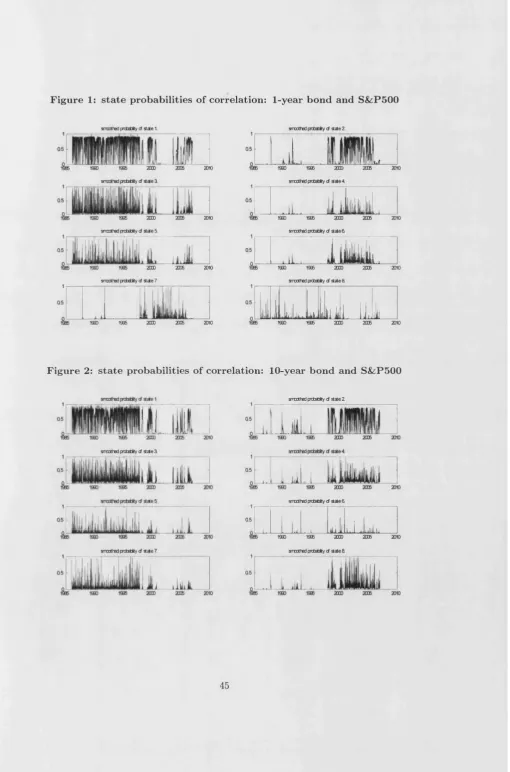
see the smoothed probabilities of each state across time in Figure 1 and 27.

Next, we compare the levels of correlation within the four "combined states". The two cor­

relation levels in the two "sub-states" of all four "combined states" are all significantly different.

These results indirectly suggest a separate state variable is needed for both stock-bond correla­

tion processes. Taking into account of estimation errors, only in the "low-stock-high-bond" state

are both of the two correlation estimates non-negative. And in the "high-stock-high-bond" state,

the high and low correlation estimates are the highest and lowest respectively among the eight

correlation estimates for the one-year bond paired with stock. Similar results are found for the

10-year paired with the stock. We will further discuss these findings in more details later. Finally,

for the one-year bond pair, taking into account of standard errors, we could see there are mainly

four correlation regimes: one extremely high at about 0.8, one negative at -0.4, and the other two

in between are around 0.35 and 0.05. A similar state reduction for correlation could be done for

ten-year bond pair, and we examine this formally in section 5.5.

5.2.2 C o n d itio n a l tra n s itio n p ro b ab ilities

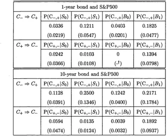
R e s u lts on th e t—co n d itio n al tra n s itio n p ro b a b ilitie s We study the intertemporal relations

between correlation state variable and the volatility state variables in two market through the

t — conditional transition probabilities reported in Table 9. Comparing these numbers with the

"unconditional transition probabilities" in Table 10 can reveal the forecasting benefit of allowing

correlation to have separate state variable. First, we look at the transition probabilities of Ct < 0 to

Ct+i ^ 0 given different volatility states in different markets. The correlation transition probability

is higher when conditional on high volatility state in either bond or stock than conditional on low

volatility state. And the difference is more significant for the one-year bond case. Comparing the

information contained in different markets, the correlation transition probabilities conditional on

low volatility states in two markets are not significant different for both pairs. However, correlation

transition probability conditional on high volatility states in one-year bond is larger than that

conditional on high volatility state in stock market. And for 10-year bond paired with stock

market, conditioning on either market produces similar correlation transition probabilities. So it

seems th at only correlation between the 1-year bond and stock has very different conditional "low to

high" transition probabilities for conditioning on different markets or different volatility states, and

the high volatility state of 1-year bond is mostly likely to be followed by a jump up in correlation.

Next, we turn to the transition probabilities of C* ^ 0 to Ct+i < 0 given various volatility

states. The correlation transition probability conditional on bond’s high volatility state is significant

higher than that conditional on bond’s low volatility state for both pairs. But the two volatility

states in stock market has similar information on the correlation transition probability, which is

different from above "high-to-low" case. Similar to the "high-to-low" case, there is no significant

difference in conditioning on the low volatility state of either stock or bond market for both pairs,

and conditioning on high volatility states in both bond markets has higher correlation transition

probabilities than conditioning on high volatility state in stock market.

To summarize, high volatility states of bond markets, especially 1-year bond, imply higher

t-conditional transition probabilities of bond-stock correlation for both "low-to-high" and "high-

to-low" cases. And the differences between these numbers and those "unconditional transition

probabilities" in Table 10 are statistically significant. But there is no significant difference in

regime-switching of the bond-stock correlation.

R e su lts on th e t + 1—co n d itio n al tra n s itio n p ro b ab ilities The contemporary relations

among the three state variables can be measured through the estimates of t + 1 — conditional

transition probabilities reported in Table 11. The first row of both panel is on how correlation

switches conditional on a regime-switching in bond or stock volatility, which can again be com­

pared with the unconditional ones in Table 10. For both bond pairs, when stock market volatility

jumps from low to high, the transition probabilities of correlation switching from high to low is

significantly higher than the unconditional ones while "high-to-low" correlation (conditional) tran­

sition probabilities are lower than the unconditional ones. However, conditioning on a "low-to-high"

jump in bond volatility has the opposite results: the correlation (conditional) transition probability

is higher, than the unconditional one for the "low-to-high" switching in correlation, and lower for

"high-to-low" case. So the "low-to-high" switching in stock volatility is more likely to be associated

with "high-to-low" switching in correlation while the "low-to-high" switching in bond volatility is

likely to be associated with "low-to-high" switching in correlation. The second row of both panels

evaluate how both of the volatility state variables switches conditioning on a regime-switching in

bond-stock correlation, which can be compared with the "unconditional (or marginal) transition

probabilities" in Table 4-6. The results are similar to those of first row since they inherit the main

properties of the quantities in first row by definition.

The last row of both panels describes how likely the two volatility processes would jump in the

same direction together. For ten-year bond, it tends to jump with stock in either direction with

high probability. But for one-year bond, it has high probability to jump down with stock, but very

low probability to jump up together. So the one-year bond does not always react the information

from stock market. But if it does react, probably to extreme shock, it resolves the uncertainty

together with stock market. Comparing these numbers to those in Table 4-6 also indicates that

only the case of "low-to-high" conditioning in the 1-year bond pair does not provide significant

more information than the marginal ones. So the two volatility state variables correspond to each

other quite well, especially for the 10-year bond pair.

The contemporary relationship revealed in above results indicate that the correlation state

variable has very different switching behavior from the volatility state variables while two volatility

S&P500.

5.2.3 C onditional expected correlations

An important feature of the general model is that it is able to capture the contemporary relations

among the correlation and volatilities in two markets. We quantify these relations through the

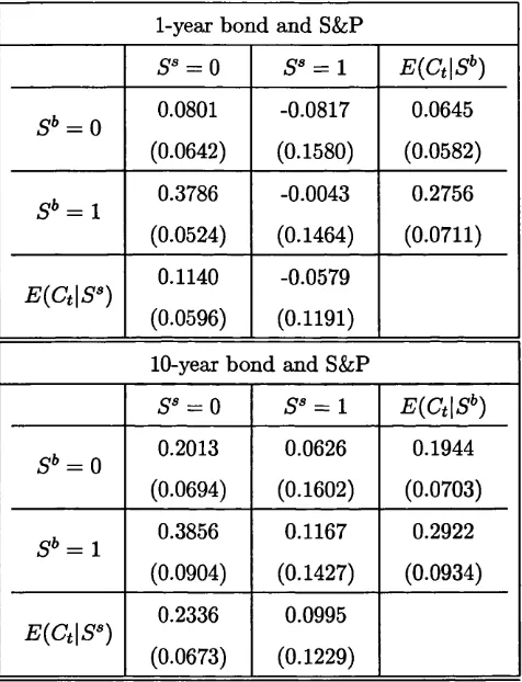
conditional expected correlations which are reported in Table 12.

First, we compare the expected correlations conditional on a single volatility state variable,

which are presented in the last row and column of both panels. For both pairs, the expected

correlation conditional on stock’s high volatility state is significant lower than that conditional

on stock’s low volatility state, although the difference is significant only for the 1-year bond pair.

But the results are opposite for those conditional on bond volatility states. Judging from the

differences in conditioning on high and low volatility-states, it seems that stock market has larger

contemporary impact on the bond-stock correlation than bond market. A related observation is

that only the expected correlation between 1-year bond and stock conditional on the high volatility

state in stock market has a negative point estimate. This reflects that during "flight to safety"

period, investors transfer money from stock market more to bonds with shorter maturities than

to bonds with longer maturities. This is again due to the fact that long-term bond is more like a

stock.

Table 12 also presents results on the "joint-conditional" expected correlations. These results

reveal the expected correlations in four "combined states", which is basically to aggregate the eight

correlation estimates from Table 7 and Table 8 into four correlation levels. For both pairs, the

"high-stock-low-bond" state has the lowest expected correlation while the "high-bond-low-stock"

state has the highest one. And in the most volatile market condition characterized as the "high-

stock-high-bond" state, the expected correlation is surprisingly low, even lower than the peaceful

"low-stock-low-bond" state. In the high stock volatility state, the difference in expected correlations

is not significant between conditioning on the high and low volatility states of the bond market.

But the difference is significant when the stock market is in low volatility state. In contrast, the

difference in the expected correlation is more significant between conditioning on stock’s high and

low volatility states when the bond market is in the high volatility state, especially for the 1-

year bond case. So when the stock market is very volatile, the bond-stock correlation is mainly

volatility on the bond-stock correlation becomes more prominent when the bond market is also in

volatile condition.

5.2.4 D iscussions on th e bond-stock correlations

Above empirical findings can be explained in a simple discounted cash-flow model for both the

bond and stock prices. The bond price is the expected value of the discounted factor while the

stock price is co-driven by the future cash flow and discount factor8. So the high bond-volatility

state is when the expected discount rate has high volatility. But for the stock volatility, it comes

from either one or both of the two shocks, cash-flow news and discount factor news. The recent

findings of Boyd, Hu and Jagannathan (2005) show that the stock price is dominated by the cash

flow effect during recessions while it mainly responds to discount rate news during expansions. Our

results are consistent with their findings. In the "high-bond-low-stock" state, the shock must come

form discount factor which will make the bond and stock prices move in same direction irrespective

of business cycle. This is confirmed by the result in Table 7. Only in the "high-bond-low-stock"

state can we have positive point estimates for both the high and low correlation states9. So when

we average them across the whole sample, we have highest unconditional correlation in the "high-

bond-low-stock" state as in Table 12.

However, for the "high-stock-high-bond" state, we have two different situations since the source

of the stock volatility is dependent on the business cycle. During expansions, both the bond and

stock prices are mainly driven by discount rate news. So we will have highest correlation during

expansions; But during recessions, the stock price is mainly dominated by the cash flow effect,

which works in the opposite direction for bond price as rising future cash flow will increase the

discount rate and lower the bond price. As a result, we have lowest bond-stock correlation during

recessions. This is confirmed by the regime correlation estimates in Table 7. And when we average

the correlations across the whole sample, the correlation is close to zero in the "high-bond-high-

stock" state as in Table 12. Results in the other two "combined states" can be explained similarly

by the relative effect of shocks to discount factor and cash flow in the discounted cash-flow model.

8 Different from discount factor for bond, the discount factor for stock is sum of equity premium and the risk-free rate. But for ease of illustration, we assume they are the same.

If we further differentiate the discount factors for the bond and stock prices, then the time-varying

equity premium will also help to explain the time-varying bond-stock correlations. This is especially

relevant for explaining the bond-stock correlation in sample after 2003 when it frequently swings

between large positive values and large negative values, which can not be explained by the business

cycle. A structural model is needed to measure the effect of time-varying equity premium on the

bond-stock correlation, which is out of the scope of this paper.

5 .3 E s tim a te d co r r ela tio n s from t h e M S C C C m o d el

Although we assume constant correlation within each regime, the correlation estimated from our

model has quite rich dynamics. Figure 3 and 4 provides the view of the correlation dynamic for

both pair over the past 20 years. Both correlations appear to jump to a negative level when there

is a crisis in equity market. As mentioned previously, since after 2003 negative correlations happen

very frequently, irrespective of having a stock market crisis or not. We believe it might be because

th at the time-varying equity premium is becoming more important for the bond-stock correlation

after 2003. As a comparison, we plot the MSCCC correlations together with correlations estimated

from DCC. As shown in Figure 5.1 and 6.1, the main difference between DCC’s correlations and

the MSCCC correlations is that the MSCCC correlations reveal more extreme, both positive and

negative, correlation level than the DCC. And forecast error in such situation are most costly

as pointed out by Engle and Collacito (2006). As another view for comparison, we fit the DCC

correlations by an 4-order polynomials of MSCCC correlations in Figure 5.2 and 6.2. We could see

DCC correlation usually has downward bias for day with high smoothed correlation, and upward

bias for day with low smoothed correlation. Although our model is not developed for forecasting, it

does point out potential way of improvement for the traditional GARCH type dynamic correlation

models, especially for modeling bond-stock correlation.

5 .4 R e s u lts o n r e s tr ic te d m o d els

Although all above analysis is based on the general model, we also estimate some restricted models

specified in Table 4 to compare their goodness of fit10. Table 13 reports the goodness-of-fit results

on all considered models. We rank all the model according to AIC and BIC. For one-year bond

pair, the most general model MSCCC(2,2,8), is the best model according to AIC. But according

to BIC, which penalize heavily extra parameters, MSCCC(2,2,4) is the best model, in which two

volatility process share the same Markov state variable but the correlation has a separate one. The

same best models are identified under the two criterion for ten-year bond paired with S&P500. So

generally according AIC, we do need three separate state variables for volatilities and correlation,

which justifies our main model. According to BIC the most general model still rank second for

the ten-year bond case, but very poorly for the one-year bond case. The MSCCC(2,2,4) is always

the best under BIC and the second under AIC. So while a separate state variable for correlation

is very important, stock and bond volatilities could share the same state variable without too

much loss in goodness of fit. This seems to reflect the information could be transmitted across

two markets efficiently within a day. The good performance of MSCCC(2,2,4) could also make it

a good candidate as a multivariate regime-switching GARCH model in forecasting exercise since it

is quite parsimonious, having only 28 parameters.

5 .5 D ia g n o stic a n a ly sis o f th e sta n d a rd ized residuals

In this section, we carry out the ARCH Lagrange multiplier (LM) test proposed by Engle (1982)

on the three residuals standardized by the conditional volatilities of the MSCCC model. As a naive

comparison, the same test is implemented for residuals standardized by conditional volatilities of

the DCC model. For all the tests, the number of lags is 5. The results are in Table 14. We can

see that the our regime-switching model has the p-values smaller than those of the DCC model

for almost all the lags for all three series. And only in the case of S&P 500 returns at the first

lag, the test statistics is significant only at 10% level for the MSCCC model. In contrast, the

DCC-standardized residuals have a significant statistics at 5% for the S&P return at the first lag.

From these results, we conclude that the proposed model has good performance in filtering out the

correlation in the return volatility,

6

C onclu din g R em arks

To study the bond-stock correlation and its relation with volatilities in the two markets, we extend

the univariate Markov-Switching GARCH of Haas Mittnik and Paolella (2004) into a bivariate

MS-GARCH model with Conditional Constant Correlation (CCC) specification. Our specification

allows a separate state variable governing each of the three processes: bond volatility, stock volatility

and bond-stock correlation, which is different from other multivariate generalizations of their model.

We estimate our model using two pairs of daily returns: S&P500 with one-year bond and S&P500

with ten-year bond, to study the difference in bond-stock correlation for different bond maturities.

From the univariate model estimation, we find both volatility processes switch between a sta­

tionary and a non-stationary state while the whole system is till stationary, similar to the findings

in Haas Mittnik and Paolella (2004). By allowing different latent process to have separate Markov

state variable, the results from the joint model estimation has the following main findings: First, we

find that a separate state variable for the bond-stock correlation is needed while the two volatility

processes could largely share a common state variable, especially for the 1 0-year bond paired with

S&P500. Second, the "low-to-high" switching in stock volatility is more likely to be associated with

the "high-to-low" switching in correlation while the "low-to-high" switching in bond volatility is

likely to be associated with the "low-to-high" switching in correlation. As a result, we show that the

expected bond-stock correlation conditional on stock’s high volatility state is significant lower than

that conditional on stock’s low volatility state. But the results are opposite for those conditional

on bond’s volatility state. Finally, we find that when the bond market is in its high volatility state

and the stock market is in its low volatility state, the estimates of bond-stock correlation in both

high and low correlations states are non-negative. But when both bond and stock markets are

in high volatility state, the bond-stock correlation has the highest correlation estimate at its high

correlation-state and almost lowest correlation estimate at its low correlation-state. This might be

attributed to the relative impacts of shocks to the cash flow and shocks to the discount factor on

the pricing of bonds and stocks at different stages of business cycles. But we also find large swings

in the bond-stock correlation between positive and negative values after 2003, which can not be

explained by the business cycle, and possibly can be driven by the time-varying equity premium.

The proposed model assumes constant correlation within each state. The estimate correlations

within each state. So modeling the correlation as two-state regime-switching DCC may be adequate

to capture both the structural break in the level of the correlation and the variation within each

regime. Future work will consider how to effectively incorporate DCC in this regime-switching

GARCH framework in a way that is parsimonious and numerically tractable. A better covariance

forecasting model could also be developed in a similar approach. Another interesting research topic

will be comparing the filtered states with the macro news announcement. For example, the state-7

should be related to the discount rate news in expansion while state- 8 should be related to cash

flow news in recession. Finally, our model might also be applied to study the contagion effect in

A p p en d ix: D eta ils

A l : d e ta ils o f m a x im u m lik e lih o o d e s tim a tio n

The general model could be estimated by maximum likelihood method. The algebra is standard, as

in Hamilton (1994). Let 0 = a*, /3 PijCi} w ith i = 1,2. . . 8 and k = s or b, be the parameter

space of model (3). And is the whole history of return from 0 to t. Then the likelihood of the

observed return pairs at time t can be written as:

N

= s t = i | e ; 4 _ w ])

i=1

N

= £ > w , i # 0 ; St = i; 4 _ li0]) * Pr(St = i|0 ; JJft_ li0], J $ _ li0])

1=1

N N

= flf|0 ; S, = <; flft_li0J) * 5 > r ( S t = <|6 ; S t- i = j ) * Pr(S«-i = j |0 ; 4 _ i , 0])]

t=l j=1

N N

= * f