Economic development and the
environment: three essays
Stefanie Sieber
Dissertation submitted for the degree of Doctor of Philosophy in Economics at
The London School of Economics and Political Science
UMI Number: U615B42
All rights reserved
INFORMATION TO ALL U SE R S
The quality of this reproduction is d ep en d en t upon the quality of the copy subm itted.
In the unlikely even t that the author did not sen d a com plete m anuscript
and there are m issing p a g e s, th e se will be noted. Also, if material had to be rem oved,
a note will indicate the deletion.
Dissertation Publishing
UMI U615B42
Published by ProQ uest LLC 2014. Copyright in the Dissertation held by the Author.
Microform Edition © ProQ uest LLC.
All rights reserved. This work is protected against unauthorized copying under Title 17, United S ta tes C ode.
ProQ uest LLC
789 East E isenhow er Parkway
Library
British Library o f Political a n d E c o n o m ic S c ie n c eD eclaration
2
I certify th a t the thesis I have presented for examination for the PhD degree of the
London School of Economics and Political Science is solely my own work other than
where I have clearly indicated th a t it is the work of others. The second chapter
draws on work th a t was carried out jointly with equal share by Robin Burgess (LSE),
Matthew Hansen (South Dakota State University), Benjamin Olken (Massachusetts
Institute of Technology), and me.
The copyright of this thesis rests with the author. Quotation from it is perm itted,
provided th at full acknowledgement is made. This thesis may not be reproduced
without the prior w ritten consent of the author.
I warrant th a t this authorisation does not, to the best of my belief, infringe the
rights of any third party.
A bstract
3
The main question th a t motivates my PhD thesis is how economic activity in devel
oping countries is influenced by and, in turn, affects the environment. Since these
interactions can take many forms, I investigate this issue from three different angles,
which necessitates both the usage of novel remote-sensing-based datasets and the de
velopment of a new theoretical framework.
Firstly, the environment can have a direct impact on economic development, the
most obvious example being natural disasters like cyclones. As the incidence and
intensity of these events will increase with climate change, it is crucial to estimate
their short- and long-run costs and the behavioural response of producers to these
large and mostly uninsured aggregate shocks. I have, thus, created a new digital
database of cyclone exposure for India to estimate how farmers smooth income in the
afterm ath of these events.
The causality can also run the other way, as economic agents disrupt the environ ment. A case in point is deforestation, which is analysed in the co-authored second
chapter of my thesis. In particular, we use satellite d ata to study how political decen
tralisation has affected district-level logging rates in Indonesia. Possible mechanisms
include local election cycles, the move from monopoly to oligopoly or the need to raise
revenue in the absence of other natural resources.
Finally, the third chapter assesses to what extent the environment can create pre
conditions for socioeconomic interaction. More specifically, I analyse how the intro
duction of heterogeneous space into the standard urban Muth-Mills model generates a
residential equilibrium where the formal and informal housing markets coexist. This
new setup is then used to evaluate the usual policy prescriptions for slums and demon strates th a t new insights can be gained by adding the spatial component.
This thesis, therefore, explores possible links between the environment and eco
nomic development and illustrates the advantages of using methods and d ata sources
For my grandfather, Peter Bahles senior, without whom I could have never studied
5
A cknowledgem ents
There are many whose help was invaluable for me in completing my PhD thesis.
I would like to thank my primary supervisor Robin Burgess for his inspiring ideas
and generous advice. My secondary supervisor Oriana Bandiera deserves my thanks
for prolific discussions and the great amount of time she has devoted to my thesis,
especially in its final stages. Benjamin Olken from MIT was very helpful in getting
me started on my first chapter and has been a great source of learning throughout the
work for our joint project, which constitutes the second chapter of this thesis.
I am also deeply indebted to the LSE for awarding me the full Tibor Scitovsky
Scholarship and a one-year Economic Research Studentship th a t allowed me to con
duct my research. Financial support from the DFID Research Program Consortium on
Improving Institutions for Pro-Poor Growth in Africa and South-Asia is also gratefully
acknowledged.
I would also like to thank Matthew Hansen from the Geographic Information Sci
ence Center of Excellence at SDSU for sharing his remote sensing d ata and expertise.
The second chapter of this thesis would not have been possible without his help. Mark
Broich has also provided kind and patient explanations. Furthermore, Raymond Gui- teras has been extremely helpful in sharing the World Bank India Agricultural and
Climate Dataset with me.
Moreover, I would like to thank my wonderful proof-readers, Christine Knoop and Jennie Condell, without whose input my work could not have become what it is. Any
linguistic infelicities th a t may have found their way into th e text despite their best
efforts are, of course, my responsibility.
There are a number of others who contributed to this thesis less directly, but
no less significantly. I would like to thank Dave Donaldson, Esther Duflo, Cynthia
Kinnan, Guy Michaels, Henry Overman, Rohini Pande, Olmo Silva, Daniel Sturm,
Anthony Venables, and seminar participants at the LSE for helpful comments and
discussions. This work has also benefitted from my stay at MIT and the Jameel
Abdul Latif Poverty Action Lab from September 2008 to August 2009.
Many thanks are also due to the incredibly helpful IT team at STICERD, Joe
Joannes and Nic Warner, whose continued support and assistance made the empirical
work for the second chapter possible. Mahvish Shaukat and Nivedhitha Subramanian
have provided excellent research assistance for the same project.
In addition, I would like thank my friends for their support, assistance, and pa
tience throughout my doctoral studies. Above all, I would like to thank my best friend
Christine Knoop for her encouragement and thought-provoking impulses in the many
phases of this thesis. I could not have completed it w ithout her.
Last but not least, I would like to thank my dear family, my parents K atja and
Michael Sieber, my brother Oliver and his wife Virginie, for their unwavering support
6
C ontents
A b stra ct 3
A cknow ledgem ents 5
C on ten ts 6
List o f Figures 9
List o f Tables 10
P reface 11
1 Incom e S m ooth in g and C y clon e D am age in In dia 14
1.1 In tro d u ctio n ... 14
1.2 B ack g ro u n d ... 16
1.3 D a t a ... 18
1.3.1 Cyclone d ata so u rc e s... 19
1.3.2 Measuring cyclone exposure at the district le v e l... 20
1.3.3 D ata for the prim ary s e c t o r ... 22
1.4 Identification s t r a t e g y ... 24
1.4.1 Motivation ... 24
1.4.2 Empirical Im plem en tation... 25
1.5 R esu lts... 27
1.5.1 The net effect of tropical cyclones on agricultural production . 27 1.5.2 Coping strategy 1: income smoothing across growing seasons . 29 1.5.3 Coping strategy 2: changes in the crop mix towards cheap calories 30 1.6 Conclusion ... 31
A D ata a p p e n d i x ... 33
A .l The district sam p le... 33
A.2 The tropical cyclone wind speed buffers dataset, 1975-2007 . . 33
A.3 The eAtlas cyclone tracks dataset, 1891-2008 ... 34
A.4 The data for the prim ary sector, 1956-1987 ... 35
A.5 The crop c a l e n d a r ... 36
2 T h e P o litica l E conom y o f Tropical D efo resta tio n 52 2.1 Intro d u ctio n ... 52
2.2 Background and D a t a ... 55
2.2.1 B ackg ro un d... 55
2.2.1.1 Decentralisation in Post-Soeharto Indonesia... 55
2.2.1.2 Implications for the Forest S e c t o r ... 56
C O N TE N TS 7
2.2.2.1 Constructing the satellite dataset ... 58
2.2.2.2 Descriptive statistics of forest c h a n g e ... 61
2.2.2.3 Political Economy D a t a ... 62
2.3 Cournot competition between d i s t r i c t s ... 63
2.3.1 Theory ... 63
2.3.2 Empirical T e s ts ... 64
2.3.3 Results using official production s t a t i s t i c s ... 67
2.3.3.1 R e s u l t s ... 67
2.3.3.2 Alternative sp ecificatio n s... 68
2.3.4 Results using the satellite d ata at the province l e v e l ... 69
2.3.5 Results for the satellite d ata at the district l e v e l ... 70
2.4 Political logging c y c le s ... 72
2.4.1 Empirical t e s t s ... 72
2.4.2 Results ... 73
2.5 Substitutes or complements? Logging vs. other sources of rents . . . . 74
2.5.1 Empirical im p lem en tatio n ... 74
2.5.2 Results ... 75
2.6 C on clusion s... 76
B D ata a p p e n d i x ... 78
B .l Government forestry d a t a ... 78
B.2 District split data ... 78
B.3 District election d a t a ... 79
B.4 District public finance d a t a ... 79
3 A n A m en ity-b ased T h eory o f S q u atter S e ttlem e n ts 98 3.1 In tro d u ctio n ... 98
3.2 Basic m o d e l... 101
3.2.1 The s e t u p ... 101
3.2.2 The formal housing m a r k e t ... 103
3.2.3 The informal (squatting) housing market ... 105
3.3 The extended m o d e l ... 109
3.3.1 The location by income in the formal housing market... 110
3.3.2 Possible residential equilibria in the formal housing market . . 112
3.3.3 The location by income in the informal housing market and the final residential e q u ilib riu m ... 114
3.4 Policy a n a l y s i s ... 118
3.4.1 The effect of a slum-upgrading program on the residential equi librium 118
C O N TE N TS 8
3.4.1.2 Scenario 2: public investment into the amenity level
of the s q u a t... 124
3.4.2 The effect of greater security of tenure on the residential equi
librium ... 126
3.5 Conclusion ... 128
C A p p e n d ix ... 130
C .l Derivation of the bid rent curve and its slope in the formal
housing market; example: Cobb-Douglas u t i l i t y ... 130
C.2 Derivation of the slope of the bid rent curve in the informal
housing m a r k e t... 131
C.3 The effect of a change in income on the slope of the bid rent
curve in the formal housing market; example: Cobb-Douglas
u t i l i t y ... 132 C.4 The effect of a slum-upgrading program on the bid rent curve
in the formal housing market; example: Cobb-Douglas utility . 133 C.5 The effect of a slum-upgrading program on the bid rent curve
in the informal housing m a r k e t ... 134
9
List o f Figures
1.1 UNEP wind speed buffers and eAtlas cyclone tracks, 1977-2003 . . . . 37
1.2 Correlation between the % area exposed as measured by the UNEP wind speed buffers and as predicted by the eAtlas cyclone tracks, 1977- 2003 ... 38
1.2 Correlation between the % area exposed as measured by the UNEP wind speed buffers and as predicted by the eAtlas cyclone tracks, 1977- 2003 ... 39
1.2 Correlation between the % area exposed as measured by the UNEP wind speed buffers and as predicted by the eAtlas cyclone tracks, 1977- 2003 ... 40
1.3 Distribution of the % area exposed as measured by the UNEP wind speed buffers and as predicted by the eAtlas cyclone tracks, 1977-2003 41 1.3 Distribution of the % area exposed as measured by the UNEP wind speed buffers and as predicted by the eAtlas cyclone tracks, 1977-2003 42 1.3 Distribution of the % area exposed as measured by the UNEP wind speed buffers and as predicted by the eAtlas cyclone tracks, 1977-2003 43 2.1 Forest cover change in the province of Riau, 2001-2008 ... 80
2.2 District-level logging in Indonesia using the 2008 district boundaries . 81 2.2 District-level logging in Indonesia using the 2008 district boundaries . 82 2.3 Total number of district splits using the 1990 district boundaries, 1990- 2008 ... 83
2.4 Oil and gas revenue per capita using the 2008 district boundaries, 2008 84 3.1 The amenity-level as a function of distance ... 102
3.2 The bid-rent curve in the formal housing m a r k e t ... 105
3.3 Possible intersections of the bid-rent curve for the high- and middle- income h ou sehold... I l l 3.4 Possible residential equilibria with no vacant p l o t ... 113
3.5 Possible residential equilibria: with a vacant p l o t ... 114
3.6 The final residential equilibrium with squat f o r m a t io n ... 117
3.7 An improvement in the amenity level for x < x < x ... 119
3.8 The effect of an investment in the amenity level of x < x < x on the bid rent curves in the formal housing market ... 121
3.9 The effect of a private investment in the amenity level of x < x < x on the residential eq u ilib riu m ... 123
10
List o f Tables
1.1 Summary statistics of the cyclone exposure variables, 1956-87 ... 44
1.2 The net effect of a cyclone s h o c k ... 45
1.3 A falsification e x e rc is e ... 46
1.4 The impact of cyclones on winter crops ... 47
1.5 The impact of cyclones on summer c ro p s ... 48
1.6 The impact of cyclones on coarse c e re a ls ... 49
1.7 The impact of cyclones on all other food crops ... 50
A .l The net effect of a cyclone shock: alternative cyclone variables . . . . 51
2.1 Forest area in 1000 H A ... 85
2.2 Summary statistics of forest area cleared in 1000HA by districtXyear . 86 2.3 Impact of Splits on Prices and Quantities: Legal Logging D ata . . . . 87
2.4 Impact of Splits on Prices and Quantities: Alternative Specifications . 88 2.4 Impact of Splits on Prices and Quantities: Alternative Specifications ( c o n t.) ... 89
2.5 Satellite data on impact of splits, province le v e l... 90
2.6 Satellite data on impact of splits with leads, province le v e l... 91
2.7 Satellite data on impact of splits, district level ... 92
2.7 Satellite data on impact of splits, district level (cont.) ... 93
2.8 Satellite data on impact of splits with leads, district l e v e l ... 94
2.8 Satellite data on impact of splits with leads, district level (cont.) . . . 95
2.9 E lections... 96
Preface
11
The issue of economic activity in developing countries being influenced by and, in turn,
affecting the environment has come to the forefront of public debate. The discourse has
been fuelled by recent research on anthropogenic climate change, which has shown th a t
livelihoods all over the world will be threatened if environmental concerns continue to
be ignored (IPCC, 2007a). It is therefore crucial to understand the linkages between
economic activity and the environment if we are to draw wider conclusions on ways
to decelerate climate change and mitigate its consequences. My PhD thesis explores
three of these many conceivable linkages.
Until recently, research in this field has been restricted due to limited availability
of relevant data. Now remote sensing technologies have opened up new d ata sources
to economists and can be used to measure natural phenomena objectively in real time.
This kind of data is particularly valuable for analyses of developing countries, for which
the record is often incomplete. Moreover, satellite images provide a comprehensive picture of the earth’s surface and therefore are able to capture the impact of both
legal and illegal actions on the environment.
The first two chapters of this thesis make use of these novel d ata sources to analyse
two possible linkages between the environment and economic activity. The environ ment can have a direct impact on economic development, the most straightforward
example being the destruction of agricultural output caused by natural disasters. De
veloping countries are particularly vulnerable to these shocks, because their economies
depend heavily on the primary sector (FAO, 2009). Given th a t the frequency and intensity of extreme weather events are predicted to increase with climate change
(Christensen et al., 2007), it becomes all the more im portant to estimate the associ
ated short- and long-run costs.
Chapter 1 studies the impact of one particular natural disaster, namely tropical
cyclones. I construct a new digital database of cyclone exposure for India, which I
use to estimate the effect of these shocks on the prim ary sector. In addition, the
disaggregate nature of the agricultural d ata allows me to take the analysis further
and study how producers recover from these large and mostly uninsured aggregate
income shocks. More specifically, I exploit the interaction between the random timing
of the cyclone hit and the district-level growing seasons to identify possible income
smoothing mechanisms. I find th a t producers smooth income both by increasing their
production in the growing season immediately following the cyclone shock and by
changing their crop mix towards more resilient and nutritious crops.
However, the causality can also run the other way, as economic agents disrupt and
destroy the environment. A case in point is deforestation, which is one of the main
drivers of anthropogenic climate change (Denman et al., 2007). It is thus im portant to understand how forests can be preserved effectively, as sustainable forest management
Nabu-PREFACE 12
urs et al., 2007). This policy issue is again especially relevant for developing countries,
whose weak institutions can lead to excessive illegal logging (CIFOR, 2004), which will
have to be curbed if emissions are to be reduced.
Indonesia provides an insightful case study, as it is experiencing some of the most
rapid deforestation rates in the world (Hansen et al., 2009). Furthermore, it has
concomitantly experienced fundamental institutional changes since the overthrow of
the dictator Soeharto. The co-authored second chapter of my thesis thus uses a new
satellite-based forest cover dataset to investigate how decentralisation has affected
deforestation. We analyse a series of possible political economy mechanisms and
find th a t the move from a monopoly of forest extraction rights to an oligopoly has
significantly increased logging. Moreover, fiscal decentralisation has incentivised local
bureaucrats and politicians to raise revenue through logging. This is particularly the
case prior to local elections or if districts do not have access to other lucrative natural
resources, such as oil and gas.
Finally, given th a t climate change will destroy rural livelihoods, especially in de veloping countries (IPCC, 2007a), th e pressure on urban areas is set to increase over
the coming decades. Since city governments in these regions have limited resources
to finance public housing schemes (Simha, 2006; WB, 2002), this will drive the new
arrivals into the informal housing market. A variety of policy prescriptions involving
slum-upgrading and titling programmes have been offered to tackle this looming hous ing crisis (UN-Habitat (2003), chapter 7). However, the consequences of these policies
can only be fully understood if the analysis is integrated into a spatial context; an
aspect which has been ignored so far.
The third and final chapter of my thesis addresses this issue by studying how the environment can create preconditions for socioeconomic interaction. More specifically,
Chapter 3 provides a new theoretical framework th a t introduces heterogeneous space
into the standard urban model of the monocentric city. This generates a residential
equilibrium where the formal and informal housing markets coexist; a feature th a t
is assumed to be exogenously given in other models (Jiminez, 1984; Brueckner and
Selod, 2008). This new setup is then used to evaluate the usual policy prescriptions
for slums and demonstrates th a t new insights can be gained by adding the spatial
component. In particular, the results suggest th a t slum upgrading is economically
inefficient and th a t resettlement programmes could increase social welfare.
The three chapters of this thesis thus contribute to the wider debate on how our
economic decisions both axe influenced by and impact upon the environment, and, by
extension, anthropogenic climate change. The first chapter provides some evidence
on possible coping strategies in the face of extreme weather events that disrupt the
usual insurance arrangements. Given th a t global warming will increase the likelihood
of such aggregate shocks, the focus of both academics and policy makers should shift
more towards understanding income smoothing mechanisms. In contrast, the second
PREFACE 13
The findings suggest th a t logging rates can only be lowered with a comprehensive
policy approach th a t also addresses institutional weakness. Lastly, the third chapter
deals with the consequences of actual displacement through climate change, which will
transm it the impact of global warming from the rural to the urban sphere. As these
population pressures will significantly increase in the coming decades, early action is
warranted to create the capacities to accommodate this influx.
Given the complexity of the problem, future research should devote more effort to
understanding the multifaceted relationship between the environment and economic
activity. Only then will we be able to devise possible adaptation and mitigation
strategies th at will help lower the costs of anthropogenic climate change both for
14
1
Incom e Sm oothing and Cyclone
D am age in India
1.1 I n tr o d u c tio n
Tropical cyclones axe some of the most devastating natural disasters on the earth
(Dilley et al., 2005). They are intense whirls in the atmosphere th a t reach wind
speeds of up to 250km/h - the average speed of a TGV (Taylor, 2007). These storms
usually affect large areas, as a fully-grown cyclone can have a diameter of 1,000km and
move 300 to 500km in a day (IMD, 2009). In addition, they are often accompanied
by storm surges and torrential rains, which inundate coastal regions and flood rivers.
The resulting destruction can be apocalyptic. For instance, the 1999 Orissa cyclone -
the deadliest Indian storm since 1971 - affected 17,993 villages in 14 districts (BAPS,
1999). Official figures p ut the death toll at 9,893 (though it is believed th a t as many as 15,000 people died) and estimated a cost of approximately US$4.5 billion. Moreover,
around 5 million farmers lost their livelihoods, since 406,000 farm animals perished in
the storm and 1.7 million hectares of crops were destroyed (USNO, 1999).
The destructive potential of tropical cyclones is bound to increase even further. In
fact, climate change models predict a higher frequency and intensity of these storms over the next few decades (Henderson-Sellers et al., 1998; Kuntson and Tuleya, 2004;
Emanuel, 2005; Christensen et al., 2007). Developing countries in particular will
suffer disproportionately from this development. Empirical evidence has shown th a t
the impact of natural disasters is larger for poorer, more unequal, and less democratic
societies (Khan, 2005; Stromberg, 2007; Toya and Skidmore, 2007). Furthermore, their economies heavily depend on the prim ary sector, which is affected most by cyclones.
Recent figures for India, for example, show th at 56.35% of the economically active
population work in agriculture whose share in GDP is 16.6% (comparable figures for
the US are 1.75% and 1.1% respectively) (FAO, 2009).
Given the importance of the issue, this paper’s main aim is to estimate the cost of
tropical cyclones on the primary sector in developing countries. In addition, I inves
tigate possible mechanisms through which farmers try to cope with these aggregate
income shocks. I focus on one country - India - th at is struck by a tropical cyclone
every two to eight years on average. The great advantage of this case study is th a t the
India Meteorological Department has recorded the positions of all cyclones since 1891.
I can thus construct a novel dataset of cyclone exposure, which estimates the disaster
impact for a long time horizon in a consistent and objective manner (O’Keefe and
Westgate, 1976; Albala-Bertrand, 1993; Yang, 2008). This dataset is then combined
with the India Agriculture and Climate D ataset of the World Bank - the most com
prehensive district panel of agricultural data currently available for India. Specifically,
1 INCO M E SM OOTHING A N D C YC LO N E D AM AG E IN INDIA 15
Using these two datasets, I can estimate the cost of tropical cyclones on a much
finer geographical scale than has been feasible previously.1 I find th a t a one standard
deviation increase in cyclone exposure lowers output by 7.75%. Rather surprisingly, I
also find th a t the area planted increases contemporaneously by 3.02%; an effect which persists for three years until recovery is achieved. These seemingly contradictory
results can be explained by the following observation: most districts in India have
two and some even three growing seasons (GOI, 1967). T h at is to say, producers will
be able to adjust their production later in the same year, if, for instance, they were
struck by a cyclone in the spring. The annual d ata thus only captures the net effect of
the natural disaster, where the destruction caused by the cyclone is counterbalanced
by the subsequent behavioural response of the producers.
The change in behaviour in itself is warranted, because most farmers are not pro
tected against cyclone shocks. Firstly, the Indian government only provides short-term
disaster relief th a t does not involve any aid for recovery or development (Parasuraman
and Unnikrishnan, eds, 2000). Secondly, most producers lack formal insurance against
weather risk, which is rarely taken out in both developed and developing countries
(Kunreuther and Pauly, 2004; Cole et al., 2009). Finally, since the cyclone affects
the entire social network, access to informal finance will be disrupted (Besley, 1995a). Consequently, farmers will be unable to smooth consumption in the afterm ath of the
natural disaster and will have to adjust their production behaviour instead.
Due to the detailed nature of my dataset, I can identify two possible coping strate
gies th a t could explain the observed increase in the area planted. Firstly, the anal ysis exploits the interaction between the random timing of the cyclone shock and
the district-level growing seasons. More specifically, I supplement the World Bank’s
dataset with district-level growing cycle information to distinguish between cyclone
events th a t happen before and after the sowing season of each individual crop. I can
then test whether production increases after the previous harvest has been destroyed.
The results show a very consistent picture - a crop is destroyed if the cyclone hits prior
to the harvest, but more is planted if it strikes before the sowing season. Farmers thus
attem pt to smooth income by substituting intertemporally across growing seasons.
Note th a t the effectiveness of this coping strategy will be dampened, since markets
are not well-integrated in India (Topalova, 2004; Duflo and Pande, 2007; Guiteras,
2007). This is confirmed in the data, as local farm harvest prices decline with the
expansion in production.
The second income smoothing mechanism involves a change in the crop mix. In
particular, I separate the food crops into two main groups. The first category com
prises coarse cereals, such as b ajra and jowar. These crops are resilient, cheap, and
highly nutritious. The second group includes more risky and expensive calories like
rice and wheat. If farmers need to smooth income and (most probably) nutrition
1 INCO M E SM OOTHING AN D C YCLO NE DAM AGE IN IND IA 16
after the cyclone shock, we would expect to see a switch towards coarse cereals. The
evidence suggests th a t this is indeed the case - the area planted with coarse cereals ex
pands by 4.22% resulting in a net increase in output and a decline in prices of 11.47%
and 2.53% respectively. In contrast, the other food crops are largely destroyed by the
cyclone (output drops by 13.93%) and are not replanted within the same year. This
finding can also explain the overall increase in the area planted, since coarse cereals
can be grown on marginal land whereas other food crops cannot (Sawhney and Daji,
1961). Farmers thus seem to forgo higher income from low calorie crops to meet basic
nutritional needs and smooth income after the cyclone shock.
These results document the large and adverse impact of tropical cyclones on the
primary sector in India. I find th a t producers attem pt to counter the destruction
- by planting more crops in the growing season directly following the cyclone shock
or by changing their crop mix towards cheap calories. However, their response is
not sufficient. The overall contemporaneous impact on output is still negative and
sizeable. Moreover, income smoothing continues for another three years until the
damage is offset completely. Disaster relief should thus not only provide short-term
supportive measures, but also assistance to rebuild livelihoods. Furthermore, it is
im portant to note th a t these coping strategies are specific to India. The impact of
cyclonic storms will be larger for developing countries with only one growing season. The remainder of the paper is organized as follows. In the next section, I discuss
the related literature and place the contribution of this paper in a broader context.
Section 1.3 explains how the cyclone exposure dataset is constructed and discusses the key features of the World Bank dataset needed for the empirical analysis. In Section
1.4, I motivate the identification strategy and describe its empirical implementation.
Section 1.5.1 presents the estimates of the net effect of cyclone exposure on the primary
sector. In Section 1.5.2, I study how the interaction between the district-level growing
seasons and the timing of the cyclone shock affects planting decisions. Section 1.5.3
tests if the crop mix changes in response to tropical cyclones. Section 1.6 concludes.
1.2 B a c k g r o u n d
This paper is most closely related to the nascent literature on natural disasters. Re
search in this field has so fax largely focused on estimating the impact of these aggre
gate shocks at the macro-level (Toya and Skidmore, 2002; Stromberg, 2007; Cuaresma
et al., 2008). A prominent cross-country analysis has been carried out by Khan (2005),
who shows th at good institutions and democracies can play a crucial role in lowering
the death toll from natural disasters. Similarly, Anbarci et al. (2005) provide evidence
th a t richer and more equal societies have fewer fatalities.
However, even if this relationship is true across countries, recent micro-evidence
paints a more nuanced picture. For instance, Pugatch and Yang (2008) show nonlin
1 INCO M E SM OOTHING AN D CYCLO NE D AM AG E IN INDIA 17
opment. They argue th a t reconstruction efforts in more affluent regions have induced
emigration from poorer to richer states, thus mitigating the impact for both. In ad
dition, more aid is usually provided by more accountable local governments (Besley
and Burgess, 2002; Cole et al., 2008) or for natural disasters with wider media cov
erage (Eisensee and Stromberg, 2007). The impact also differs across income groups,
since families with lower levels of education (Bluedorn and Cascio, 2005) and income
(Foster, 1995) suffer most.
The present study contributes to this literature by estimating the effect of tropical
cyclones on the primary sector in India. By exploiting the finesse of my cyclone
dataset, I am able to estimate this effect for each district - a level of disaggregation
which has not been achieved before. The reasons for focusing on the primary sector are
as follows. Firstly, agricultural production is most exposed to cyclonic storms. The
strong winds, and accompanying rains and floods will primarily destroy crops and kill
livestock (IMD, 2009). Secondly, more than half of the economically active population
in India (and in most other developing countries) works in agriculture today (FAO,
2009). Therefore, the full impact of this natural disaster can only be understood if the prim ary sector is taken into account.
Moreover, to the best of my knowledge this paper attem pts to disentangle possible
coping strategies for the first time. So far, little empirical evidence exists on how
producers recover from aggregate income shocks like natural disasters. For instance, the related literature on large temporary shocks merely studies their long-run impact.
A case in point is the analysis of Miguel and Roland (2006). They show th a t the ex
tensive bombing of Vietnam has not permanently changed poverty rates, consumption
patterns, infrastructure, literacy, and population density. However, they cannot iden
tify the mechanisms through which recovery has been accomplished. Similarly, Davis
and Weinstein (2002) provide evidence th a t the dropping of the atomic bombs on Hi roshima and Nagasaki has not had a long-run impact on the distribution of economic
activity in Japan. But again evidence on possible coping strategies is scarce.2
Given th a t natural disasters repeatedly strike the same region (Dilley et al., 2005),
we would expect th at forward-looking economic agents will insure themselves against
these shocks. Nonetheless, empirical evidence has shown th a t households underin-
sure against weather risk due to incomplete information about the event probability
(Kunreuther and Pauly, 2004), credit constraints, and lack of trust (Cole et al., 2009).
In the case of India, government assistance is not sufficient to offset the negative
consequences of natural disasters either. That is, relief operations largely focus on
short-term supportive measures and not on recovery and development (Parasuraman
and Unnikrishnan, eds, 2000; HPC, 2001).3
2In contrast to these temporary one-off shocks, permanent changes in the productive capacity of a region should lead to a behavioural response. For example, Hornbeck (2008) finds that migration patterns and population growth changed substantially in response to the extensive topsoil erosion in the American Dustbowl.
1 INCO M E SM OOTHING AN D CYC LO NE DAM AGE IN INDIA 18
Alternatively, producers could insure themselves more indirectly through bor
rowing and saving. The academic literature has provided considerable evidence on
consumption smoothing through both formal and informal credit arrangements in
developing countries (Deaton, 1992; Udry, 1994; Townsend, 1994; Grimard, 1997;
Fafchamps and Lund, 1997; Dubois, 2000). Yet, the findings suggest th a t this is
far from complete. Moreover, informal insurance networks are particularly vulnerable
to geographically co-moving shocks like tropical cyclones. In particular, they usually
rely on local information networks and community sanctions to overcome information
asymmetries, enforcement problems and transaction costs (Besley, 1995a). Since the
cyclone will affect the entire social network, producers will be severely limited in their
ability to smooth consumption through borrowing.
In such an environment of repeated and largely uninsured aggregate shocks, pro
ducers will have to fall back on income smoothing mechanisms (Morduch, 1995).
This literature is much more limited, as most of the research to date has focused on
household-level borrowing and saving behaviour. The existing evidence suggests th a t farmers attem pt to smooth income by selling their assets or livestock or by increasing
their labour supply or off-farm employment (Rosenzweig and Wolpin, 1993; Dercon,
2000; Jayachandran, 2006). However, this will be more difficult after a cyclone shock,
which will have damaged assets, killed domestic animals, and severely disrupted the
local economy. Moreover, the effectiveness of these coping strategies will be reduced if markets are not well integrated. This is the case in India (Topalova, 2004; Duflo
and Pande, 2007; Guiteras, 2007), where we would expect general equilibrium effects
to drive down local prices and wages.
This paper studies two alternative income smoothing mechanisms: namely, changes
in the crop mix and an increase in agricultural production in the subsequent growing season. Naturally, these responses will also have local price effects, which will mitigate
their impact. However, they might be easier to implement after a natural disaster. To
identify these coping strategies, I take advantage of the detailed nature of my dataset.
More specifically, I can determine whether a cyclone shock has occurred before or
after the district-level sowing season of a given crop. The behavioural response will
be identified by cyclone hits prior to the sowing season. In contrast, shocks after
planting but before the harvest will capture the cyclone’s destruction. In addition, I
am able to investigate whether producers adjust their crop mix by switching toward
cheap calories.
1.3 D a t a
The main difficulty in estimating the cost of tropical cyclones is to obtain a consistent
and objective measure of the damage caused. Section 1.3.1 outlines how I solve this
1 INCO M E SM OOTHING AN D C YC LO N E D AM AG E IN IND IA 19
problem by using two complementary datasets to predict cyclone exposure. This
procedure is explained and evaluated in detail in Section 1.3.2. To identify the impact
of tropical cyclones on the primary sector, I also need to consider the timing of the
cyclone shock and, most importantly, its interaction w ith the growing cycle of each
crop. Therefore, I augment my main agricultural database - which will be discussed at length in Section 1.3.3 - with district-level sowing and harvesting times. Both
datasets together then help formulate the identification strategy outlined in Section
1.4. They also prepare the ground for the empirical analysis, the results of which are
presented in Section 1.5.
1.3.1 C yclone d a ta sources
To capture the impact of tropical cyclones, I use meteorological measurements. The
key advantage of this type of data is its objectivity. T h at is, alternative data sources,
such as damage assessments done by local or national governments, are known to
exaggerate the disaster impact (O’Keefe and Westgate, 1976; Albala-Bertrand, 1993; Yang, 2008). Furthermore, developing countries might have underreported natural
disasters in the past. Consequently, any increases in th e frequency of events may be
solely due to better reporting practises (Stromberg, 2007). On-the-ground assessment
of the damage is equally problematic. For this approach, both pre- and post-disaster measurements are necessary, which are often incomplete and inaccurate. Meteoro
logical data therefore presents a unique opportunity to measure the disaster impact
objectively.
The raw cyclone d ata records the position of the centre of the storm every few
hours. These coordinates make up the so-called cyclone track, which traces out the
storm ’s movement across time and space. To estimate the actual extent of the cyclone from this data, a theoretical framework is required.4 These models generally describe
the wind and pressure fields of the storm. In addition, they calculate the changes in its windfall dynamics, as the cyclone moves across the ocean and hits land. The
final outputs are the so-called wind speed buffers th a t are constructed around each
cyclone track. These calculations require the cyclone track itself, measurements of
the central pressure and wind speed, and a host of auxiliary parameters. Since wind
speed measurements are based on satellite images, these models cannot be applied
prior to the 1970s when this data first became available.5 This is problematic, since
the agricultural data used in this analysis only covers 1956 to 1987.6
4See Lovell (1990) for a comprehensive review. Frequently used models build on the work of Holland (1980), Holland (1997), De Maria et al. (1992), or Merrill (2000).
5 E-mail correspondence with Pascal Peduzzi from the UNEP/DEW A/GRID-Europe on the 24.03.2009.
1 INCO M E SM OOTHING A N D CYCLO NE D AM AG E IN IND IA 20
To solve this problem, I use two cyclone datasets th a t complement each other in
terms of precision and d ata coverage. The first dataset is the so-called eAtlas of the
India Meteorological Department (IMD), which is a digital database of all storms and
depressions in the Bay of Bengal and the Arabian Sea from 1891 to 2008.7 Since
this dataset covers a long time horizon, only cyclone track information is available.
However, the d ata is comparable across years, as the IMD has applied a consistent
classification throughout (IMD, 2008). The second more sophisticated dataset has
been designed by U NEP/DEW A/GRID-Europe PREVIEW (UNEP).8 They employ
a state-of-the-art GIS model based on Holland (1997) to calculate wind speed buffers
for all cyclone events th a t occurred worldwide between 1975 and 2007.
Clearly, the first dataset has the great advantage of covering a long time period.
In contrast, the second provides a much more precise estimate of cyclone exposure,
albeit for a shorter time horizon. To take advantage of both datasets, I use the period
of overlap to predict the percentage of the district’s area affected by a cyclone for
1891 to 2008.9 Note th a t this prediction - which will be explained in more detail in
Section 1.3.2 below - only proxies for the extent of the cyclone, not the actual level of destruction. Yang (2008) has therefore argued th at the cyclone variable should also
be weighted by population. Unfortunately, this is not possible in this context, as the
Indian Census only takes place every ten years. Interpolation of the intervening years
is not desirable, because it fails to capture any declines in the population due to the
cyclone itself.
1.3.2 M easuring cyclone exp osu re at th e d istrict level
To predict cyclone exposure, I first construct 16 district-level variables from the cy clone tracks of the eAtlas. These variables attem pt to mimic the main features of
the U NEP’s wind speed buffers and will be used in the prediction10. To this end,
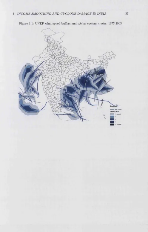
both raw data sets are displayed in Figure 1.1. The map, for example, clearly shows
th a t stronger cyclones are associated with both larger wind speed buffers and longer
cyclone tracks. I thus proxy for the size of the wind speed buffers by summing the
cyclone track length within a district. To capture possible non-linearities in this re
lationship, I square the track length variable and use it as an additional regressor in
the prediction. The other 14 variables are constructed similarly and explained in full
in Appendix A.3.
These 16 controls are subsequently regressed on the dependent variable constructed
7The data can be ordered at h ttp ://w w w .im d ch en n a i.g o v .in /cy clo n e_ ea tla s.h tm . Appendix A.3 contains additional information on this database.
8The dataset can be downloaded from h t t p ://p review .g rid .u n ep .ch /in d ex .p h p ? p rev iew = data&events=cyclones&lang=eng. More information on the data is provided in Appendix A.2.
9I use the district boundaries of 1966 throughout the analysis. This makes the cyclone data compatible with the World Bank’s India Agriculture and Climate dataset, which is my main source of data for the primary sector (see Section 1.3.3 for more detail).
1 INCO M E SM OOTHING AN D C YC LO N E DAM AGE IN IND IA 21
from the UNEP data. The latter measures the percentage of the district’s area covered
by a wind speed buffer for the period of overlap, 1977-200311. The dependent variable
is then predicted out of sample for 1891 to 2008. This yields the so-called cyclone
exposure variable, which will be the main control of interest in the empirical analysis.
Note th a t the standard errors will have to be bootstrapped in the regressions, since
the cyclone exposure variable is a predicted regressor. Finally, I have recorded the
date information for each of the 16 eAtlas controls. Therefore, I can determine when
a cyclone hits a given district, which will be im portant for the identification strategy
later on.
Nonetheless, there are two problems with using the eAtlas data for this prediction. Firstly, it codes storms with wind strength of 48 knots (equivalent to 88.9km/h) or
more as cyclones, whereas the UNEP d ata uses a much higher threshold of 96 knots
(177.8km/h). Since no wind speed measurements are available for the eAtlas, I cannot
distinguish weaker from stronger storms. Therefore, all of the cyclone events will have
to be included in the prediction. As a consequence, there is a risk of overpredicting exposure, especially at the low end of the distribution. I therefore construct a second
severe cyclone exposure variable, which restricts the prediction to being greater or
equal to 25% of the district’s territory.12
To assess the quality of these predictions, I first compare the dependent variable
with the cyclone exposure variable for the period of overlap. The correlation between these two variables is displayed in Figure 1.2a. It clearly shows th a t the eAtlas data
often predicts damage, when none was recorded by the UNEP wind speed buffers.
This leads to a Pearson’s correlation coefficient of 0.29. The coefficient increases to 0.44, if the correlation is only calculated for strictly positive values of the dependent
variable (Figure 1.2b), and to 0.46 for the severe cyclone exposure variable (Figure
1.2c). Similarly, Spearman’s rank correlation coefficient increases from 0.13 to 0.45 to
0.47 as the sample is restricted further.
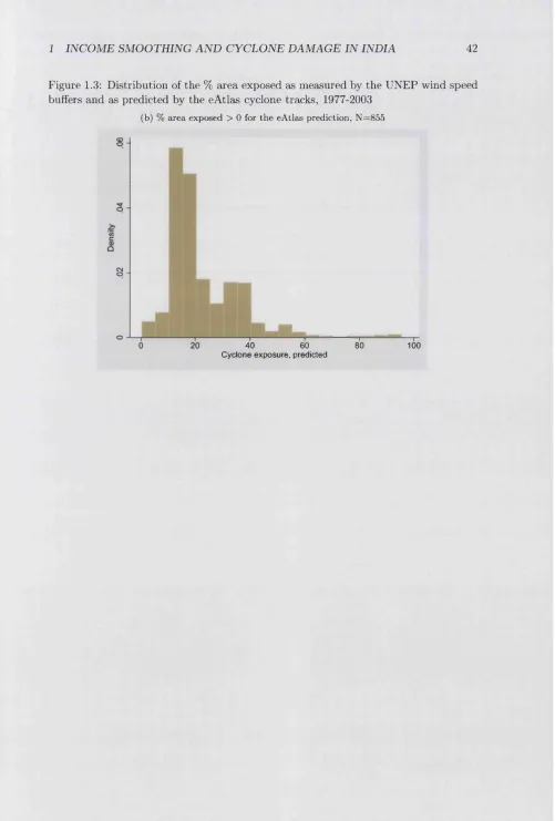
The improved fit can also be seen when comparing the distributions of the pre
dicted variables with the dependent variable for the period of overlap. Figure 1.3a
shows th a t the distribution of the UNEP data is twin-peaked with a large mass at very
low and high levels of the percent area affected. Thus, it has a large standard error of
3.44 around its mean of 33.46%. The distribution of the predicted cyclone exposure
variable is instead centred on its mean of 22.74% with a standard error of only 0.47
(Figure 1.3b). Yet, once the distribution is truncated for the severe cyclone exposure
variable (Figure 1.3c), it more closely resembles the UNEP data - it is then skewed
to the right and its mean and associated standard error almost double to 39.41% and
0.83 respectively.
These results seem to suggest th at the severe cyclone exposure variable better fits
1 INCO M E SM OOTHING A N D C YC LO N E DAM AGE IN IND IA 22
the UNEP d ata and should thus be used in the regression analysis. However, it is
im portant to note th a t the truncation considerably limits the number of district-level
cyclone events. For the final sample period ranging from 1956 to 1987, the number of
district-level cyclone events drops from 1138 to 273 through the restriction. This will
significantly lower the precision of the estimates in the empirical analysis. These two
factors will have to be weighed against each other before making a final decision on
which variable to use.
The second problem with the eAtlas d ata concerns measurement error. Firstly, I
need to use a much simpler model than the UNEP team to estimate the percentage
of the district’s area affected. Moreover, the eAtlas cyclone tracks only roughly follow
the movement of the UNEP wind speed buffers, which can be clearly seen in Figure
1.1. To address this issue, I construct a third variable, which solely relies on the
eAtlas data. More specifically, I simply calculate the district’s minimum distance to
the nearest cyclone track. However, this minim um distance variable only provides a
lower bound estimate of cyclone exposure, since its correlation with the UNEP wind
speed buffers is only 0.12 in absolute value as opposed to 0.44 for the cyclone exposure
variable. It will thus be used as a robustness check in the empirical analysis.
Table 1.1 displays the summary statistics for all three eAtlas-based cyclone vari ables for the sample period used in this analysis, 1956-1987. The data is reported for
all observations in Panel A and for the respective cyclone samples in Panel B. The
overall probability of being exposed to a cyclone is very low; on average only 2.37% of the district’s area is exposed to the cyclones as measured by the cyclone exposure
variable - a figure th a t drops to 1.05% for the severe cyclone exposure variable. Sim
ilarly, the minimum distance to the nearest cyclone is large on average at 775.40km.
However, if a district is struck by a cyclone, exposure increases dramatically to 21.41%
and 39.54% for the cyclone exposure and severe cyclone exposure variable respectively.
The average minimum distance to the nearest cyclone track also drops significantly
to 237.46km.
1.3.3 D a ta for th e prim ary sector
The outcome variables for this analysis were retrieved from the World Bank’s In
dia Agricultural and Climate D ataset (WB).13 This is a comprehensive district-level
database for the primary sector th a t provides production information on an annual ba
sis for 1956 to 1987 - note th at a year is defined as an agricultural year, which roughly
runs from April to the following March. The sample includes 271 districts within 13
states (which use the 1966 boundaries) covering almost 80% of the Indian territory.14
I only lack information on two agriculturally im portant states, namely Kerala and
Assam. Nonetheless, this is not a major concern for the current analysis, since both
13The data can be downloaded from h ttp ://ip l.e c o n .d u k e .e d u /d th o m a s/d e v _ d a ta /in d e x .h tm l. For more information on the dataset see Appendix A .4.
1 INCO M E SM OOTHING A N D C YCLO NE D AM AG E IN IND IA 23
states are not hit by a tropical cyclone during the sample period. Consequently, they
would have only contributed to the estimation of the fixed effects.
The great advantage of this dataset is th a t it contains crop-level information on
farm harvest prices, agricultural output, and area planted for each district. This data
is available for 6 major and 14 minor crops, which cover a wide variety ranging from
cereals to fibre crops.15 It also reports price and quantity information for variable
inputs, such as fertilizer, agricultural labourers, bullocks and tractors. Unfortunately,
this data is only available at the district level. This makes it impossible to calculate
crop-level profits or to analyse potential changes in the production technology in
response to the shock. Moreover, the labour and capital d ata is collected only in
decennial and quinquennial censuses respectively. Therefore, it fails to capture the
disaster impact, making it unsuitable for the present study.
Instead, the empirical analysis focuses on the crop-level variables measuring the
area planted, output and farm harvest prices. Note th a t I adjust prices with the
agricultural GDP deflator for 1980. I also construct three additional outcome vari
ables. First of all, I capture the value of production by calculating earnings as the product of prices and quantities. Secondly, to measure productivity, I compute yields
th a t are equal to the ratio of earnings to the area planted. Finally, I proxy for the nutritious value of the crops by converting the output d ata into its calorie content.
These calculations use weights obtained from MeDINDIA - a premier health portal
in India.16
Nonetheless, more information is needed to identify the impact of tropical cyclones
on the primary sector. The reason for this is th at cyclone events occur throughout the
agricultural year.17 These shocks thus have a differential effect across crops depending
on their position in the growing cycle. The situation is further complicated by the
fact th at most Indian districts have two and some even three growing seasons (GOI,
1967). Consequently, some crops within the same agricultural year are affected by the cyclone, whereas others are planted only after the shock. To disentangle these effects,
the WB dataset is augmented with a district-level crop calendar (GOI, 1967).18 This
growing season information allows me to distinguish which crops in my sample were
sown before or after a given cyclone shock.19
Section 1.4 now explains how this distinction helps identify the impact of tropical
15The six major crops are bajra, jowar, maize, rice, sugar, and wheat. The 14 minor crops are barley, cotton, gram, groundnut, jute, other pulses, potatoes, ragi, rapeseed and mustard, sesamum, soy, sunflowers, tobacco, and tur.
16The calorie information was downloaded on 22nd of July 2010 at h ttp://w w w .m ed in d ia.n et/ p a tie n t s /f o o d c a lo r ie s /in d e x .a s p
17For the cyclone exposure variable, storms occur from February-December, whereas for the severe cyclone exposure variable, shocks occur from April-December.
18 Appendix A.5 provides more information on the construction of this dataset.
1 INCO M E SM OOTHING A N D CYC LO NE DAM AGE IN IND IA 24
cyclones on agricultural production and crop mix choices.
1 .4 I d e n tific a tio n s t r a t e g y
1.4.1 M otivation
The identification strategy is built on the following two observations about tropical
cyclones. Firstly, the movement and intensity of each storm is solely determined by
climatic and oceanic conditions (IMD, 2009). The cyclone shock is therefore exogenous
to the primary sector allowing me to estimate its causal impact on agricultural output
and production choices. Note th a t this effect is heterogeneous across districts due
to the non-random movement of tropical cyclones. For example, in this dataset,
8.4% of all districts suffer one third of all cyclone shocks prior to 1956. We would
thus expect producers in these high-risk regions to anticipate the event and adjust their production behaviour accordingly. However, since they constitute such a small
fraction of the sample, the estimates are too imprecise to identify a differential effect.
I therefore restrict myself to estimating the average cost and behavioural response.
Secondly, tropical cyclones form throughout the year and can affect the same
district in different months.20 As has been explained in Section 1.3.3, the impact of the
shock thus differs across crops within the same agricultural year due to the presence
of multiple growing seasons. Specifically, some crops axe hit by the cyclone prior to their harvest. Their output is hence destroyed. However, there is a second group of
crops th a t has not been sown yet. Given th a t cyclone shocks axe largely uninsured, producers can thus respond in a variety of ways. For instance, they might intensify
their input use in the subsequent growing season to raise yields. Alternatively, farmers
could expand production by using land th at was supposed to be fallow21. They might
also plant more resilient crops such as coarse cereals th a t can flourish on marginal land
(Sawhney and Daji, 1961). These crops have the added advantage of a high calorie
content22, which will help farmers smooth both income and nutrition in the aftermath
of the natural disaster.
Given th a t producers can respond to the shock within the same year, a simple
regression of cyclone exposure on agricultural output will not estimate the total level
of destruction. Instead it will provide a measure of the net effect of a tropical cyclone.
T hat is, it will capture both the damage caused and the subsequent behavioural
response of the producers. These two effects counterbalance each other and it is not
20Cyclone shocks occur from February to December for the cyclone exposure and minimum distance
variables and from April to December for the severe cyclone exposure variable. However, the prime cyclone season runs from May until November, with more than three quarters of all shocks occurring during that time period for all three cyclone measures.
21 Summer and winter crops are often planted in rotation, which can include fallow periods. For example, the maximum production of barley can only be achieved if the land is not cropped in the preceding summer (Sawhney and Daji (1961), p. 116). The suitability of a given combination of crops depends on local climate, soil characteristics, and the availability of irrigation facilities.
1 INCO M E SM OOTHING AN D C YCLO NE D AM AG E IN IND IA 25
clear a priori which effect should outweigh the other. It is therefore an empirical
question to determine if the change in behaviour is sufficient to offset the impact
of the natural disaster. I can estimate this overall effect by regressing the cyclone
exposure variable on the production d ata for the entire universe of crops.
I can even take the analysis one step further and break up the overall effect into
its individual components. To do so, I exploit the interaction between the timing of
the cyclone shock and the multiple growing seasons in my sample. For example, I
distinguish between cyclones th at occurred before and after the sowing time of the
so-called winter crops - i.e., crops planted in the second half of the agricultural year. If
these two cyclone variables axe then regressed on the o utput of winter crops only, I can
separately identify the cyclone impact and coping strategy. T h at is, if the district was
hit by a cyclone at the beginning of the year, farmers should have smoothed income
by expanding production and thus output in the second growing season. However,
shocks th a t occurred towards the end of the year should have destroyed the standing
winter crops with no room for recovery. The converse argument can be applied to the
summer crops, where the destruction of the harvest in the previous year should have led to an increase in production in the next growing season.
Furthermore, I investigate if farmers change their crop mix towards coarse cereals
in response to the shock. As has been argued above, producers might choose to
plant more coarse cereals after a cyclone shock to ensure a steady income and cheap
calories. However, by doing so farmers forgo higher income. T hat is, coarse cereals are generally of low economic value - on average, they fetch prices half the size of other
food crops in my sample. Therefore, we would expect this change in the crop mix
to be only temporarily. I can test for this coping strategy by splitting the data into
coarse cereals23 and all other food crops24. I then estimate the net effect of cyclone
exposure for both groups separately and test for the persistence of the shock. Section 1.4.2 now describes how this identification strategy is implemented.
1.4.2 Em pirical Im plem en tation
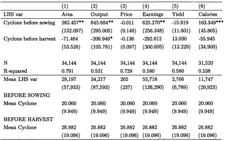
Firstly, I estimate the net effect of tropical cyclone on agricultural production with
an OLS fixed effects regression, as follows:
Vcdt = « +
P
cyclonedt + \ d+ Vc+
I t+
tc d t,
(!)
where y ^ t is either the area planted, output, farm harvest price, earnings, yields,
or calorie content of crop c in district d in year t, and cyclonedt is one of the three
district-level cyclone exposure variables discussed in Section 1.3.2. The coefficient /?
23The following crops are included in the coarse cereal category: bajra, barley, gram, jowar, and ragi.
1 INCO M E SM OOTHING A N D C YC LO N E D AM AG E IN INDIA 26
thus captures the net causal impact of cyclone damage on agricultural production and
crop mix choices. The regression also controls for time-invariant crop and district
fixed effects, A^ and p c respectively.25 In addition, 7* controls for common macro
shocks26, because agricultural policy is set by the central government. Given th a t the
c y c lo n e e x p o su re variables are predicted regressors, the standard errors are clustered
at the district level and bootstrapped. Lastly, the regression is weighted by the share
in initial production of crop c in district d, since there is substantial variation in
output across crops and districts - the 5th percentile of the output variable is 44 tons,
whereas the 95th percentile is 150,800 tons.27
To investigate the dynamics of cyclone’s net impact, I simply include three lags of
the cyclone exposure variable into equation (1):
Vcdt = a + f t o c y c lo n e dt + 0 n c y c l o n e ^ ^ + 0 i 2 c y c lo n e dt_ 2 + 0 i 3 c y c lo n e dt_ 3
(2) + Ad + /xc + 7* + ecdt
The results are robust to the inclusion of more lags. Since the effects generally lose
significance with the second or third lag, I focus the analysis on this specification.
On the one hand, we would predict th a t the coefficients on the lags are statistically
significantly different from zero, as producers take tim e to recover from the shock. Yet, these coefficients should lose significance over time, as the empirical literature on
large temporary shocks does not find lasting changes in production behaviour (Davis
and Weinstein, 2002; Miguel and Roland, 2006).28
Furthermore, I can carry out a falsification exercise to verify th at I am indeed
capturing the impact of an exogenously determined natural disaster. Specifically, I
include three leads of the cyclone exposure variable into regression (2). Their coef
ficients should be jointly insignificantly different from zero, if I am indeed capturing
the impact of an exogenously determined natural disaster. T hat is, there should be
no pre-trends in the data th at are captured by the cyclone variable after controlling
for common macro shocks.
Secondly, I disentangle the direct impact of the cyclone on agricultural production
from the subsequent behavioural response of the producers to shock. To do this,
25The inclusion of crop-by-district fixed effects does not change the results substantially. This is not surprising, as each crop category comprises several varieties, which the dataset does not distinguish separately (Sawhney and Daji, 1961). Thus, there should not be much variation in the observed
suitability of one crop across districts, as farmers have already chosen the optimal variety. Moreover, districts are small geographical units, so that most of the variation is absorbed by Ad.
26The results are robust to the inclusion of crop-by-year fixed effects. This finding makes intuitive sense, as it is a well-known fact that markets are not well-integrated in India (Topalova, 2004; Duflo and Pande, 2007; Guiteras, 2007). In fact, my results below show that farm harvest prices do respond to local shocks. Hence, it is unlikely that crop-level shocks equally affect all districts within India.
27This weight is calculated as the share in total production of crop c in district d for 1956-1958. If the crop was not produced during this time period the output level in the first year that it was planted is used for the calculation of the share.
1 INCO M E SM OOTHING A N D CYC