D im en sio n al T im e Series
LSE
Neil B athia
D epartm ent of Statistics
London School of Economics
A thesis subm itted for the degree of
Doctor of Philosophy
UMI Number: U615B02
All rights reserved
INFORMATION TO ALL U SE R S
The quality of this reproduction is d ep en d en t upon the quality of the copy subm itted.
In the unlikely even t that the author did not sen d a com plete m anuscript
and there are m issing p a g e s, th e se will be noted. Also, if material had to be rem oved, a note will indicate the deletion.
Dissertation Publishing
UMI U615B02
Published by ProQ uest LLC 2014. Copyright in the Dissertation held by the Author. Microform Edition © ProQ uest LLC.
All rights reserved. This work is protected against unauthorized copying under Title 17, United S ta tes C ode.
ProQ uest LLC
^ 4
© 2010 Neil Bathia
A cknow ledgem ents
Firstly, I would like to say that this thesis is not a result of my efforts alone. My advisor, Professor Qiwei Yao, provided me with immense guidance and support with seemingly infinite patience. A student could not wish for a more caring advisor. I will forever be in his intellectual debt.
I would also like to thank all of the staff and students in the LSE Statistics department for making the last three years one of the most memorable experiences of my life. In particular, I am indebted to all of the members of the of the Center for the Analysis of Time Series for their hospitality and countless stimulating discussions. Dr Flavio Ziegelmann is also due a special mention for his assistance with some of the computations in this thesis.
I am incredibly fortunate to have such amazing friends and family, without whose encouragement none of this would have been possible. I owe a great deal to my grandparents for the tremendous role they have played in my upbringing. In particular, my late grandfather Babulal strived to ensure that every dream I had was made a reality. I wish that he was here to celebrate this day with me. My uncle and aunt, Ajit and Nayna, have been like second parents to me and I hope that one day I will be able to repay them for their endless love and support. Also, my life would not be the same without my brothers and sisters, Raj, Krishma, Priyankaa and Nishal, who never fail to bring a smile to my face.
A b stract
Chapter 1: Identifying th e finite dim ensionality of curve
tim e series
The curve time series framework provides a convenient vehicle to model some types of nonstationary time series in a stationary frame work. We propose a new method to identify the finite dimensionality of curve time series based on the autocorrelation between different curves. Based upon the duality relation between row and column subspaces of a data matrix, we show that the practical implementa tion of our methodology reduces to the eigenanalysis of a real matrix. Furthermore, the determination of the dimensionality is equivalent to indentifying the number of non-zero eigenvalues of this same ma trix. For this purpose we propose a simple bootstrap test. Asymp totic properties of our methodology are investigated. The proposed methodology is illustrated with some simulation studies as well as an application to IBM intraday return densities.
Chapter 2: M ethodology and convergence rates for factor
m odeling o f m ultiple tim e series
results suggest that the sample eigenvalues whose population counter parts are zero are “super-consistent” (i.e. they converge to zero at a n
rate) whereas the sample eigenvalues whose population counterparts are non-zero converge at an ordinary parametric rate of root-n. Here
1 Identifying th e finite dim ensionality o f curve tim e series 1
1.1 In troduction ... 1
1.2 Methodology ... 4
1.2.1 Characterization of dand M via serial dependence... 4
1.2.2 Estimation of dand JVC... 7
1.2.2.1 Estimators and fitted dynamic m o d e ls ... 7
1.2.2.2 E igenanalysis... 7
1.2.2.3 Determination of dvia statistical t e s t s ... 9.
1.3 Theoretical properties ... 10
1.4 Numerical p ro p e rtie s ... 13
1.4.1 S im u la tio n s... 13
1.4.2 Intraday return d e n sitie s... 17
1.5 D iscussion... 25
1.6 P r o o f s ... 26
2 M ethodology and convergence rates for factor m odeling o f mul tiple tim e series 33 2.1 In troduction ... 33
2.2 Methodology ... 35
2.2.1 Factor m o d e ls... 35
2.2.2 Estimation of JVC ... 36
2.2.3 White noise test for d... 37
2.2.4 Modeling via common f a c t o r s ... 39
2.3 Theoretical results ... 40
C O N TEN TS
2.5 Implied volatility s u r f a c e s ... 54
2.5.1 Data description ... 54
2.5.2 Estimation results... 55
2.6 P r o o f s ... 62
A Background on operator theory 71
B Some useful technical Lemma’s 73
Id en tifyin g th e finite
d im en sionality o f curve tim e
series
1.1
In trod u ction
A curve time series may consist of, for example, annual weather record charts, annual production charts or daily volatility curves (from morning to evening). In these examples the curves are segments of a single long time series. One advantage to view them as a curve series is to accommodate some nonstationary features (such as seasonal cycles or diurnal volatility patterns) into a stationary framework in a Hilbert space. There are other types of curve series th at cannot be pieced together into a single long time series; for example, daily mean-variance efficient frontiers of portfolios, yield curves and intraday asset return distributions. The goal of this chapter is to identify the finite dimensionality of curve time series in the sense th at the serial dependence across different curves is driven by a finite number of scalar components. Therefore the problem of modeling curve dynamics is reduced to that of modeling a finite-dimensional vector time series.
1.1 Introduction
to errors in the sense that
Yt(u) = X t(u) + et {u), u e l , (1.1)
where X t(-) is the curve process of interest. The existence of the noise term e(-) reflects the fact that curves X t (-) are seldom perfectly observed. They are often only recorded on discrete grids and are subject to both experimental error and numerical rounding. These noisy discrete data are smoothed to yield the ‘observed’ curves Yt (-). Note that both X t(-) and et(-) in (1.1) are unobservable.
We assume that £*(•) is a white noise sequence in the sense that E {et{u)} = 0 for all t and Cov{£t(u ),ss(v)} = 0 for any u ,v G 3 as long as t ^ s. This is guaranteed since we may include all of the dynamic parts of Yt(-) into X t (-).
Likewise, we may also assume that no parts of X t(') are white noise since these parts should be absorbed into £*(•)• We also assume that
J B { X t (u)2 + et{ u f} d u < oo, (1.2)
and both
= E { X t(u)}, M k(u,v) = Cov { X t(u ),X t+k(v)} (1.3)
do not depend on t. Furthermore, we assume th at X t (-) and st+k{-) are uncorre lated for all integer k. Under condition (1.2), ^t(-) admits the Karhunen-Loeve expansion
oo
X t{u) - n(u) = (1.4)
j=i
where £tj = — fi(u)}(pj(u)du are a sequence of scalar random variables with E(gtj) = 0, Var(fy) = Aj and C o v (^ ,^ j) = 0 if i =tj. We rank {^tj, j > 1 }
such th at Xj is monotonically decreasing as j increases.
We say that X t{-) is d-dimensional if A^ ^ 0 and A^+i = 0, where d > 1 is a finite integer; see Hall h Vial (2006). The primary goal of this chapter is to identify d and to estimate the dynamic space JVC spanned by the (deterministic)
terms as one cannot separate X t(-) from £*(•) in (1.1). This difficulty was resolved in Hall & Vial (2006) under a ‘low noise’ setting which assumes that the noise £*(•) goes to zero as the sample size goes to infinity. This condition is reasonable under an infill asymptotic scheme, i.e. when the observations on each curve are relatively dense. However, when dealing with a sparse design the condition is far from adequate and penalties are incurred in terms of the convergence rates of the resulting estimators; see Hall et al. (2006). Our approach is different and it does not require the low noise condition, since we identify d and JVC in terms of the serial dependence of the curves. Our method relies on a simple fact that Mfc(u, v) = Cov{y*(u), Yt+k(v)} for any k ^ 0, which automatically filters out the noise see (1.3). In this sense, the existence of dynamic dependence across different curves makes the problem tractable without the low noise argument.
Dimension reduction plays an important role in functional data analysis. The most frequently used method is functional principal component analysis in the form of computing the spectral decomposition of the empirical covariance opera tor. The literature in this field is vast and dates back to the early work of Besse & Ramsay (1986), Dauxois et al. (1982), Ramsay &; Dalzell (1991) and Rice & Silverman (1991). Much of the work is described in Ramsay & Silverman (2005). However, despite the methodological advancements in functional data analysis with independent observations, the work on functional time series has been of a more theoretical nature; see e.g. Bosq (2000). The available inference methods focus mostly on nonparametric estimation of some characteristics of functional series (Part IV of Ferraty & Vieu (2006)). As far as we are aware, this work represents the first attempt on the dimension reduction based on dynamic de pendence. Although we confine ourselves to square integrable curve series in this chapter, the methodology may be extended to a more general functional frame work including, for example, a surface series which is particularly important for environmental studies; see Guillas & Lai (2008).
1.2 M ethodology
eigenfunctions in a functional space directly. The theoretical results of the esti mation are presented in Section 1.3. Numerical illustration using both simulated and real datasets is provided in Section 1.4 and Section 1.5 closes with a brief discussion. We relegate all of the technical proofs to Section 1.6.
1.2
M eth o d o lo g y
1.2.1 C h a ra cteriza tio n o f
d
and 3VC v ia serial d ep en d en ce
Let £/2p ) denote the Hilbert space consisting of all square integrable curves de fined on J equipped with the inner product
( f , 9 ) = J f ( u ) g { u ) d u, f , g G C 2(J). (1.5)
Now Mk defined in (1.3) may be viewed as the kernel of a linear operator acting on £2p), i.e. for any g £ £ 2(3), Mk maps g(u) to g(u) = J0M k(u:v)g(v)dv. For
notational economy, we will use Mk to denote both the kernel and the opera tor. Some relevant facts about operators acting on Hilbert spaces are listed in Appendix A.
For Mo defined in (1.3), we have a spectral decomposition of the form
00
Mo(u, v) = ^ Xjipj(u)ipj(v), u , u £ j , (1.6)
j= 1
where Ai > A2 > • • • > 0 are its eigenvalues and </?i, (p2, • • • are the corresponding orthonormal eigenfunctions (((/?*, tpj) = 1 for i = j, and 0 otherwise), i.e.
/
Mo(u,v)ipj(v)dv = A j > 1.Furthermore the random curves Xt(•) admit the representation (1.4). We assume in this chapter th at X t(-) is d-dimensional (i.e. A^+i = 0). Therefore
d d
Mo(u, v) = ^ 2 \ j ‘pj {u)ipj (v), X t{u) = n(u) + Y^€tj<Pj(u). (1.7)
It follows from (1.1) that
d
Yt(u) = n(u) + ^2StjV iM + £<(“ )- f1-8)
j=i
Hence the serial dependence of Ff(-) is entirely determined by that of the
d-vector process £t = (£ti, • • • ,€td)' since £*(•) is white noise. By the virtue of the Karhunen-Loeve decomposition E ( £ t) = 0 and Var(£t) = diag(Ai, • • • , A<*).
Denote our estimator of Mk in (1.3) by
n - p
Mk(u,v) = —— 5 ] { ^ ( U) - ? ( « ) } { l 5 + i(« )- ? ( « ) } , (1.9)
" p=ij
where y(-) = n~l 5Zi<j<n an<^ P > 1 is a prescribed integer. The reason for truncating the sums in (1.9) at n — p as opposed to n — k is to ensure a duality operation which simplifies the computation of the eigenfunctions; see Remark 2.2 at the end of Section 1.2.2.2. The conventional approach to estimate d and M = span{</?i(-), • • • pd(-)} is to perform an eigenanalysis on M0 and let d be the number of non-zero eigenvalues and M be spanned by the d corresponding eigen functions; see for example, Ramsay & Silverman (2005) and references therein. However this approach suffers from complications due to fact that Mo is not a con sistent estimator for Mo since Cov{Yt(u), Vt(w)} = Mo(u, v) + Cov{et (u), et(v)}.
Therefore Mo needs to be adjusted to remove the part due to et(•) before the eigenanalysis may be performed which is a non-trivial matter. An alternative is to let the variance of et(-) decay to zero as the sample size n goes to infinity; see Hall & Vial (2006).
We adopt a different approach based on the fact that Cov{y4(ii), Yt+k{v)} =
M k(u,v) for any k ^ 0, which ensures that Mk is a legitimate estimator for Mk;
see (1.3) and (1.9).
Let = E(€t€'t+k) = (aij^) ke the autocovariance matrix of £t at lag k. It
1.2 M e th o d o lo g y
where = {w ff) = is a non-negative definite matrix. Then it holds for any integer k that
J
N k(u,v)((v)dv = 0, for any £(•) G JVCJ_, (1-H)where M-1 denotes the orthogonal complement of M in /C2P). Note (1.11) also holds if we replace N k by the operator
v
K ( u , v ) = y ^ N k( u, v) (1.12)
fc=i
which is also a non-negative operator on .C2P).
P ro p o sitio n 1.1 Let the matrix Hk be full-ranked for some k > 1. Then the assertions below hold.
(i) The operator Nk has exactly d non-zero eigenvalues, and JVC is the linear
space spanned by the corresponding d eigenfunctions. (ii) For p > k, (i) also holds for the operator K.
R em ark 1.1 (i) The condition that rank(Efc) = d for some k > 1 is implied by the assumption that Yt(-) is d-dimensional. In the case where rank(Sjt) < d. for all k, the component with no serial correlations in X t(-) should be absorbed into the white noise term £*(•); see similar arguments on modeling vector time series in Pena & Box (1987) and Pan & Yao (2008).
(ii) The introduction of the operator K in (1.12) is to pull together the infor mation at different lags. Using a single Nk may lead to spurious choices of d; see Section 1.2.2.3
(iii) Note that f 3K(u, v)Q{v)dv = 0 if and only if f 0 Nk(u, v)£(v)dv = 0 for all
1 < k < p. However, we cannot use Mk directly in defining K since it does not
1.2.2
E stim ation o f
d
and M
1.2.2.1 E stim ato rs and fitted dynam ic m odels
As we have stated above, Mk for k ^ 0 may be directly estimated from the observed curves Yt\ see (1.9). Hence a natural estimator of K may be defined as
K (u,v) = Y
k= 1
=
E EW(«) -
-
y
),
' t,s= 1 fc=l
see (1.12), (1.10), (1.9) and (1.5).
By Proposition 1.1 we define d to be the number of non-zero eigenvalues of K (see Section 1.2.2.3 below) and M to be the linear space spanned by the
d corresponding orthonormal eigenfunctions tpi( ■ ) > • * ' This leads to the fitting
d
Yt(u) = Y (u) + Y u e 3 , (1.14)
3 = 1
where
% = f { Y t{ u )-Y { u )} ^ j(u )d u r j = l,--- ,d. (1.15)
See (1.8). Although M = span{^i(-)5 • • • is a consistent estimator for M = span{</?i(-), • • • , (Theorem 1.2 in Section 1.3 below), -ipj are the esti mators for the eigenfunctions of K defined in (1.12), which are different from the eigenfunctions <fj of M0 defined in (1.6). Therefore rjt = (rfti, • • • ,rjt^)' is not an estimator for £t used in (1.8).
Now in order to model the dynamic behavior of Vf(-), we only need to model the d-dimensional vector process rjt which may be done using VARMA or any other multivariate time series models. See also Tiao & Tsay (1989) for applying linear transformations in order to obtain a more parsimonious model for rjt.
1.2.2.2 Eigenanalysis
To perform an eigenanalysis in a Hilbert space is not a trivial matter. A popular pragmatic approach is to use an approximation via discretization, i.e. to evaluate
1.2 M e th o d o lo g y
the observed curves at a fine grid and consequently replace them with the resulting vectors. This effectively transforms the problem to the eigenanalysis of a finite matrix. See, e.g. Section 8.4 of Ramsay & Silverman (2005). Below we also transform the problem into the eigenanalysis of a finite matrix but not via any approximations. Instead we make use of the well-known duality property that A B ' and B'A share the same non-zero eigenvalues for any matrices A and B of the same sizes. Furthermore if 7 is an eigenvector of B'A, A 7 is an eigenvector of A B ' with the same eigenvalue. In fact this duality also holds for operators acting on function spaces. This scheme was adopted in Kneip & Utikal (2001) and Benko et al. (2009) but the adaptation to our setting is more involved so we provide a detailed exposition.
We present a heuristic argument first. To view the operator K(•, •) defined in (1.13) in the form of AB', let us denote the curve V^(-) — V" (*) a s a n o o x l vector Y t with Y ;Y s = {Yt — Y ,Y S - Y); see (1.5). Put y k = (Y 1+fc, • • ■ , Y n_p+fe). Then K(-, •) may be represented as an 00 x x matrix
Applying the duality stated the above with A = y0 and B' = K
shares the same non-zero eigenvalues with the (n — p) x (n — p) matrix
(1.16)
where the (£, s)-th element of y'ky k is Y't+kY s+k = (Yl+k - Ys+k - Y ) and
k = 1, ••• ,p. Furthermore, let 7 ^ = (7^ , • •• ,7n- p,j)', j = 1, ••• ,d, be the eigenvectors of K* corresponding to the d largest eigenvalues. Then
' E ' l t A Y t ( - ) - ? ( ■ ) } , (1.17)
t= 1
are the d eigenfunctions of K(-, •). In practice, it is likely that the functions in (1.17) may not be exactly orthogonal. Thus the orthonormal eigenfunctions
This heuristic argument is justified by the result below. The formal proof is relegated to Section 1.6.
P ro p o sitio n 1.2 The operator •) shares the same non-zero eigenvalues with
matrixK* defined in (1.16) with the corresponding eigenfunctions given in (1.17).
R e m a rk 1.2 The truncation of the sums in (1.9) at (n — p) for different k
is necessary to ensure the applicability of the above duality operation. If we truncated the sum for Mk at (n — k) instead, would be of different sizes for different A;, and K* in (1.16) would not be well-defined.
1.2.2.3 D e te rm in a tio n o f d v ia s ta tis tic a l te s ts
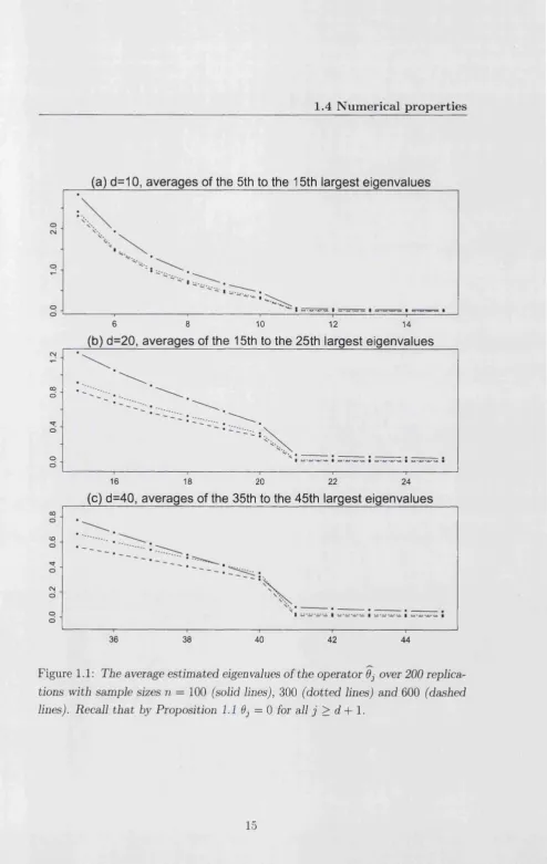
Although the number of nonzero eigenvalues of the operator K(-, •) defined in (1.12) is d (see Proposition 1.1), the number of nonzero eigenvalues of its es timator K{-, •) defined in (1.13) may be much greater than d due to random fluctuation in the sample. One empirical approach is to take d to be the number of ‘large’ eigenvalues of K in the sense that the (d+ l)-th largest eigenvalue drops significantly; see Figure 1.1. A more formal method of determining the value of
d is given in the bootstrap test below.
Let 6\ > 02 > • • • > 0 be the eigenvalues of K . Suppose we are interested in
testing the null hypothesis
Hq . Odo+i 0)
where dois a known integer, obtained, for example, by visual observation of the
estimated eigenvalues 6\ > O2 > •• • > 0 of K . Hence we reject Ho if 0do+i > la,
where la is the critical value at the a E (0,1) significance level. To evaluate the critical value la,we propose the following bootstrap procedure.
1. Let Yt (') be defined as in (1.14) with d = do. Let £*(•) = Yt(-) — Yt(').
2. Generate a bootstrap sample from the model
!?(•) = « (•) + <£(•).
1.3 T h e o re tic a l p ro p e rtie s
3. Form the operator K* in the same manner as K with {!*} replaced by {Yt*} and compute the (do + l)-th largest eigenvalue 0 ^ +1 of K*.
Then the conditional distribution of 0JO+1, given the observations {Yi, • • • , Yn}, is taken as the distribution of 6^ + i under Ho- In practical implementation, we repeat steps 1 and 2 above B times for some large integer B, and we reject H0
if the event that 0 ^ +1 > 6^ + i occurs no more than [aB] times. The simulation results reported in Section 1.4.1 below indicate that the above bootstrap method works well. A full theoretical justification of the bootstrap is beyond the scope of this current work.
1.3
T h e o r e tic a l p r o p er tie s
We introduce some regularity conditions for model (1.8) first.
Cl. {!«(•)} is strictly stationary and satisfies the condition E[{J3 Yt(u)2du}2+S] <
oo for some 8 > 0.
C2. For p given in (1.12), the sequence {>*(•),..., Yt+P(-)} is strongly mixing in the sense that a(m) — * 0 a sm — * oo, where
a ( m ) = sup sup \P{U n V) - P (U )P (V) \ ,
i>i ue?
and = a{ Yj(-),. . . , Vj+P(-)}. In addition, it holds that J j j l i a (j)s^ 2+s^ <
oo with 8 given in Cl above.
C3. Cov { X s(u),£t(v)} = 0 for all s, t and u, v E J.
C4. The d non-zero eigenvalues of K defined in (1.12) satisfy 0i > • • • > Od > Q, i.e. they are all unique.
Karhunen-Loeve expansion of Xt(•) in (1.4) (with an analogous representation readily available for £«(•))> we may think of the mixing condition on the random function y*(-) as being equivalent to placing mixing conditions on it’s (scalar) Karhunen-Loeve coefficients.
(ii) We note that conditions Cl and C2 are in fact stronger than required (see Merlevede et al. (1997)). However, the necessary and sufficient conditions in this context would be messy and perhaps unintuitive so we have stated only a set of sufficient conditions here.
(iii) The condition that all eigenvalues of K are different ensures that its eigenfunctions are identifiable. It is still possible to obtain a form of consistency of the empirical eigenfunctions without this assumption but the proofs become a lot more technical and little further insight is to be gained.
We now solidify some notation before presenting the asymptotic results. De note by and (Oj,ipj) the (eigenvalue, eigenfunction) pairs of K and K
respectively (see (1.12) and (1.13)). We will always arrange the eigenvalues in descending order, i.e. Bj > Bj+i and Bj > Bj+1- As the eigenfunction of K and K
are only unique up to sign changes, in the sequel it will go without saying that the right versions are used. Finally, for any operator L acting on £ 2(J), denote by ||jL|[x the sum of the absolute eigenvalues of L; see also Appendix A. All of the results in this section require that p is a fixed and finite integer.
T h eo rem 1.1 Let conditions Cl - C3 hold. Then as n —► oo, it holds that
\\K — K\\jj = Op(n~J/2) ands u p ^ |Bj — Bj| = Op(n~_1/2). In addition, if C4 also holds, then
Note that the results of Theorem 1 hold even if d = oo, i.e. when the dynamic space M is infinite dimensional.
1.2.2.1.) To measure the error in estimating M by 3VC, we introduce a measure for the discrepancy of any two d-dimensional subspaces Ni and N2 in £ 2(J). Let
1 < j < d .
1.3 Theoretical properties
{ C i i (* ))' ’ ’ >Cid(')} be an orthonormal basis of N*, i = 1, 2. Then the projection
of Cifc onto !N2 may be expressed as
d
It is clear that this is a symmetric measure between 0 and 1. It is independent
and only if Ni = 3Sf2. Let Z be the set consisting of all d-dimensional subspaces of £ 2p ). Then (Z, D) forms a metric space in the sense that D is a well defined distance measure on Z (see Lemma 1.4 in Section 1.6 below).
We are now in a position to state consistency results about M. We also consider the asymptotic properties of M = span{-0 i , . . . , ■0^} where d is some estimator of d. Since d may differ from d, we use a modified version of D (D'
given in (1.19)) to measure the distance between M and M.
T h e o re m 1.2 Let conditions Cl - C4 hold. In addition, suppose that the condi tions of Proposition 1.1 are satisfied and d is fixed, finite and known, (i) Then as n —> oo, it holds that D(3Vf, M) = Op(n~1^2) ■ (H) In addition if d d, then it
holds that - D(M ,M )| = o ^ n " 1/2).
A remarkable feature of Theorem 1.2 is the adaptivity property, i.e. we do not suffer any penalty in our estimation of M when dis unknown provided that it can be estimated consistently. Thus it is reasonable to assume that dis known when considering the asymptotic properties of our estimation of M. As remarked earlier, it is beyond the scope of this current work to provide a full theoretical justification of the bootstrap method for determining dgiven in Section 1.2.2.3.
} ^
(C2j>Clfc)C2j(^)-j=1
Its squared norm is 2 j L i ( ( C 2 j 5 Cifc))2 < 1- The discrepancy measure is defined as
(1.18)
1.4
N u m e r ic a l p ro p ertie s
1.4.1 S im u lation s
We illustrate the proposed method simulating data generated from model (1.1) with
d 100 g
x <(“ ) = e<(“ ) = e [o, i.],
i=l j=1
where { ^ , t > 1} is a linear AR(1) process with the coefficient (—l)l(0.9—0.5i/d), the innovations Z tj are independent N (0, 1) variables and
<Pi(u) = v/2cos(7riu), (j(u) = \/2sin(7rju).
We set the sample size to be n = 100, 300 or 600, and the dimension parameter d = 10, 20 or 40. For each setting we repeated the simulation 200 times. We used
p = 5 in defining the operator K in (1.13) and for each of the 200 simulations, we replicated the bootstrap method 200 times. Note that for this simulation experiment, the conditions of Proposition 1.1 are satisfied even if p = 1 so by taking p > 1 in constructing K we are accumulating estimation error. However, when analyzing a real dataset we would not know whether or not such a small value of p would be sufficient so taking p = 1 may lead to a spurious choice of d. Thus our aim in taking a value of p that is larger than necessary is to demonstrate that the methodology still performs well even when this is the case.
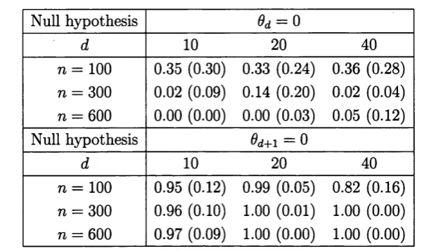
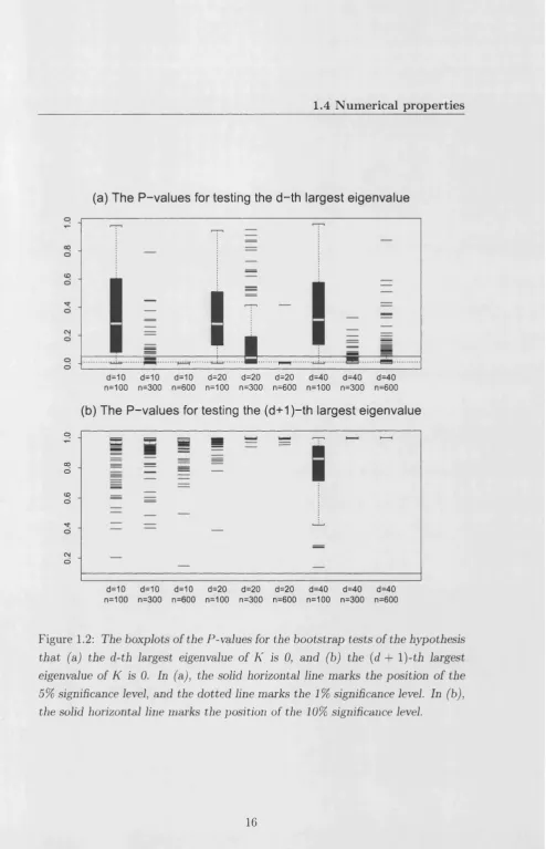
The average of the ordered eigenvalues of K obtained from the 200 replica tions are plotted in Figure 1.1. For better illustration, we only plotted eleven eigenvalues (i.e. five on the each side of the d-th largest eigenvalue). It is clear that drop from the d-th largest eigenvalue to the (d + l)-st is very pronounced. We applied the bootstrap method to test the hypothesis that the d-th or the (d + l)-st largest eigenvalue of K (0d and Oj+i respectively) are 0. The results are summarized in Table 1.1 and Figure 1.2. The bootstrap test could not reject the true null hypothesis 6d+\ = 0. In fact among the 200 replications for all the settings, the P-value was invariably greater than 10%; see panel (b) of Figure 1.2. The false null hypothesis 9d = 0 was routinely rejected by the bootstrap when
1.4 Num erical properties
Null hypothesis
d 10 20 40
n = 100
n = 300
n — 600
0.35 (0.30) 0.02 (0.09) 0.00 (0.00)
0.33 (0.24) 0.14 (0.20) 0.00 (0.03)
0.36 (0.28) 0.02 (0.04) 0.05 (0.12)
Null hypothesis @d+1 — 0
d 10 20 40
n = 100
n = 300
n = 600
0.95 (0.12) 0.96 (0.10) 0.97 (0.09)
0.99 (0.05) 1.00 (0.01) 1.00 (0.00)
0.82 (0.16) 1.00 (0.00) 1.00 (0.00)
Table 1.1: The means and standard deviations (in parentheses) o f the P-values of the bootstrap test.
To measure the accuracy of our estimation of the factor loading space M, we need to modify the metric D defined in (1.18) as dmay be different from d. Let Ni, N2 be two subspaces of <C2(J) with dimension d\ and d2respectively. Let {Ciij • • • , Qdi} be an orthonormal basis of Ni, i = 1,2. The discrepancy measure between the two subspaces is defined as
D '(X l 5N2) =
\
d\ d,2
It can be shown that Df(Ni , N2) G [0, 1]. It equals 0 if and only if Ni = N2, and 1 if and only if Ni flN 2 = 0. Obviously D'^Ni, N2) = D(Ni, 3\f2) when d\ = d2 = d.
[image:24.595.84.386.157.336.2](a) d = 1 0 , a v e r a g e s of the 5th to the 15th la rg est e ig e n v a lu e s
---1---i
i---1---1---6 8 10 12 14
(b) d = 2 0 , a v e r a g e s of the 15th to the 25th la rg est e ig e n v a lu e s
CM
CO
O
o
o
d
16 18 20 22 24
(c) d = 4 0 , a v e r a g e s of the 35th to the 45th la rg est e ig e n v a lu e s
CO
CM
d
o
o
36 38 40 42 44
Figure 1.1: The average estimated eigenvalues of the operator 6j over 200 replica
tions with sample sizes n = 100 (solid lines), 300 (dotted lines) and 600 (dashed
[image:25.597.28.523.26.808.2]1.4 N u m e ric a l p ro p e rtie s
(a) T h e P - v a lu e s for testin g th e d -th la rg est e ig e n v a lu e
i
i =
d=10 d=10 d=10 d=20 d=20 d=20 d=40 d=40 d=40 n=100 n=300 n=600 n=100 n=300 n=600 n=100 n=300 n=600
(b) T h e P - v a lu e s for testin g the (d + 1 )-th la rg e st e ig e n v a lu e
o
oo d
CD
d
•M -d
CM
d
d=10 d=10 d=10 d=20 d=20 d=20 d=40 d=40 d=40 n=100 n=300 n=600 n=100 n=300 n=600 n=100 n=300 n=600
Figure 1.2: The boxplots of the P-values for the bootstrap tests of the hypothesis
that (a) the d-th largest eigenvalue of K is 0, and (b) the (d + l)-th largest
eigenvalue of K is 0. In (a), the solid horizontal line marks the position of the 5% significance level, and the dotted line marks the 1% significance level. In (b), the solid horizontal line marks the position of the 10% significance level.
[image:26.595.27.522.27.795.2]d=10 d=20 d=40 o o o oo o o CD O d
n=100 n=300 n=600
o CN O O o CD o o
s
dn=100 n=300 n=600 oo o CO o o o o o 00 o o
s
o n=100 n=300 n=600
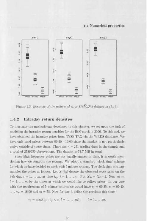
Figure 1.3: Boxplots of the estimated error ) defined in (1.19).
1.4.2
Intraday return d en sities
To illustrate the methodology developed in this chapter, we set upon the task of modeling the intraday return densities for the IBM stock in 2006. To this end, we have obtained the intraday prices from NYSE TAQ via the WRDS database. We have only used prices between 09:30 - 16:00 since the market is not particularly active outside of these times. There are n = 251 trading days in the sample and a total of 2786650 observations. The dataset is 73.7 MB in total.
Since high frequency prices are not equally spaced in time, it is w orth men
tioning how we com pute th e returns. We adopt a stan dard ‘clock tim e’ scheme
for which we have decided to work w ith 5 minute returns. The clock tim e strategy
samples the prices as follows. Let Xi(Uj) denote the observed stock price on the
«-th day, i = 1 , . . . , n, a t tim e j = 1 , . . . , n*. P u t X i0 = Xi(t n). Now let 77,
I = 1 , . . . , m be the tim es at which we would like to collect prices. In our case
w ith the requirem ent of 5 minute returns we would have T \ = 09:35, T2 = 09:40,
• • • ? Tm = 16:00 and m = 78. Now for day i, define the previous tick time
[image:27.595.28.523.36.781.2]1.4 N um erical properties
Let Xu = Xi(ru)- Then the Z-th return on day i is given by Zu — lo g p ^ /A ^ - i) ,
I = 1,.. . ,m. Note that sampling at 5 minutes in clock time for this dataset yields a total of n x m = 19578 effective observations.
One may also sample the prices based on some activity based scheme. For example, rather than sampling the prices every few minutes, an alternative may be to perform the sampling every few ticks. This type of strategy is known as sampling in ‘business time’. We performed the analysis using the business time sampling strategy as well but we have not reported the results here since they were very similar to the clock time based method.
Now given a set of high frequency returns, we estimate the intraday return densities by using a simple kernel density estimator
Yt (u) = (nht) - ' ^ K ( ? ± ^ y t = (1.20)
where K (u) = ( \ / 2 7 r ) _ 1 exp(—u2/ 2) is a Gaussian kernel and ht is a bandwidth. For all values of t, we take the support of Yt(-) to be 0 = [—0.002,0.002].
Let dt be the sample standard deviation of Z tj and ht = 1.06^m -1/5 be Silverman’s rule of thumb bandwidth choice for day t. Then for each Z, we employ three different levels of smoothing (low, medium and high) by setting ht
in (1.20) equal to 0.5ht, ht and 2ht . More elaborate smoothing techniques are the subject of further study; see also the discussion in Section 1.5. Figure 1.4 displays the observed densities for the first 8 days of the sample.
Using the observed densities, Yt(-), we apply the methodology developed in this chapter. In defining the operator K in (1.12), we take p = 5 for all levels of smoothing. Estimation results for different values of p are very similar and thus not reported here.
t=1 t=2
i i i I l i | i i |
-0 .0 0 2 -0.001 0.000 0.001 0.002 -0 .0 0 2 -0 .001 0.000 0.001 0.002
Figure 1.4: Observed densities, Yt(-), using bandwidths ht = 0.5ht (solid lines),
ht (dashed lines) and 2ht (dotted lines).
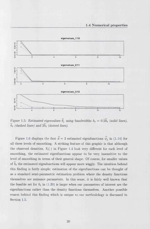
It is clear from Figure 1.5 that for all levels of smoothing, the first two eigen values are much larger than the remaining ones. Indeed, from the third eigenvalue onwards it appears that there is no clear cut-off. This would lead one to conclude that for all levels of smoothing, we have two factors driving the dynamic behavior in the density functions. These findings are supported by Table 1.2 which con tains the P-values from 100 replications of the bootstrap test in Section 1.2.2.3. For all levels of smoothing, we reject the null H0 : 02 = 0 but cannot reject the hypothesis that dj — 0 for j = 3,4,5. We can of course continue to test dj = 0
for j > 6 but there is little point in doing so since if dj = 0 this automatically
[image:29.598.30.521.28.795.2]1.4 N u m e ric a l p ro p e rtie s
eigenvalues_1:10
lr>
+ 0
o co o o
+
0 o
eigenvalues_2:11
eigenvalues_3:12
Figure 1.5: Estimated eigenvalues 6j using bandwidths ht = 0.5ht (solid lines),
ht (dashed lines) and 2ht (dotted lines).
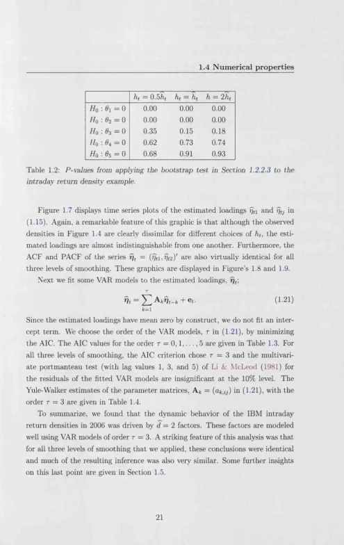
[image:30.597.29.525.36.795.2]ht = 0.5 ht 5- II >9 h = 2ht
Ho : 0i = 0 0.00 0.00 0.00
Ho : #2 = 0 0.00 0.00 0.00
Ho : 03 = 0 0.35 0.15 0.18
Ho : 04 = 0 0.62 0.73 0.74
Ho : 05 = 0 0.68 0.91 0.93
Table 1.2: P-values from applying the bootstrap test in Section 1.2.2.3 to the intraday return density example.
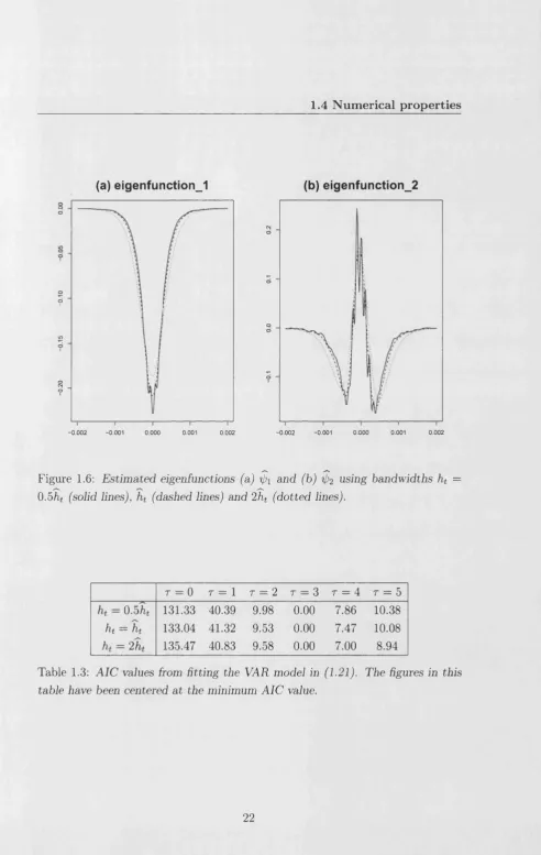
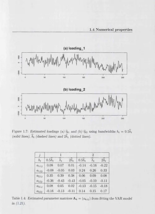
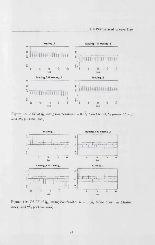
Figure 1.7 displays time series plots of the estimated loadings fjt\ and fjtj in (1.15). Again, a remarkable feature of this graphic is that although the observed densities in Figure 1.4 are clearly dissimilar for different choices of ht, the esti mated loadings are almost indistinguishable from one another. Furthermore, the ACF and PACF of the series fjt = are also virtually identical for all three levels of smoothing. These graphics are displayed in Figure’s 1.8 and 1.9.
Next we fit some VAR models to the estimated loadings, rjt;
T
V t = + e* (L21)
k=i
Since the estimated loadings have mean zero by construct, we do not fit an inter cept term. We choose the order of the VAR models, r in (1.21), by minimizing the AIC. The AIC values for the order r = 0 ,1, . . . , 5 are given in Table 1.3. For all three levels of smoothing, the AIC criterion chose r = 3 and the multivari ate portmanteau test (with lag values 1, 3, and 5) of Li & McLeod (1981) for the residuals of the fitted VAR models are insignificant at the 10% level. The Yule-Walker estimates of the parameter matrices, A*, = (u^ij) in (1.21), with the order r = 3 are given in Table 1.4.
[image:31.595.24.520.25.810.2]1.4 N u m e ric a l p ro p e rtie s
(a) eigenfunction_1 (b) eigenfunction_2
CNJ o
o
o o
?
-0.002 -0.001 0.000 0.001 0.002
§ o
?
o 01
in ?
s ?
-0.002 -0.001 0.000 0.001 0.002
Figure 1.6: Estimated eigenfunctions (a) ipi and (b) using bandwidths ht =
0.5ht (solid lines), ht (dashed lines) and 2ht (dotted lines).
r = 0 r = 1 T = 2 T = 3 T = 4 r = 5
II O Ui >*) 131.33 40.39 9.98 0.00 7.86 10.38
ht — ht 133.04 41.32 9.53 0.00 7.47 10.08
II to >-> 135.47 40.83 9.58 0.00 7.00 8.94
[image:32.595.27.520.27.805.2](a) loading_1
0 50 100 150 200 250
(b) loading_2
CN
O
0 50 100 150 200 250
Figure 1.7: Estimated loadings (a) rjt\ and (b) fft2 using bandwidths ht = 0.5ht (solid lines), ht (dashed lines) and 2ht (dotted lines).
j 1 2
ht 0.5/if ht to
1 >
*) 0 .5 ^
ht 2 ht
Ul,lj 0.08 0.07 0.01 -0.14 -0.16 -0.22
al,2j -0.08 -0.05 0.03 0.24 0.26 0.33
a2,lj 0.35 0.39 0.38 0.06 0.09 0.08
a2,2j -0.36 -0.43 -0.43 -0.05 -0.10 -0.11
a3,lj 0.08 0.05 0.02 -0.13 -0.15 -0.18
f l 3,2j -0.16 -0.13 -0.11 0.14 0.15 0.17
[image:33.598.27.528.25.716.2]1.4 N u m e ric a l p ro p e rtie s
loading_1 loading_1 & loading_2
Mi-t -t - t i l '
tI 'IH:
loading_2 & loading_1 loading_2
Figure 1.8: ACF of rjtj using bandwidths h = 0.5ht (solid lines), ht (dashed lines)
and 2ht (dotted lines).
loading_1 loading_1 & loading_2
10
Lag
15 20 10
Lag
15
loading_2 & l o a d in g ! loading_2
20
. . ( . . . . I ...i. d "
o
o 1 , L . .. i p - L l ,
'• L “ i
i: i 1 f [ |: [ | : ' r f
0 -1
[image:34.597.28.528.24.816.2]...V ...
...f ' T
-2 0 -1 5 -10
Lag
-5 10
Lag
15 20
Figure 1.9: PACF of r)tj using bandwidths h = 0.5ht (solid lines), ht (dashed
1.5
D isc u ssio n
In this chapter, we have developed a method for identifying the finite dimen sionality of curve time series for the realistic setting where the curves of interest are observed with error. Based upon a computational shortcut we have devel oped, the practical implementation of our methodology is trivial even for higher dimensional applications.
We conclude with some remarks which may spur future research. As we saw in the IBM density function example in Section 1.4.2, much of our inference was unaffected by the level of smoothing we applied to the observed densities. In particular, the estimated eigenfunctions had an identical shape for the different bandwidth values we applied.
Consider the standard observational setting
Yij = Xi{Uij) -)- £y, i = 1, . . . , 72, j ' — 1, . . . , 77ij, (1.22)
where Sij is some random noise. Now let Yfy) be a local polynomial estimate of Aj(-). Then in traditional functional data analysis, one is typically interested in estimating the eigenfunctions of A/0(u,u) = Cov{Xj(u), for which we
often use the eigenfunctions of Mo = n _1 Ya=i ( ^ ( u) — — ^"(u)} as our estimates. In this case, it was shown in Hall et al. (2006) that the result ing estimates are root-n consistent, in the £ 2(3) sense, provides m = minm* diverges with n. However, if the observations on each function are sparse, i.e.
m is fixed, and provided that tij are random enough, then the minimax optimal rate of convergence empirical eigenfunctions is n~r^ 2r+1\ Here r is the order of the local polynomial estimator used and thus the number of derivatives assumed on the population functions. The intuition behind this result is simple; under an appropriate set of regularity conditions, if m — > oo, Yfy) is consistent for
Xi(-) and thus M0 is root-n consistent for M0. From here, one can use standard
1.6 P ro o fs
Our setting is different in that we do not require our estimate Yi(•) to be consis tent for Xf(-). In fact to obtain root-n convergence of the eigenfunctions and thus the dynamic space JVC, all we require is that !*(•) has the same auto-correlation structure as Xi(-) or more generally that Mk in (1.9) is root-n consistent for Mk
in (1.3). This leads to an open question;
Given the discrete data design in (1.22), is it possible to construct a
root-n consistent estimate of JVC for the setting where the observations
on each curve Xi(-) are sparse, i.e. m is fixed?
We believe that if this can be achieved, then it would be a significant achievement in the modern era of high dimensional data analysis.
1.6
P ro o fs
In this section we provide the proofs of the propositions in Section 1.2 and the theorems in Section 1.3. Throughout the proofs we may use C to denote a positive and finite constant which may vary from line to line. We refer the reader to Appendix A for some background on operator theory which is required for the proofs. We introduce some technical lemmas first.
Lem m a 1.1 Let L be a finite dimensional operator such that for some sequences
of orthonormal vectors {e^}, {fj}, {gj} and {hj} and some sequences of decreas
ing scalars {dj} and {Aj}, L admits the spectral decompositions L = Y^=i &jej ®
fj = Y lj=i A j gj hj. Then it holds that d! = d.
P ro o f of Lem m a 1.1 Note that if d ^ d' then both Im(L) and Im(L£) will be of different dimensions under the alternative characterizations due to linear independence of {e^}, {fj}, {gj} and {/&j}. Thus it must hold that d = d' . □
P ro o f o f L em m a 1.2 First note that Ker(L*) = (Im(L))x , Ker(L) = (Im(L*))± and Ker(L*) = Ker{LL*). Thus
Im(LL*) = (Im (LL*))X\
= (Im((Lr)*))xx
= (K er(Li*))x
= (Ker(L*))x
= (Im(L))xx
= Im(L),
which concludes the proof. □
For the sake of the simplicity in presentation of the remaining proofs, we adopt the standard notation for operators acting on Hilbert spaces. For any / G £ 2 p ) , we write ||/|| = y/ (/, / ) (see (1.5)), and denote M k f G .C2P ) the image of / under the operator Mk in the sense that
(Mkf)(u ) =
J
Mk(u ,v)f(v)dv.The operators ATfc, K, Mk and K may be expressed in the same manner. Note now that the adjoint operator of Mk is
Furthermore Nk = MkM% in the sense that N k f = M kM ^f; see (1.10). In the
same way K = J2k=i and K = 1 see (1-12) and (1.13).
P ro o f o f P ro p o sitio n 1.1 (i) We only need to show Im(iVfc) = M. Since
Nk = MfcM£, it follows by Lemma 1.2 that Im (Nk) = Im(MkM^) = Im(M^) since both Nk and Mk are finite dimensional and thus their images are closed.
Now, recall from Section 1.2.1 that Mk may be decomposed as
d
M k = Y l ® Vi- (L23)
1.6 Proofs
Thus from (1.23), we may write
= (1-24)
where
Pik
2—1
(fc) ct
- ^ h e ^ h.
5 ^ i < V J t=t
From (1.23), it is clear th at Im (Mk) C M, which is finite dimensional. Thus M k
is compact and therefore admits a spectral decomposition of the form
Mk = i ^ e f )i>f) ®<t>f\ (1.25)
3= 1
with (<jfp, ) forming an adjoint pair of singular functions of Mk corresponding to the singular value 9jk\ Clearly dk < d. Thus if dk < d, lm(Mk) C 3VC since from (1.25), Im(Mfc) = span{V>jfc^ : j = 1 , . . . , d k} and any subset of dk(< d)
linearly independent elements in a d-dimensional space can only span a proper subset of the original space.
Now to complete the proof, we only need to show th at the set of { p ^ } in (1.24) is linearly independent for some k. If this can be done then we are in a position to apply Lemma 1.1. Let (3 be an arbitrary vector in Md and put
cp = (<pi,. . . , ifd)' and p k = (Pifc\ • • •, Pd^y» then the linear independence of the set { p ^ } can easily be seen as the equation
Ppk = P'ZkV = 0,
has a nontrivial solution if and only if /3S*, = 0. However since E*, is of full rank by assumption, it follows that it is invertible and the only solution is the trivial
one (3 = 0. Thus Lemma 1.1 implies dk = d and the result follows from noting
that any linearly independent set of d elements in a d-dimensional vector space forms a basis for that space.
K = Ylk=i Nk is also non-negative definite. Therefore, Im(iir) = U^=1Im(ATfc). Prom here, the result given in part (i) of the proposition concludes the proof. □
P ro o f o f P ro p o sitio n 1.2 Let Qj be a non-zero eigenvalue of K*, and 7 - =
( 7 1 j , • • • , 7n-pj)' be the corresponding eigenvector, i.e. K*7j = Writing
this equation component by component, we obtain that
{Yt+k - Y , Ys+k - Y )(Y , - Y , Y i - Y ) yij = 7^ , (1.26)
^ Pl i,,=i k=i
for t = 1 , . . . , n — p; see (1.16). For ipj defined in (1.17),
(£&)(») =
J
K(u,v)ipj(v)dv= 2 “ ? (U) } ( Y* ~ Y & H Y t + k ~ Y , Ys+k ~ Y )
^ t,s= l fc=l
n—p p
(n — p)2 '
V t,a,i=1 fc=l
5 3 £ { y t(u) - y(u)b«<n ~ y ,y, ~ ? ){Y t+k - ? , Ys+k - y>,
see (1.13). Plugging (1.26) into the right hand side of the above expression, we obtain that
n—p
t=1
i.e. ipj is an eigenfunction of K corresponding to the eigenvalue dj. □
Before presenting the proof of Theorem 1.1, we present a further technical results which proves useful in the derivations.
Lemma 1.3 Let A ,B £ §. Then it holds that \\AA* — BB*\\jj < {||^4||s +
||B ||g }||4 -B ||g .
P ro o f o f Lemma 1.3 First note that for any 4 , B € S, ||^4*||§ = ll^lls and by
the Cauchy-Schwarz inequality ||4B||>r < ||4||g||B||g. Thus
||4 4 * -B B * ||* = ||( 4 - B ) 4 * + B ( 4 * - B ‘)||N
< ||(4 — B)j4*||ff+ || B(j4* — B*)||k
< ||4*||s ||4 - B ||s + ||B ||g ||4 * - B * ||s
1.6 Proofs
as required. □
P ro o f o f T h e o re m 1.1 First notice that
v
II*-*11*
= \\J2Nk-Nk\\n
k= l p
< - MkM'k U
fc=1
p
k=l
where the final inequality follows from Lemma 1.3. Now if Mk Mk in the topology of S, then ||Mjb||g ||Mfc||§ < oo since the existence of E(Yt2) guaran tees that Mk is Hilbert-Schmidt. Thus we may write
p
| | £ - t f | U < A £ | | M * - M t ||*, (1.27)
fc=l
where A = maxfc>i{||A/fc||s + ||Mfc||§}. From (1.27) it is clear that we are only required to control ||Mk — Mk\\s since if this quantity converges to zero, then A will be bounded in probability and K will be consistent in the || • ||n sense.
Now, some straightforward calculations show that
n —p
Mk = - A - Y l ( Y t - ? ) ® ( Y t+k- Y )
n - V T lt= l
n —p
= — y '( V 1 - ^ ) ® ( y m - ^ ) + Op(n -1), (1.28)
n ~ P t (
since n ~ n — p (as p is fixed and finite). P ut Ztk = (Yt ~ f1) ® (Yt+k ~ v) ~ Mk.
as Ztk £ 2loo (which, by conditions C l and C2, guarantees integrability of o;~1(u)Q |Ztfclls (u)). Thus via an application of the Chebyshev inequality to (1.29) it follows that
n —p
Mk - M k = ( n - p ) - 1 Ztk + Op(n~l ) = O ^ tT 1/2). (1.30)
t= 1
Now (1.27) and (1.30) together yield \\K — i f ||n = Op(n~1//2). This concludes the first part of the assertion.
Given \\K — i f ||>f = Op(n ~ ^2), Lemma B.l implies that supJ>:l \6j — 6j\ =
Op(n-1/2). Finally, condition C4 implies that tjjj is an identifiable statistical parameter from which Lemma B.2 in yields \\ipj — i p j || = Op(n_ly/2) for j = 1 ,. . . , d since we always assume that the right versions (in terms of sign) of i p j and i p j are
used. □
Lem m a 1.4 The function D defined in (1.18) is a well defined distance measure
on Z.
P roof o f Lemma 1.4 Non-negativity, symmetry and the identity of indis-
cernibles are obvious. It only remains to prove the subadditivity property. For any L G §, note th at ||L||g = y/tr(L*L), where tr denotes the trace operator. Now, for any X* E Z, i = 1, 2,3, let II Xj denote its corresponding d dimensional projection operators defined as follows
d
n x , = ^ ^ Ci j ® Cij j
3= 1
where {£y : j = 1, . . . , d} is some orthonormal basis of X*.
Now the triangle inequality for the Hilbert-Schmidt norm yields
l|nXl - fix3 ||s < ||nXl - nx2||s + ||nx2 -
nx3||s-Since the projection operators are self adjoint, we have
\A r ( n ^ ) + t r ( n ^ ) - 2 tr(n XlIIx3)
1.6 Proofs
Now tr(II^ ) = trQnxJ = d and t r ^ I I x , ) = Tfi,k=1 (CihCjkf for i , j = 1,2,3. These last facts along with the definition of D in (1.18) give
D{X1:X3) < D(X1,X2) + D(X2,X 3),
which concludes the proof. □
P ro o f o f T h e o re m 1.2 (i) First note that from (1.18)
V M D (M I3VC) =
||n3;t - n M||s>
(1.31)
where ILj^ = 52j=1 ipj <8>ipj and IIm = <pj ® 4>j with 0 i , . . . , fa forming any orthonormal basis of M. Now if 11^ and 11^ are any projection operators onto M, then by virtue of Lemma 1.4 it holds th at HII^ — II^Hs = y/2D(M, M) = 0. Thus we may proceed as if Iljvt in (1.31) was formed with eigenfunctions of K , i.e. <j)j = ipj for j = 1, . . . , d.
Now we have
d d d
I I ® ^ l | s < (1*32)
j=i j=i j=i
i.e. ipj <8>ipj (resp. ipj <g> ipj) is the projection operator onto the eigensubspace generated by 6j (resp. 6 j) . Now by Theorem 1.1, | | K —K \ \jj > \ \ K — K \\§ =
Op(n-1/2). Thus an application of Lemma B.4 yields \\ipj ® ipj — ipj ® ipj\\% —
Op(n~1/2) for j = 1 , . . . , d . This last fact along with (1.31) and (1.32) yield
D (M ,M ) = Op(n-1/2).
(ii) It remains to prove the adaptivity property. For any constant C > 0
P {n 1/2\D '(U ,M ) - D (M ,M )| > C}
= P { n 1/2\D '{M ,M ) - DpVt,M)| > C, d = d}
+ P {n l/2\D '(M ,M ) - D(jfC,M), d ^ d}
= P {n 1/2\ D \ M , M ) - D ( M :M ) \ > C \ d = d}P(d = d)
+ P {n 1/2\D '(M ,M ) - P(M,3VC)| > C \ d ^ d}P(d ^ d)
< P {n 1/2\D '(M ,M ) - D (M ,U )\ > C \ d = d}P(d = d) + P(d ± d)(1.33)
Now by assumption P(d = d) — > 1 and thus P{d ^ d) = o(l). Furthermore, if
M eth o d o lo g y a n d convergence
ra te s for fa c to r m o d elin g of
m u ltip le tim e series
2.1
In tr o d u c tio n
When modelling a time series Y t G Mp, a crucial task in any pre-analysis is to try and reduce the dimensionality if p is large. To see why, if one tries to fit a VAR model to Y t then we are required to estimate 0{p2) parameters and in many modern statistical data sets we may have p « n or even p » n, where n
is the sample size. In these settings, our estimation is likely to be inaccurate and we may end up making misleading inferences as a result. This is the so called “curse of dimensionality” and is at the forefront of modern statistical research; see Donoho (2000) and Fan & Li (2006).
There have been many attempts in reducing the dimensionality for multiple time series which include principal component based approaches (Preistley et al.
(1974) and Stock & Watson (2002)), canonical correlation based methods (Box & Tiao (1977) and Tiao & Tsay (1989)) and factor models (Bai (2003), Engle k
Watson (1981), Forni et al. (2000), Lam k Yao (2009), Pena & Box (1987) and Pan k Yao (2008)).
2.1 In tr o d u c tio n
Pan & Yao (2008) who identified the factor loading space by expanding the white noise space step by step and used portmanteau tests as a stopping rule. Although our estimation procedure is based upon the same principle as Pan & Yao (2008), our implementation is much more efficient and can handle cases with very large
p. See also Lam & Yao (2009). An interesting feature of our methodology is that nonstationarity is permitted and does not necessarily have to be driven by unit roots. The latter was consider in Ahn (1997) and Pena & Poncela (2006). In fact, all that is required to obtain consistency of the factor loading space is that the sample autocovariance matrices are consistent for their population counterparts. This is often implied by ergodicity of a stationary process and may also be fulfilled by some non-stationary mixing processes; see the remarks made in Section 2.3.
The main focus of this chapter is on identifying the number of latent factors. To this end, we present a simple white noise test and provide some theory to support it. In particular, we argue that the number of factors is equal to the number of non-zero eigenvalues of a p x p matrix, which is simply a function of the population autocovariance matrices. Although the sample analogue of this matrix is likely to be full ranked, we prove a striking result which is unique to our methodology; the eigenvalues whose population counterparts are truly zero are “super-consistent” under an ideal set of condition, i.e. they converge to zero at the rate n -1. An example of a consistent threshold based estimator of the number of latent factors is also given.
2.2
M eth od ology
2.2.1 F actor m od els
Let
Y t
be a p x 1 time series generated by the factor modelY t = A X t + £i, t = l , . . . , n , (2-1)
where X* is a d x 1 time series with d < punknown, A is a px d unknown constant matrix and et is a p x 1 white noise process in the sense that E ( e se ,t) = 0 for
any s ^ t. Note that we do not lose any generality by assuming that et is a
white noise sequence since if this was not the case then any parts of et which possess serial correlation should be absorbed into X*. Conversely, we may also assume that there exists no linear combination of X* which is a white noise process otherwise such a linear combination may be absorbed into et. We only observe Y i , . . . , Y n from the factor model (2.1). To simplify the presentation, we assume that E {
Y t)
= 0. In practice this amounts to replacing Y* by
Y t
— Y before the analysis, where Y = n~l Ylt=iYt-The components of X t are called the common factors and A is called the factor loading matrix. We may assume that the rank of A is d since if this is not the case then (2.1) may be expressed equivalently using a smaller number of factors. Note that model (2.1) is unchanged if we replace A and X* by A H and H - 1X* for any invertible d x d matrix H. Therefore, we may assume that the columns vectors of A = ( a i , . . . , a^) are orthonormal, i.e.
A 'A = Id, (2.2)
where Id denotes that d x d identity matrix. Note that even with the constraint in (2.2), A and X* are still not uniquely determined in (2.1) as the aforementioned replacement is still applicable for any invertible H. However, the linear space spanned by the columns of A, denoted M and called the factor loading space, is a uniquely defined d-dimensional subspace of Rp; see the arguments in Section
2.2 M ethodology
2.2.2
E stim a tio n o f JVC
Let £„(*) = E ( Y tY't+k) and Hx(k) = £ (X tXJ+fc) denote the lag autocovari ance matrices of
Y t
and X t respectively. We impose the following identifiability conditions:Al. £s is a white noise sequence uncorrelated with X* for all s, t.
A2. rank{Ex(A;)} = d for some 1 < k < q.
Then under conditions A l and A2, Proposition 1.1 in Chapter 1 implies that the matrix L q defined by
L , = £ £ „ ( * ) £ # ) ' , q > 1, (2.3)
k= 1
has exactly d non-zero eigenvalues and M is the linear space spanned by the corresponding eigenvectors.
A formal proof of this result is given in Chapter 1 in the more general setting where the observations are functional. However, in the vector case it is much easier to see the reasoning behind this result. Under the assumption that X s and
et are uncorrelated for all s, t it follows that
£„(*)£»(*)' = A £ x(fc)£x(/c)'A', (2.4)
since A 'A = 1^; see (2.2). Thus from (2.4) it is clear th at the eigenvectors of S y(A;)Sy(k)' are elements of M. In addition, it is clear th at rank{Sy(/[;)Ey(/c)/} < d with equality if and only if rank{Sa;(A:)} = d. Thus if rank{Xx(A;)} = d,
it holds that Ey(fc)Sy(/c)/ has exactly d uniquely determined eigenvectors (up to sign provided th at the eigenvalues are all different) corresponding to d non-zero eigenvalues. By noting these last few facts, the result above follows by recalling that d linearly independent vectors in a d-dimensional space form a basis for that space.
S y(A:)Sj/(A:)/ may be replaced by 'Zy(k) in all of the discussion in the preceding paragraph. However it does not necessarily hold that Y ll=1 has exactly d
non-zero eigenvalues due to the fact that the matrices E y(A;) are not non-negative definite.
R em ark 2.1 (i) A l is relaxed in Pan & Yao (2008) to allow for correlations between X s and et. Their methodology relies on estimating M -1 = spanje^ G Mp : e' fj = 0 Vfj G M} via a stepwise expansion algorithm. However, the minimization problem implicit to their algorithm is p dimensional at each step. Thus if p is large the methodology developed there may not be computationally feasible.
(ii) The condition that rank{£x(/c)} = d for some k > 1 holds without loss of generality since if this was not the the case then the parts of X* without any serial correlation should be confounded into et.
In light of the arguments above, we may estimate JVt as follows. Let £ y(fc) = (n — k ) - 1 Ylt=i then we define our estimator of Lg by
L, = ^ S „ ( f c ) S y(fc)'. (2.5)
k=1
Now our estimator of d is the number of “non-zero” eigenvalues of Lq (see Section 2.2.3 below) and our estimator of M is the linear space spanned by the corre sponding eigenvectors. Note that both L9 in (2.3) and Lq in (2.5) are non-negative definite, thus all of their eigenvalues will be greater than or equal to zero.
2.2.3
W h ite noise te st for
dLet Ai > • • • > Xp > 0 denote the ordered eigenvalues of L q in (2.3) and recall that under identifiability conditions Al and A2, it holds that rank{Lg} = d,
2.2 M ethodology
Aj > e}. Provided e tends to zero at ah appropriate rate, Theorem 2.3 shows
th at such a method for estimating d is consistent. Further theoretical evidence in favor of this method is supported by the striking result in Theorem 2.2 which suggests that the convergence rates of the eigenvalues Aj for j > d + 1 is n -1 when an ideal set of conditions are satisfied; i.e. the estimated eigenvalues whose population counterparts are truly zero are “super-consistent” . Some intuition behind this result is given in Section 2.3 and simulation evidence is provided in Section 2.4.
A more useful data driven method of estimating d is given by the following “white noise test” . Suppose that we are interested in testing the hypothesis
Ho : d = do, 1 < do < p. (2.6)
Then since rank{Lg} = d, testing the hypothesis i