Investigating the Effect of Engine Lubricant Viscosity on Engine Friction and Fuel Economy of a Diesel Engine

University of Huddersfield Repository

Investigating the Effect of Engine Lubricant Viscosity on Engine Friction and Fuel Economy of a  Diesel Engine

Original Citation

Singh, Devendra (2011) Investigating the Effect of Engine Lubricant Viscosity on Engine Friction  and Fuel Economy of a Diesel Engine. Masters thesis, University of Huddersfield. 

This version is available at http://eprints.hud.ac.uk/id/eprint/14060/

The University Repository is a digital collection of the research output of the University, available on Open Access. Copyright and Moral Rights for the items on this site are retained by the individual author and/or other copyright owners. Users may access full items free of charge; copies of full text items generally can be reproduced, displayed or performed and given to third parties in any format or medium for personal research or study, educational or not­for­profit purposes without prior permission or charge, provided:

• The authors, title and full bibliographic details is credited in any copy;

• A hyperlink and/or URL is included for the original metadata page; and

• The content is not changed in any way.

For more information, including our policy and submission procedure, please contact the Repository Team at: E.mailbox@hud.ac.uk.

1 | P a g e

University of Huddersfield, UK

School of Computing and Engineering

(Mechanical Engineering)

Investigating the Effect of Engine Lubricant Viscosity on

Engine Friction and Fuel Economy of a Diesel Engine

Submitted by

Devendra Singh

Supervisor:

Prof. John D. Fieldhouse

(Automotive Research Group, SCE, UoH, UK)

Co-Supervisors:

Prof. D.R.Brown

(Department of Chemical and Biological Sciences, UoH, UK)

Sh. A.K.Jain

(Scientist G, Indian Institute of Petroleum, CSIR, Dehradun)

A Dissertation Submitted to SCE in Partial fulfillment of the requirements for the

Degree of Master of Science by Research in Mechanical Engineering

2 | P a g e ACKNOWLEDGEMNT

The author would like to express his gratitude to Prof. John.D.Fieldhouse, Automotive Engineering Group, School of Computing and Engineering, and Prof D.Rob.Brown, University of Huddersfield, UK for their keen interest, inspiring guidance, helpful suggestion and providing the quintessential environment to conduct this research work. Special mention has to be made of Dr. Fengshou Gu, for all of the technical insight and help provided in analysing the data on numerous occasions during the project work.

The author would also like to thank British Council, UK and DST, India for approving a joint project UKIERI Research award, under which author got an opportunity to undertake this small piece of work. Author is indebted to Dr. M.O.Garg, Director IIP, Dehradun for being the main

source of inspiration behind this research work.

My sincere thanks are due to Dr M.R.Tyagi, Head Tribology Division, Dr S.K.Singal, Head Automotive Fuels and Lubes Application Division, Sh A.K.Jain, Scientist G, Sh Nishan Singh, Scientist G and other colleagues of Indian Institute of Petroleum, Dehradun, for their valuable suggestion and continuous encouragement in carrying out this work.

Last but not the least thanks are due to all the team members of the UKIERI Joint project between IIP-CSIR, India and UoH, UK for their kind support and help provided during the project work. Finally, I would like to thank my parents; my wife and other family members for all support provided during the project work and would like to dedicate this dissertation to my son Divyanshu for giving me a very important reason to remain happy.

3 | P a g e COPYRIGHT STATEMENT

i. The author of this thesis (including any appendices and/or schedules to this thesis) owns any copyright in it (the “Copyright”) and he has given The University of Huddersfield the right to use such Copyright for any administrative, promotional, educational and/or teaching purposes.

ii. Copies of this thesis, either in full or in extracts, may be made only in accordance with the regulations of the University Library. Details of these regulations may be obtained from the Librarian. This page must form part of any such copies made.

iii. The ownership of any patents, designs, trademarks and any and all other intellectual property rights except for the Copyright (the “Intellectual Property Rights”) and any reproductions of copyright works, for example graphs and tables (“Reproductions”), which may be described in this thesis, may not be owned by the author and may be

4 | P a g e ABSTRACT

Fuel economy is affected, both by fuel and engine lubricant quality. Engine lubricant quality plays a vital role in reduction of fuel consumption by effective reduction of friction between the contact surfaces of engine parts (piston ring assembly, bearings and valve train). Engine components are exposed to various lubrication regimes such as hydrodynamic, elasto-hydrodynamic, boundary and mixed lubrication during engine operation. In each of these regimes, the factors which influence engine friction are different. Hydrodynamic friction is influenced by lubricant rheology, film thickness and sliding speed of interacting surfaces, whereas boundary and elasto-hydrodynamic friction is a function of surface properties like roughness and hardness and the type of friction modifier used in engine lubricant. So the

principal factors which influence engine friction power are speed, load, and surface topography of engine components, oil viscosity, oil temperature and type of friction modifiers used.

It is generally accepted that both the piston assembly and bearings are predominantly in the hydrodynamic lubrication regime, whereas the valve train is in the mixed/boundary lubrication regime. Hydrodynamic friction is proportional to sliding velocity of a pair, oil film thickness, operating temperature, lubricant viscosity and many other physical parameters.

5 | P a g e

consumption and Fuel Efficiency (%FE) for the light duty IDI diesel engine were analyzed for both engine lubricants.

In order to determine the most dominant factor among the engine operating conditions such as speed, load and engine lubricant viscosity, which affect engine friction power significantly, a full factorial design of experiments (DOE) was formulated to analyze some of the important parameters by which engine friction power influenced significantly. Three factors; speed, load and oil viscosity were chosen as variables with each factor having two levels.

Statistical analysis for determining the dominant factor, affecting the friction power of an engine revealed that the engine speed and speed-load combination are the most significant factors on which engine friction is strongly influenced. An empirical model was developed based

6 | P a g e TABLE OF CONTENT

Abstract 4

Overview of the Thesis 11

1. Introduction and Objectives 13

2. Literature Review 19

3. Engine Friction Basics 22

3.1 Piston ring liner friction 25

3.2 Bearing friction governing equation 28

4. Engine Friction Measurement Technique 31

5. Experimental Details for DI Heavy Duty Diesel Engine 33

5.1 Results and Discussion for DI Engine 36

6. Experimental Details for IDI Light Duty Diesel Engine 45

6.1 Results and Discussion for IDI Engine 47

7. Analysis of Dominant Factor Influencing Friction Power by DOE 50

8. Conclusion and Recommendation 57

9. References 59

10. Annexure I 61

Matlab Programme for cylinder pressure

11. Annexure II 65

Factorial Fit: FP (kW) versus speed, load and viscosity

All factors with main effects, first order interaction and second order interaction

12. Annexure III 66

Factorial Fit: FP (kW) versus speed, load and viscosity

7 | P a g e List of Tables

Table 1. Fully warmed up engine friction power losses in W 20

Table 2. Engine specifications for DI 33

Table 3. Test operating conditions 34

Table 4. Physical characteristics of both engine lubricants 35

Table 5. Pressure sensor specifications 35

Table 6. Mean effective Pressures at different load for engine lubricant 37 SAE 20W-50 at both speeds

Table 7. Mean effective Pressures at different load for engine lubricant 38 SAE 10W-30 at both speeds

Table 8. Indicated power (IP), Brake power (BP) and Friction power (FP) 40 for both oils under prescribed engine operating conditions

Table 9. Percentage reduction of bsfc (g/kWh) of an engine operating 44

at 2000 rpm

Table 10. Test engine specification for IDI 45

Table 11. Induction Run Test cycle 47

Table 12. Test results of full load Performance of engine charged 47

with Engine Oil ‘C’

Table 13. Test results of full load Performance of engine charged 48

with Engine Oil ‘D’

Table 14. Comparative results of bsfc (g/kWh) for both engine lubricants 48 at different speeds under steady state conditions

Table 15. Factors with its levels of experiment 50

Table 16. Physical characteristics of both engine lubricants 50

Table 17. Full Factorial Design of Experiment with Response Variable 52

Friction Power (FP), kW

8 | P a g e List of Figures

Fig 1. Energy Distribution 14

Fig 2. Global production of different types of vehicles 14

Fig 3. Four valves per cylinder 15

Fig 4. V-type Internal Combustion Engine 16

Fig 5. Stribeck curve representing different lubrication regime 17

Fig 6. Distribution of the total mechanical losses of a diesel engine 19 Fig 7. Stribeck Diagram for journal bearing; Coefficient of friction, f 22 versus dimensionless duty parameter, µN/σ

Fig 8. Schematic of two surfaces in relative motion under boundary 23

lubrication conditions

Fig 9. Schematic of hydrodynamic oil film between liner and piston, 26 assuming liner is moving

Fig 10. Critical parts of engine 28

Fig 11. Film geometry of the typical journal bearings 29

Fig 12. Test bench setup 34

Fig 13. Schematic representation of experimental test set-up 34

Fig 14. Graphical representation of variation of mean effective pressures 38 with load for engine lubricant SAE 20W50 at both speed

Fig 15. Graphical representation of variation of mean effective pressures 39 with load for engine lubricant SAE 10W-30 at both speed

Fig 16. Comparison of Friction mean effective pressure, FMEP vs torque 40 for both engine lubricants

Fig 17. Engine friction power at different operating conditions for both oils 41 Fig 18. Comparative Performance characteristics curves for both engine oils 49

Fig 19. Comparative bsfc (g/kWh) of Oil C and Oil D 49

Fig 20. Normal plot of all factors (effects) influencing 54

the response Friction Power

Fig 21. Pareto Chart for all factors (effects) influencing 54

9 | P a g e

Fig 22. Main Factors (effects) plot speed, load and lubricant viscosity for 55 the response Friction Power

Fig 23. Interaction Plot of speed-load, speed-viscosity, load-viscosity 55 for the response Friction Power

NOMENCLATURE Symbol Description

B Width of the ring

C Bearing clearance (R1-R2)

∂P/∂x Pressure gradient along the width of piston ring

∂P/∂y Pressure gradient in circumferential direction of a piston ring ∂P/∂z Pressure gradient through film thickness

dh/dx Film thickness gradient along the ring width

Fn Normal load

Ft Force required for tangential motion

f Coefficient of friction

fs Metal–to-metal coefficient of dry friction

fL Hydrodynamic coefficient of friction

h Film thickness

h1 Film thickness at the entrance

h2 Film thickness at the start of cavitation region

hmin Film thickness corresponding to the maximum pressure M1, M2 Fuel consumptions at steady state

N rotational speed of the shaft (rpm)

P1 and P2 Pressure at entrance and exit of ring face

qx Flow rate per unit circumferential length of a ring

R1 andR2 Radius of bush and shaft

U Velocity of liner

V Velocity of a ring in circumferential direction

wh, wo Velocity of top and bottom layer

10 | P a g e

µ,η Dynamic viscosity of the lubricant

σ loading force per unit area

σm yield stress of the material

Vd Displacement volume

ω angular speed (rad/s)

ABBREVIATIONS

BDC Bottom Dead Center of an engine cylinder

BMEP Brake Mean Effective Pressure

BP Brake Power

bsfc Brake Specific fuel consumption

CI Compression Ignition

DOE Design of Experiment

DI Direct Injection engine

FE Fuel efficiency

FMEP Friction Mean Effective Pressure

FP Friction Power

IP Indicated Power

IDI Indirect Injection engine

IMEP Indicated Mean Effective Pressure

rpm revolutions per minute

11 | P a g e OVERVIEW OF THE THESIS

This thesis has been written with a perspective to investigate the effect of engine lubricant viscosity on engine friction and fuel consumption of a diesel engine. The engine components

resulting in the majority of engine friction are; piston ring assembly, valve train system, bearing system and engine powered auxiliaries (such as the water pump, oil pump, fuel pump etc.). Piston ring assembly and bearings are predominantly operating in the hydrodynamic lubrication regime and contribute significantly towards engine friction losses, whereas the valve train system operates in the mixed/boundary lubrication regime, also plays vital role towards engine friction. Hydrodynamic friction is influenced by lubricant viscosity, sliding velocity and oil film thickness whereas boundary/mixed friction is dependent on the surface properties such as roughness, hardness, elasticity, plasticity, shearing strength, of sliding pair factor as well as by lubricant properties like friction modifiers.

The main focus of this thesis is to understand and investigate the effect of engine lubricant viscosity on engine friction and fuel consumption of a diesel engine, theoretically and experimentally. It has also been attempted to determine the most dominating factor among engine operating condition; speed, load and viscosity, which affect engine friction significantly. This thesis is arranged in four major sections. The first section (Chapter 1 to 3) provides an introduction, aims or objectives and literature review related to scope of research work, where the need of this study is highlighted and clearly defines the objectives of the proposed research work undertaken.

The second section (4 and 5) focuses on the basics of friction using a stribeck curve to describe the different lubrication regimes such as boundary, mixed and hydrodynamic. Further, hydrodynamic friction for engine bearings and piston ring assembly is being derived

theoretically using Reynolds equations. This section also highlights some of the standard measurement technique known, for engine friction measurements.

12 | P a g e

IMEP which in-turn is used for calculating FMEP and friction power of an engine. Test results in terms of Friction mean effective pressure, friction power and brake specific fuel consumption are also discussed for different viscosity grade engine lubricants.

Fourth and the last section (8 and 9) of this thesis focuses on the identification of the dominant factor among; engine operating conditions (speed and load) and viscosity of lubricant, which influences friction power significantly using a full factorial method of Design of experiment approach. In this section empirical relation is also developed for analyzing the significant factor affecting engine friction. This section also provides some concluding remarks and recommendation for future studies. Chapter 10 is the reference /Bibliography section which describes the research paper referred while writing this thesis. Finally Annexure I provide the

13 | P a g e Chapter 1

INTRODUCTION AND OBJECTIVES

Economy, Efficiency, Effectiveness and Ecology form the four significant pillars for sustainable growth of any nation. Worldwide, crude oil prices were very unstable during 2008-09, peaking up to $145 per barrel in July 2008 before coming down at the end of year 2009, but again the price is reaching to $100 per barrel during year 2010-2011. Hence crude oil price has become a matter of great concern for everyone.

Combined with the demands of crude oil the drive towards low carbon emissions, and the recognition that current fossil fuel supplies are predicted to last possibly only 40 years, has focused the attention of the automotive industry to towards alternative fuels supplies and

improved engine efficiency.

Figure 1 shows the general energy distribution of energy where it is seen that road transportation demands almost 16% of the available fuel sources. This is distributed between commercial vehicles and domestic vehicles as indicated in figure 2. It can be seen that in general terms the industry is producing some 90 million units per year into a global market that already supports some one billion (109) units. Based on fundamental and conservative figures of 10,000

miles/year per unit this gives 10 × 1012 miles per year. If a consumption of 7 miles/litre is

assumed then this represents a fuel demand of 1.4 × 1012 litres per year. Clearly with such demands, which continues to increase, then there is a need to seek a means to reduce fuel consumption by improved engine efficiencies - and improved lubrication is one way forward.

World lubricant demand will increase 1.6 percent per year to 40.5 million metric tons in 2012 [1] and India is the third largest consumer of lubricants in Asia, India’s overall lubricants

market is expected to grow 3.7 percent per year to reach 2.2 million metric tons by 2014 [2]. India spends substantial amount of nation’s revenue in importing approximately 70% of total

14 | P a g e

Figure 1. Energy Distribution

Figure 2. Global production of different types of vehicles

15 | P a g e

It is now of major concern that exhaust emissions are seen as a global threat so improving the efficiency of the power-train is a priority. Regulations of exhaust emissions and fuel economy are the main driving force behind the development of advanced IC engines. Automotive industries are putting significant amount of efforts in designing the fuel efficient vehicle by adopting latest engine technology in order to conserve the fuel.

Figure 3. Four valves per cylinder

On the engineering side, manufacturers of Passenger cars have introduced 4-valves per cylinder (figure 3), roller follower valve train systems, lighter aluminum engines, smaller engine bearings

and gasoline direct injection engines and catalytic converters. Similarly, there have been many advances in the design of heavy duty diesel engines over recent years including the introduction

16 | P a g e

Figure 4. V-type Internal Combustion Engine

Automotive sector consumes a major portion of the petroleum products and in India only its consumption (by automotive sector) is around 60%. Historical studies indicate 10 to 15 % of

17 | P a g e

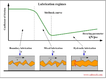
The critical engine components resulting in the majority of engine friction are; piston ring/liner

assembly, bearing system, valve train system, and engine powered auxiliaries (such as the water pump, oil pump and fuel pump). It is generally accepted that both the piston assembly and bearings are operating predominantly in the hydrodynamic lubrication regime, whereas the valve train system is operating in the mixed/boundary lubrication regime.

Figure 5. Stribeck curve representing different lubrication regime

The friction due to hydrodynamic lubrication regime (piston ring/liner assembly and bearing

18 | P a g e

both types of lubrication by tailoring the viscosity characteristics of the base oil and the chemistry of the friction-modifying additives.

Aims and Objectives

The focus of this research work is to investigate the effect of engine lubricant viscosity on engine friction characteristics and fuel consumption of a diesel engine theoretically and experimentally. Another important objective is to identify the dominant factor among speed, load and lubricant viscosity, which affect engine friction power significantly through a DOE approach. Engine friction study has been a topic of research for many years. Some of the conventional methods like Morse test, PV diagram, Willans lines method and motoring test for measuring friction of an engine are described in the literature [5]. It is widely accepted that PV diagram method yield

19 | P a g e Chapter 2

LITERATURE REVIEW

The critical engine components resulting in the majority of engine friction are; piston ring/liner

assembly, bearing system, valve train system, and engine powered auxiliaries (such as the water pump, oil pump and fuel pump). To optimize the effects of lubrication many researchers have studied the frictional contribution of individual engine components both theoretically and

experimentally through the use of fired and motored laboratory engine tests. Typical distribution of the mechanical losses in a diesel engine is given in the figure 6. It can be deciphered from the pie chart that piston ring assembly and bearings contributes to approximately 70% of the total

mechanical losses. Two-thirds of the friction losses in an engine are estimated to occur during

the hydrodynamic lubrication of components (piston ring/liner assembly, bearings) and one-third during boundary lubrication or mixed lubrication components.

Figure 6. Distribution of the total mechanical losses of a diesel engine [6, 7].

It is a well accepted fact that the piston ring assembly and engine bearings operate predominantly in the hydrodynamic lubrication regime during engine operation. Hydrodynamic lubrication friction is related to the lubricant viscosity. Effect of engine oil viscosity on engine friction and fuel consumption was studied by many researchers. Radimko Gligorijevic et.al. [8] Describes the effect of lubricants of different viscosity grades on the fully warmed up engine friction power

Engine auxillaries 20% to 25%

Valve Train 7% to 15%

Engine bearings 20% to 30% Piston ring

20 | P a g e

loss (W) - which includes piston ring assembly (P), Valve train (V) and bearing (B). Table 1 shows that total friction power losses are low for the less viscosity grade oil and the power loss through piston ring assembly reduces significantly when lower viscosity grade lubricants was used.

Table 1: Fully warmed up engine friction power losses in W

SAE Grade 10 W 30 15 W 40 20 W 50

Total Losses (W) 1455 1513 1577

P (W) 528 (36%) 639 (42%) 807 (52%)

V (W) 371 (26%) 287 (19%) 140 (9%)

B (W) 555 (38%) 587 (39%) 630 (40%)

Taylor [9] has reported that the friction losses in the piston assembly vary as √ηω, where η is the lubricant dynamic viscosity (mPa.s) (calculated at a temperature representative of the piston assembly) and ω is the angular speed (rad/s) of the engine.

For journal bearings, under light loaded conditions, petroff equation [10] suggested that the friction power loss would vary linearly with lubricant viscosity.

F = 2πηω2LR3 / c

Where F is the friction power loss (watts), η is the lubricant dynamic viscosity (mPa.s) appropriate to the bearing, ω is the engine’s angular speed (rad/s), L is the bearing width (m), R is the bearing radius (m) and c is the bearing radial clearance (m). For a heavily loaded bearing, Taylor [11] has shown that the friction power loss would vary as η0.75. Effects of engine oil viscosity on fuel consumption were studied by Taylor and it has been reported that low viscosity oil results in low fuel consumption [12].

Piston rings act as sealing between the liner and the piston by making thin oil film during their operation. Furuhama [13] incorporated, for the first time the squeeze film effect in the Reynolds

21 | P a g e

18] on predicting piston ring assembly friction loss in firing engine using the indicated mean effective pressure (IMEP) method and validating the model by experimental study is remarkable. Mufti et.al [19] also investigated the influence of engine operating conditions and engine lubricant rheology on the distribution of power loss at engine componentlevel. The study was carried out under realistic fired conditions using a single cylinder gasoline engine. A similar study for assessing the effect of engine lubricant rheology on piston skirt friction was undertaken by A. Kellaci et. al. [20] by developing a piston skirt lubrication model based on a modified Reynolds equation. The results of tribological characteristics such as the movement of the piston, the minimum film thickness, the frictional force and friction power loss were studied in relation to the oil viscosity. It was concluded that oil viscosity directly affects friction in the

hydrodynamic regime. The best design involves obtaining a system that operates principally in a hydrodynamic lubrication regime using low viscosity oil.

22 | P a g e Chapter 3

ENGINE FRICTION BASICS

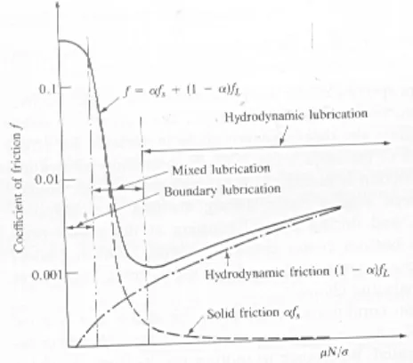
In order to maximize the fuel economy of an engine lubricant one must first understand the source of the friction. Engine friction and friction in general, can roughly be compartmentalized into two groups: coulomb friction (dry friction) which occurs when asperities come into contact between two surfaces moving relative to each other and fluid friction which develops between adjacent layers of fluid moving at different velocities. The actual degree of friction in engine components can seldom be put into either of these categories, and instead lies somewhere between these two extremes. The different regimes of lubricated friction can be illustrated by means of Stribeck curve shown in figure 7, where the coefficient of friction (f) for a journal

bearing is plotted against a dimensionless duty parameter (µN/σ), where µ is the dynamic viscosity of the lubricant, N is the rotational speed of the shaft and σ is the loading force per unit area.

Figure 7. Stribeck curve for journal bearing, Coefficient of friction, f versus dimensionless duty parameter, µN/σ [5]

The coefficient of friction can be expressed as

f = αfs + (1- α) fL where, fs is the metal–to-metal coefficient of dry friction

fL is the hydrodynamic coefficient of friction

23 | P a g e

As α→ 1, f→ fs and the friction is called boundary, i.e closed to solid friction. The lubricating

film is reduced to one or a few molecular layer and cannot prevent metal–to-metal contact between surface asperities.

As α→ 0, f→ fL and the friction is called hydrodynamic or viscous film. The lubricant film

thickness is sufficient to separate the surfaces in relative motion. In between these regimes, there is a mixed or partial lubrication regime where the transition from boundary to hydrodynamic lubrication occurs. While the figure 7 applies to journal bearings, this discussion holds for any pair of engine parts in relative motion with lubricant in between.

Under boundary lubrication conditions, the friction between two surfaces in relative motion is determined by surface properties as well as by lubricant properties. The important surface properties are roughness, hardness, elasticity, plasticity, shearing strength, thermal conductivity and wettability with respect to the lubricant. Figure 8 shows two surfaces under boundary lubrication conditions. Due to the surface asperities, the real contact area is much less than the apparent contact area. The real contact area Ar is equal to the normal load Fn divided by the yield

stress of the material σm;

Ar = Fn/ σm

The force required to cause tangential motion (Ft) is the product of the real contact area and the shear strength of the material τm;

Ft = Ar* τm

24 | P a g e

Thus the coefficient of friction f is

f = (Ft / Fn) = (τm / σm)

For dissimilar materials, the properties of the weaker material dominate the friction behavior. Under boundary lubrication conditions, the coefficient of friction is essentially independent of speed. Boundary lubrication occurs between engine parts during starting and stopping (bearings, piston and rings) and during normal running at piston TDC and BDC, slow moving parts such as valve stems and rocker arms and crankshaft timing gears.

Hydrodynamic lubrication conditions occur when the shape and relative motion of the sliding surfaces form a liquid film in which there is sufficient pressure to keep the surfaces separated. Resistance to motion results from the shear forces within the liquid film and not from the

interaction between surface irregularities, as was the case under boundary lubrication. The shear stress τ in a liquid film between two surfaces in relative motion is given by

τ = µ (dv/dy)

Where, µ is the fluid viscosity and (dv/dy) the velocity gradient across the film. Hence, the friction coefficient (shear stress/normal load stress) in this regime will be proportional to viscosity × speed ÷ loading; i.e., a straight line on the stribeck diagram. Full hydrodynamic lubrication or viscous friction is independent of the material or roughness of the parts and only property of lubricant involved is its viscosity. Hydrodynamic lubrication is present between two converging surfaces, moving at relatively high speed in relation to each other and withstanding a limited loaded, each time an oil film can formed. This type of lubrication is encounter in engine bearings, between piston skirt and cylinder liner and between piston rings and liner for high sliding velocities in mid stroke region.

25 | P a g e 3.1 PISTON RING/LINER FRICTION

It is assumed that compression ring operates in hydrodynamic regime during most of its operating time. Hence the governing equation for piston ring/liner could be Reynolds equation. Now for analyzing the pressure distribution, load capacity, friction force, coefficient of friction etc of piston ring assembly it is necessary to define some important parameters like profile of the ring face, viscosity of oil that keeps piston ring and liner separated during operation, speed of the ring etc. Full Reynolds equation [12] in three dimensional forms for any bearing is given below, here ∂P/∂z = 0, assuming pressure constant throughout the film

∂/∂x(h3_∂

P/∂x) + ∂/∂y(h3∂P/∂y) = 6η (Udh/dx + Vdh/dy) + 12 η (wh-wo) (1)

Simplifying this equation for piston ring, by assuming an infinitely long bearing, very small width as compared to the circumferential length, pressure gradient in circumferential direction can be neglected i.e ∂P/∂y=0. And also velocity in y direction is assumed to be zero i.e V=0 and assuming liner is moving with velocity (U) and ring is stationary, ‘h’ is film thickness, ‘η’ is dynamic viscosity of lubricant and wh, wo are velocity of top and bottom layer moving up. Considering the squeeze at TDC and BDC i.e replacing (wh-wo) by dh/dt, assuming the contacting surfaces are impermeable, Reynolds equation can be written as follows;

∂/∂x(h3_∂

P/∂x) = 6η(Udh/dx) +12ηdh/dt (2)

Ring face profile assumed to be parabolic. In actual operating conditions, hydrodynamic film pressure is generated only in converging region and there is pressure drop in the diverging region results in cavitations. Following conditions may be applied to solve the problem of negative pressure;

• Full sommerfeld condition shows that there is large negative pressure in the diverging region almost equivalent to the peak pressure in the converging zone. This condition can’t be applied to the real fluids as total load capacity would be zero due to opposing positive and negative pressure.

• Half sommerfeld condition assumes that pressure in the diverging region to be zero. A shortcoming of this condition is that it violates the flow continuity equation.

26 | P a g e

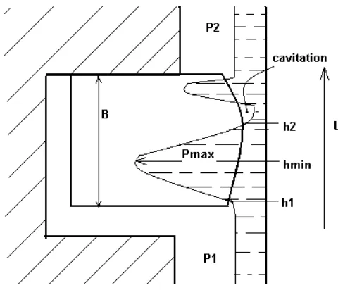
Hydrodynamic film along the width of the ring face divided into three regions first is hydrodynamic film in converging region where pressure reaches to maximum level, second is cavitation region where pressure assumes to be at atmospheric pressure and finally the third region is reformation of film above atmospheric pressure. These three zones are also represented by Mufti et.al [7].

Figure 9. Schematic of hydrodynamic oil film between liner and piston, assuming liner is moving

In figure 9, h1 is the film thickness at the entrance, hmin is the film thickness corresponding to the maximum pressure, h2 is the film thickness at the start of cavitation region and B is the width of the ring, U is the velocity of the liner in x direction. P1 and P2 are the pressure at entrance and exit of ring face.

Hydrodynamic pressure distribution of oil film along x direction in the first region can be calculated by integrating equation (2).

dP1/dx = 6ηU/h2+12ηx/h3(dh/dt)+C1/h3 (3)

27 | P a g e

qx = -h3/12η(∂P/∂x)+Uh/2 (4)

It is understood that pressure gradient at cavitation region will be zero, so flow rate at cavitation is given by;

qxcav = Uh2/2 (5)

Where, h2 is the film thickness at the start of cavitation. So pressure gradient at the exit of the ring profile would be given by continuity flow equations qx= qxcav

dP2/dx = 6ηU(h-h2)/ h3 (6)

This is the pressure gradient at the exit of ring face. And now friction force between the ring and liner per unit circumferential length can be found out by

F=o∫Bη(du/dz)dx dy (7)

Integral limits are from start of film formation to the exit point along the width ‘B’ of ring face. du/dz can be calculated by taking the differential of velocity equation in the x direction;

u = (z2-zh)/2η(∂P/∂x)+ (U1- U2)z/h+U2 (8)

Where,

U1 is the velocity of ring face U2 is the velocity of liner

As we have assumed earlier that liner is moving and ring is stationary. Now let us designate U2=U at z=0 assuming no slip;

du/dz= (-h/2η)(dP/dx) - U/h (9)

So, friction force on the moving surface would be

F=∫ {(-h/2)(dP1/dx) - Uη/h}dx +∫ {(-h/2)(dP2/dx) - Uη/h}dx (10)

(First region) (third region)

28 | P a g e 3.2 JOURNAL BEARING FRICTION

Main and big end bearing are very vital component of engine and considered to be operating entirely in the hydrodynamic regime. Basic aspects of journal bearing analysis is analyze bearing load capacity, pressure distribution, friction and lubricant flow rate as a function of load, speed and any other controlling parameters. In this study only friction behavior of journal bearing as function of speed and viscosity would be presented. For analysis, first the film geometry of bearing needs to be defined as shown in figure 11 and then applying Reynolds equation to it, will yield pressure, friction, etc. ‘e’ is the eccentricity distance between OB and Os, ‘C’ is clearance (R1-R2), R1 andR2 radius of bush and shaft, ‘h’ is film thickness.

29 | P a g e

FILM GEOMETRY

Figure 11. Film geometry of the typical journal bearings

Bearings of the heavy duty engine can be assumed to be the journal bearings with narrow bearings approximations which assume the axial length of the bush to be less than the shaft diameter. Pressure gradient along the ‘y’ direction is much larger than the x direction pressure gradient (circumferential), i.e. ∂P/∂Y >>∂P/∂X as length of bush (L) is less than circumference of shaft, i.e L<<B, so Reynolds equation may be represented as follows;

∂/∂y(h3_{∂P/∂y) = 6η(Udh/dx)}

(11)

Since h≠f(y) then it can be simplified as,

d2P/dy2= 6Uη/h3(dh/dx)

Integrating once, yield Pressure gradient in y direction, integrating once again will give pressure distribution.

dP/dy = 6Uηy/h3

(dh/dx) + C1 (12)

P = 6Uηy2/2h3(dh/dx) + C1y+C2

Now applying the boundary condition, P=0 at y= ±L/2 i.e at the edge of bearing and dP/dy= 0 at y=0 i.e at the center plane of bearing where pressure is maximum, we can solve constants C1 and C2. So the pressure distribution in narrow bearing is given by

P = 3Uη/h3

30 | P a g e

Friction force can be calculated by integrating the shear stress over the bearing area. But in case of journal bearing bottom surface, the bush is stationary whereas top surface, the shaft is moving, i.e U1=U and U2=0

F = o∫Lo∫Bη(du/dz)dxdy (14)

Friction force on the moving surface i.e shaft is given by

F = o∫B (UηL/h)dx

Where h=c(1+εcosθ) and dx=Rdθ, ε=e/c is eccentricity ratio and c=R1-R2 is radial clearance, putting it in the above equation and integrating gives Friction force on shaft.

F = (2ΠηULR/c)(1/(1-ε2)0.5 (15)

Friction force is directly related to the shaft speed and viscosity of engine lubricant in the

31 | P a g e Chapter 4

ENGINE FRICTION MEASUREMENT METHODS

Common friction measurement methods are described very briefly as follows;

Measurement of FMEP from IMEP

The gross indicated mean effective pressure is obtained from ∫ 𝑝𝑑𝑣 over compression and

expansion strokes for a four stroke engine and over the whole cycle for a two-stroke engine. This requires accurate and in-phase pressure and volume data. Accurate pressure versus crank angle data must be obtained from each cylinder with a pressure transducer and crank angle indicator. Volume versus crank angle values can be calculated. Both imepg and pmep are obtained from the P-V data. By subtracting the brake mean effective pressure, the combined rubbing friction plus auxiliary requirements are obtained.

Direct Motoring Test

Direct motoring of an engine, under condition as close as possible to the firing, is another method used for estimating friction losses. Engine temperatures should be maintained as close to normal operating temperature as possible. This can be done either by heating the water and oil flows by conducting a “grab” motoring test where the engine is switched rapidly from firing to motored operation. The power required to motor the engine includes the pumping power. “Motoring” tests on a progressively disassembled engine can be used to identify the contribution that each major component of the engine makes to the total friction losses.

Willans Line

An approximate equivalent of the direct motoring test for the diesel engines is the willans line method. A plot of fuel consumption versus brake output obtained from engine tests at fixed speed is extrapolated back to zero fuel consumption. Generally, the plot has a slight curve,

32 | P a g e Morse Test

In the morse test, individual cylinders in a multicylinder engine are cut out from firing, and the reduction in brake torque is determined while maintaining the same engine speed. The remaining cylinders drive the cylinder cut out. Care must be taken to determine that the action of cutting out one cylinder does not significantly disturb the fuel or mixture flow to the others.For a 4 cylinder spark ignition (petrol engine) engine the following steps are performed:

1. The engine is started and is run at the rated speed.

2. The maximum load of the engine is calculated and is connected to the engine. The engine is now brought to its rated speed .

3. The first cylinder is cut off by shorting the spark plug .

4. Now because the cylinder is cut off the engine speed is reduced.

5. Hence the load is to be varied such that the engine comes back to its rated speed.

6. Then the first cylinder is again started and the same is repeated for all the other cylinders. The engine can be loaded using a dynamo meter (hydraulic or eddy current)

Only the first of these four methods has the potential for measuring the true friction of an operating engine. The last three methods measure the power requirements to motor the engine. The motoring losses are different from the firing losses for the following reasons;

• Only the compression pressure and not the firing pressure acts on the piston, piston rings and bearings. The lower gas loading during motoring lower the rubbing friction

33 | P a g e Chapter 5

EXPERIMENTAL DETAILS FOR DIRECT INJECTION HEAVY DUTY DIESEL

ENGINE

TEST ENGINE

Engine test to predict the friction mean effective pressure and friction Power was conducted in a four stroke, four-Cylinder, off-highway, direct injection heavy duty, diesel engine. Specification of the test engine, used for the study is given in the Table 2.

Table 2. Engine specifications for DI

ENGINE TEST BENCH DETAILS

Test engine coupled with the appropriate AC dynamometer and instrumented with fuel

consumption measurement unit, pressure sensor, angle encoder, speed sensor, temperature indicators, data acquisition system etc, is shown in the figure 12 & 13. Engine tests were conducted at two speeds and four loads for each engine lubricant, details of operating condition are given in Table 3. Pressures at each operating speed and load was recorded and IMEP (average of 18 and 30 cycle for 1000 rpm and 2000 rpm respectively) for each operating condition was computed by using a matlab programme, given in Annexure I. Friction power (FP) is then calculated by subtracting Brake power (BP) from Indicated power (IP), at each operating point for both engine lubricants.

1. Engine type Off-Highway, DI Diesel Engine

Turbocharged

2. Displacement 4399 cc

3. Compression Ratio 18.3:1

4. No. of Cylinders 4

5. Maximum Power Output 74.2 kW @ 2200 rpm

34 | P a g e

Figure 12 Test bench setup Table 3. Test operating conditions

Figure 13. Schematic representation of experimental test set-up

Operating Conditions Values

Speed (rpm) 1000 and 2000

Torque (Nm) 50, 100, 200, 300

Temperature oil (oC) 90 ± 5

35 | P a g e ENGINE LUBRICANTS

Engine lubricants used in the experimental study are as follows; Oil ‘A’ SAE 20W-50

Oil ‘B’ SAE 10W-30

Both of these engine lubricants are commercially available, complying with API CG-4 performance category level. Typical physical characteristics of both engine lubricants are shown in Table 4. Viscosity Index is a measure of the variation in kinematic viscosity due to changes in the temperature of a petroleum product. A higher viscosity index indicates a smaller decrease in kinematic viscosity with increasing temperature of the lubricant.

It is to be noted that engine oil ‘A’ SAE 20W-50 was taken as baseline engine lubricant for

friction studies. Engine lubricants were chosen in such a way that both lubricants, having same additive package but are of different viscosity grade.

Table 4. Physical characteristics of both engine lubricants

Properties Oil SAE 10W-30 Oil SAE 20W-50

Viscosity@ 40oC cst 11.0 17.5

Viscosity@100oC cst 7.2 15.3

Viscosity Index 143 125

PRESSURE SENSOR

36 | P a g e

Table 5. Pressure sensor specifications

S.No. Parameter Value

1 Pressure range 0 – 25 MPa

2 Sensitivity -15.8pC/bar

3 Linear error ±0.2FSO

4 Temperature range -50oC upto 350oC

METHODOLOGY

Test engine was tuned as per the OEM’s recommendations before start of the test

• Engine oil was drained and flushed to remove the surface active chemistry of the

previous oil.

• Initially the baseline engine oil ‘A’ SAE 20W-50 was charged into an engine for its test run and then oil ‘B’ SAE 10W-30 was used for the study. For each engine lubricant, new oil filter was used and the test was run for three times for each engine lubricant.

• Indicated mean effective pressure (IMEP) measurements (average of 18 power cycle for 1000 rpm and 30 power cycle for 2000 rpm) was done for calculating the FMEP and also friction power at all the test operating conditions mentioned above.

• Engine oil and coolant temperatures were controlled within the range of 90oC ± 5 and 85 o

C to 90 oC respectively at all test points

37 | P a g e 5.1 RESULTS AND DISCUSSIONS

Indicated Mean Effective Pressures (IMEP) at different loads and speeds for both engine lubricants were measured from the experimental setup. Brake Mean Effective Pressure (BMEP) was calculated from the measured value of the engine brake power obtained from the engine dynamometer, by using the following relation;

Brake Power = BMEP*Vd*N/K

Where, Vd Engine displacement

N Engine revolution per minute

K = 2 for 4-Stroke engine 1 for 2-stroke engine

FMEP was calculated by taking difference of IMEP and BMEP. Mean effective pressures, test results were tabulated and represented in Table 6 and 7 for both oils at different torque and speeds. Indicated power from IMEP, Brake power measured from engine dynamometer and Friction power for both engine lubricants at different torque points and speeds were calculated and tabulated in Table 8.

Graphical representation of the variation of these mean effective pressures with different torque points at speeds (1000 rpm and 2000 rpm) for both engine lubricants are given in figure 14 and 15. Comparison of Friction mean effective pressure, FMEP and Friction power versus torque for both engine lubricants are shown in figure 16 and 17.

Table 6. Mean effective Pressures at different load for engine lubricant SAE 20W-50 at both speeds

Torque (Nm)

IMEP BMEP FMEP

1000 (rpm) 2000 (rpm) 1000 (rpm) 2000 (rpm) 1000 (rpm) 2000 (rpm)

50 2.00 2.85 1.42 1.44 0.57 1.41

100 3.21 4.29 2.86 2.86 0.36 1.43

200 6.21 6.90 5.71 5.70 0.50 1.20

38 | P a g e

Figure 14. Graphical representation of variation of mean effective pressures with load (Nm) for engine lubricant SAE 20W50 at both speed

Table 7. Mean effective Pressures at different load for engine lubricant SAE 10W-30 at both speeds

Torque (Nm)

IMEP BMEP FMEP

1000 (rpm) 2000 (rpm) 1000 (rpm) 2000 (rpm) 1000 (rpm) 2000 (rpm)

50 2.12 2.79 1.43 1.43 0.69 1.36

100 3.38 4.24 2.87 2.86 0.51 1.39

200 6.25 6.66 5.72 5.71 0.52 0.96

300 9.34 9.31 8.57 8.59 0.77 0.72

0.00 1.00 2.00 3.00 4.00 5.00 6.00 7.00 8.00 9.00 10.00

50 100 200 300

39 | P a g e

Figure 15. Graphical representation of variation of mean effective pressures with load for engine lubricant SAE 10W-30 at both speed

It has been observed from the friction mean effective pressures results that, there is significant rise in engine friction mean effective pressure with the increase in engine speed (rpm) at all load points for both engine lubricants, which indicates that speed is one of the most important factors influencing the engine friction. Other parameters on which engine friction depend are engine load, oil viscosity, oil temperatures etc. Since the oil temperature was controlled (90±5oC) for both engine lubricants, hence the effect of engine lubricant temperature

on friction can be ignored.

0.00 1.00 2.00 3.00 4.00 5.00 6.00 7.00 8.00 9.00 10.00

0 50 100 150 200 250 300

Me

an e

ffe

ct

iv

e pr

es

sr

e,

ba

r

Torque Nm Imep_1000

Imep_2000

Bmep_1000

Bmep_2000

Fmep_1000

40 | P a g e

Table 8. Indicated power (IP), Brake power (BP) and Friction power (FP) for both oils under prescribed engine operating conditions

Speed rpm

Torque Nm

IP (kW) BP (kW) FP (kW)

Oil A Oil B Oil A Oil B Oil A Oil B

1000 50 7.31 7.76 5.22 5.24 2.09 2.52

1000 100 11.78 12.38 10.46 10.51 1.32 1.87

1000 200 22.75 22.87 20.91 20.96 1.84 1.91

1000 300 34.58 34.24 31.42 31.41 3.16 2.83

2000 50 20.89 20.44 10.55 10.49 10.34 9.95

2000 100 31.48 31.12 20.98 20.94 10.50 10.18

2000 200 50.60 48.85 41.78 41.83 8.83 7.02

2000 300 68.81 68.20 62.83 62.95 5.98 5.25

Figure 16. Comparison of Friction mean effective pressure, FMEP vs torque for both engine lubricants 0.00 0.20 0.40 0.60 0.80 1.00 1.20 1.40 1.60

0 100 200 300 400

41 | P a g e

Figure 17. Engine friction power at different operating conditions for both oils

Main focus of this study is to understand the effect of engine lubricant’s viscosity on engine friction and fuel consumption. It’s a known fact that hydrodynamic friction is strongly influenced by viscosity of the lubricant and piston ring assembly and bearings are predominantly operating in these regime during the engine operation at high speed. Also, these are the major contributor in friction power loss as discussed in the introduction chapter; focus of our discussion would be restricted to establish relation between hydrodynamic friction with viscosity and other engine operating parameters.

Figure 16 and 17 shows the variation of FMEP and friction power with respect to torque at speeds (1000 rpm and 2000 rpm) for both engine lubricants. At high speed and low load, simulating the hydrodynamic lubrication conditions (prevalent in piston ring assembly and bearings), engine friction power is significantly higher as compared to the low speed and low load. This may be illustrated with the following relations showing a strong dependence of

hydrodynamic friction power on speed and oil viscosity;

It is assumed that piston rings-liner pair is operating in hydrodynamic lubrication regime at high

engine speed during mid stroke region. Hence the governing equation for piston ring/liner could be Reynolds equation. Full Reynolds equation [10] in three dimensional form, for any bearing would be;

∂/∂x(h3_∂

P/∂x) + ∂/∂y(h3∂P/∂y)= 6η (Udh/dx + Vdh/dy) + 12η dh/dt 0.00 2.00 4.00 6.00 8.00 10.00 12.00

50 100 200 300

Torque (Nm) F ri c ti o n p o w e r ( K W)

42 | P a g e

Simplifying this equation for piston ring, by assuming an infinitely long bearing, very small width as compared to the circumferential length, pressure gradient in circumferential direction can be neglected i.e ∂P/∂y=0, also neglecting squeeze at TDC. And also velocity in y direction is assumed to be zero i.e V=0 and U is piston velocity. Reynolds equation would be as follows;

∂/∂x(h3_∂

P/∂x) = 6η(Udh/dx) 16

Hydrodynamic pressure distribution of oil film along x direction can be calculated by integrating the above equation.

dP/dx = 6ηU/h2

+ C1

The minimum oil film thickness can be related to the piston velocity by following relationship

h ~ [6ηU/ (dP/dx)]1/2

17

It is also known from the above Reynolds equation that frictional force for this pair is proportional to the sliding velocity and viscosity of oil as follows;

F~ (Uη/h) 18

Combining eq. 17 and 18, it may be seen that frictional power loss (FP) for hydrodynamic lubrication conditions related with piston speed and viscosity as follows;

FP ~ η1/2

U3/2 19

For journal bearings, under light loaded conditions, Petroff equation [10] suggested that the friction power loss would vary linearly with lubricant viscosity and square of angular speed.

F = 2πηω2

LR3 / c

43 | P a g e

It may be inferred from the above discussion that speed of sliding pair is the main parameter, by which FMEP or friction power is strongly influenced. It may be observed from figure 16 and 17 that friction power/FMEP for lubricant SAE 10W-30 at high engine speed (2000 rpm) was lower than the SAE 20W-50 for all load/torque points. It may be interpreted that by using a lower viscosity grade engine lubricant at high speed, there is reduction in engine friction power/FMEP which was also corroborated by the bsfc (g/kWh) results as shown in Table 9.

At high speed, high load, the friction power is reduced to a level comparable to that of the low speed, high load condition; this may be explained with the help of well known fact that the contribution of friction as a percentage of indicated power output reduces as load increases, indicated in the figure 16 and 17 for high speed (2000 rpm) case. It may also be deciphered that

shearing of the oil film’s sub-layers would be easier at high speed and high load which helps in friction reduction, emanated due to shearing resistance in hydrodynamic lubrication conditions. At low speed, for all load levels (engine operating in boundary and mixed lubrication regime), it is observed that there is marginal change in engine friction for both oils.

It has been observed from FMEP (bar) and friction power (FP) graphs that the friction power is lower for speed (1000 rpm) as compared to the friction at high speed (2000 rpm). At low speed and high load, it may be assumed that piston ring assembly is also operating in boundary or mixed lubrication regime for most of its operating time in addition to the valve train system (operating in boundary lubrication condition). Among the piston ring assembly pack, the highest contributor to friction in an engine cycle are the top ring around top dead centre (TDC) and oil control ring throughout the engine cycle, which are operating in boundary lubrication conditions. Whereas at low load and low speed, the contribution of top ring friction at TDC is reduced, as observed in the graphs and the main contributor towards friction would be the oil control ring as seen in the FMEP and the friction power graphs. At low speed operation it is observed that higher viscosity grade oil performed comparatively well against the low viscosity grade oil, at all load points.

Brake specific fuel consumption (bsfc) at speed of 2000 rpm at all load point of an engine for both engine lubricants were calculated. Tabulated bsfc (g/kWh) is shown in Table 9; percentage reduction in bsfc (g/kWh) with the use of lower viscosity grade lubricant was also calculated. Results indicated that, there is significant reduction of fuel consumption of an engine when lower

44 | P a g e

were also observed by the authors for gasoline driven vehicle during the chassis dynamometer study [21]

Table 9. Percentage reduction of bsfc (g/kWh) of an engine operating at 2000 rpm

Torque (Nm)

bsfc (g/kWh) %

Reduction

Oil A Oil B

50 372.27 367.30 1.33

100 275.22 269.74 1.99

200 259.26 256.65 1.01

45 | P a g e Chapter 6

EXPERIMENTAL DETAILS FOR INDIRECT INJECTION LIGHT DUTY DIESEL

ENGINE

To investigate the effect of engine lubricant viscosity on fuel economy, another small experimental study was carried out on 4-stroke, 4 cylinder, indirect injection diesel engine coupled with the appropriate eddy current dynamometer and instrumented to measure the fuel consumption, power/torque etc.

TEST ENGINE

Tests were conducted on a four stroke, four-Cylinder, indirect injection diesel engine. Specification of the test engine, used for the study is given in the Table 10.

Table 10: Test engine specification for IDI

TEST ENGINE LUBRICANTS

Test engine lubricants used in the experimental study are as follows;

Oil ‘C’ SAE 15W-40

Oil ‘D’ SAE 5W-30.

Both oils were complying with API CF-4 level performance category. It is to be noted that recommended engine oil C was taken as baseline lubricant for fuel consumption studies.

EXPERIMENTAL SET UP

Test engine coupled with the appropriate eddy current dynamometer ECB 200; instrumented with fuel consumption measurement unit, power/torque measurement system etc. Fuel

1. Engine type Multi-cylinder, IDI Diesel Engine

2. Model Euro II

3. Piston Displacement 1405 cc

4. Compression Ratio 22:1

5. No. of Cylinders 4

6. Maximum Power Output 53.5 hp @ 5000 rpm

46 | P a g e

consumption was measured by using AVL 733 S fuel measurement unit with least count and accuracy of 0.001 Kg/h and 0.12% respectively.

METHODOLOGY

FUEL ECONOMY EVALUATION

• Installation of test bench comprising of diesel engine coupled with the

appropriate engine dynamometer and instrumented with various measuring equipments.

• Induction run and Baseline engine Performance (M1): Induction run on test

engine charged with Oil ‘C’ was conducted for 20 hrs as per the test cycle given in the Table 11.

• After completion of induction run, the baseline engine performance (M1) at

full load, including fuel consumption measurement was taken at following speed points; 40%, 60%, 80% and 100% of rated speed.

• After completion of the performance (M1) of engine charged with Oil ‘C’, engine was flushed with the high detergency flushing oil.

• Oil ‘D’ was charged for conducting the Induction run of 20 hrs as per the test cycle given in the Table 11 and final performance (M2) at full load, including fuel consumption measurement was taken at following speed points; 40%, 60%, 80% and 100% of rated speed.

The fuel consumption was expressed as the average of three consecutive reading at each steady

state conditions, during M1 and M2. The average bsfc in (g/kWh) at M1 (average of four averaged test points) and M2 (average of four averaged test points), was used to determine the fuel economy benefits as given below:

100 X (Avg. M1- Avg. M2) % FE = ---

Avg. M1

FE: Fuel efficiency at steady state

47 | P a g e

Table 11: Induction Run Test cycle [22]

Induction cycle

Duration(min.) Speed Load

10 Idle -

50 60% of rated speed 75%

30 80% of rated speed 100%

30 100% of rated speed 50%

6.1 RESULTS

Engine performance results at full load, for both engine lubricants are given in the Table 12 and 13. Comparative results of brake specific fuel consumption bsfc (g/kWh) for both engine lubricants at various speeds are given in Table 14. Graphical representation of comparative performance characteristics curves (Torque, Power and bsfc with respect to the speed of the engine) are provided in figure 18.

Brake specific fuel consumption (bsfc, g/kWh) calculations revealed that there is significant improvement in fuel efficiency, when lower viscosity grade engine oil ‘D’ (SAE 5W-30) was used in the engine as compared to the baseline oil ‘C’ (SAE 15W-40). Graphical representation of the comparative results is shown in figure 19. Calculations of Percentage Fuel Efficiency (%FE) show 2.18% improvement for engine charged with the low viscosity oil i.e, SAE 5W-30.

Table 12. Test results of full load Performance of engine charged with Engine Oil ‘C’

Speed (rpm) Torque (N.m) Fuel Consumption (Kg/h) Power (kW) bsfc (g/kWh) Oil temp (oC) Water out temp (oC) Air in (Kg/h)

2000 72.65 4.63 15.21 304.70 77 69 102.27

2500 74.60 5.88 19.52 301.45 87 76 128.25

3000 77.05 7.04 24.19 291.11 91 78 158.20

3500 76.25 8.07 27.93 289.04 98 80 186.02

4000 74.73 9.46 31.28 302.41 112 81 215.73

4500 71.70 10.16 33.77 298.85 125 82 241.14

48 | P a g e

Table 13. Test results of full load Performance of engine charged with Engine Oil ‘D’

Table 14: Comparative results of bsfc (g/kWh) for both engine lubricants at different speeds under steady state conditions

Speed (rpm) Oil C bsfc (g/kWh) Oil D bsfc (g/kWh)

2000 304.70 309.17

2500 301.45 294.70

3000 291.11 285.77

3500 289.04 285.47

4000 302.41 293.67

4500 300.94 299.41

5000 337.29 319.95

Speed (rpm) Torque (Nm) Fuel Consumption (kg/hr) Power ( kW )

bsfc (g/ kW.h) Oil temp (oC) Water out temp (oC) Air in (Kg/hr)

2000 73.27 4.74 15.34 309.17 80 68 106.69

2500 76.69 5.91 20.07 294.70 88 77 136.57

3000 79.47 7.13 24.95 285.77 90 75 164.22

3500 78.17 8.17 28.64 285.47 98 76 196.04

4000 77.72 9.56 32.54 293.67 106 76 228.75

4500 74.24 10.47 34.97 299.41 111 76 252.72

49 | P a g e

Figure 18. Comparative Performance characteristics curves for both engine oils

Figure 19. Comparative bsfc (g/kWh) of Oil C and Oil D

280.00 290.00 300.00 310.00 320.00 330.00 340.00

2000 2500 3000 3500 4000 4500 5000

Speed (rpm)

bsfc (g/kWh) Oil C Oil D

10 15 20 25 30 35 40

2000 2500 3000 3500 4000 4500 5000

Speed (rpm)

Power (KW) Oil C Oil D

60 65 70 75 80 85 90

2000 2500 3000 3500 4000 4500 5000

Speed (rpm)

50 | P a g e Chapter 7

ANALYSIS OF DOMINANT FACTOR INFLUENCING FRICTION POWER BY DOE

To understand the effect of various operating parameters and other factors, varying simultaneously, on engine friction characteristics a simple full factorial experimental design was used. Statistical Design of Experiment (DOE) is an efficient tool for optimizing the variables in such a way that response variables yield the desired results. A full factorial DOE, with three factors (speed, load and engine oil viscosity) each having two levels (low and high), was used for investigating the most dominant among three factors which influence engine friction significantly with 95% confidence level. The number of replicates was chosen as two and a total of 16 experiments were performed. Table 15 gives the details of factors and setting of factor

levels and Table 16 gives the typical viscosity values for the engine lubricants used for investigations.

Table 15. Factors with its levels of experiment

Factors Low Setting High Setting

Speed (A) 1000 rpm 2000rpm

Load (B) 50 Nm 350 Nm

Oil type (C ) SAE 10W-30 SAE 15W-40

Table 16. Physical properties of both engine lubricants

Properties Oil SAE 10W-30 Oil SAE15W-40

Viscosity@ 40oC cst 11.0 14.5

Viscosity@100oC cst 7.2 11.0

Viscosity Index 143 137

RESULTS AND DISCUSSIONS

51 | P a g e

in controlled conditions for both engine lubricants, hence the effect of engine lubricant temperature may be neglected as both lubricants were tested under identical conditions.

It may be observed from the results (Table 17) that the friction power of an engine charged with engine lubricant SAE10W-30 increases approximately 5 times with the increase in engine speed from 1000 rpm to 2000 rpm although load was kept constant at 50 Nm for both speed points (run order 1 & 5). Same is true for an engine charged with other engine lubricant SAE15W-40 (refer run order 2 & 16). So it may be deciphered from the above results that at high speed and low load, simulating the hydrodynamic lubrication conditions, engine friction power is significantly influenced by the speed of an engine.

Engine load also play a vital role in engine friction. With the increase in load from 50Nm to 350

Nm at high speed, 2000 rpm there is reduction in friction power for both engine lubricants, SAE 10W-30 and SAE 15W-40 (refer run order 1 & 3, 2 & 6). This may be explained with the help of well known fact that the contribution of friction as a percentage of indicated power output reduces as load increases. Also the shearing of the oil film’s sub-layers would be easier at high speed and high load which helps in friction reduction, emanated due to shearing resistance in hydrodynamic lubrication conditions. At low speed, 1000 rpm and for both load levels 50 and 350 Nm, there is marginal change in engine friction (run order 7 & 12). Also it may be observed that at high speed, high load i.e 2000 rpm & 350 Nm, the friction power is reduced to a level comparable to that of the low speed, high load condition i.e 1000 rpm & 350 Nm (refer run order 3 & 4). It was assumed that at low speed engine operates in boundary and mixed lubrication regime and with the increase in speed of an engine there is significant increase in friction power. Test results also illustrate that at high speed and low load condition, engine lubricant viscosity plays a vital role in influencing engine friction (run order 1 & 2, 9 &14), assumed to be operating in hydrodynamic lubrication regime, which indicates approximately 20% reduction in friction. So it may be concluded that, there is a reduction in engine friction when lower viscosity grade engine lubricant (SAE 10W-30) was used instead of higher viscosity grade lubricant (SAE15W-40) for engine running at higher speeds.

52 | P a g e

Analyzing the factorial design for the dominant factor with 95% confidence level, a factorial fit was used which includes main effects, first order interactions and second order interactions with estimated coefficient given in Annexure II.

Table 17. Full Factorial Design of Experiment with Response Variable Friction Power (FP), kW

Run

Order

Speed

(rpm)

Load

(Nm)

Oil

Type

Response

FP(kW)

1 2000 50 10w30 10.34

2 2000 50 15w40 12.17

3 2000 350 10w30 2.5

4 1000 350 10w30 2.56

5 1000 50 10w30 2.09

6 2000 350 15w40 2.67

7 1000 350 10w30 2.23

8 1000 350 15w40 2.85

9 2000 50 15w40 12.78

10 2000 350 15w40 4.6

11 1000 50 15w40 1.77

12 1000 50 10w30 2.1

13 2000 350 10w30 2.83

14 2000 50 10w30 10.04

15 1000 350 15w40 2.12

16 1000 50 15w40 2.08

53 | P a g e

Table 18. Estimated effects coefficients with p-values.

Factors Effects Coeff P-values

Constant 4.733 0.000

speed (A) 5.016 2.508 0.000

load (B) -3.876 -1.938 0.000

Vis (C) 0.794 0.397 0.022

speed*load (AB) -4.306 -2.153 0.000

speed*Vis (AC) 0.834 0.417 0.017

Friction Power (FP) = 4.733+2.508A – 1.938B+ 0.397C - 2.153 A*B + 0.417 A*C

It can be seen from the Table 18 that engine friction power increases with the increasing speed (5.016) and engine lubricant viscosity (0.794). But friction power response decreases with the increase in the load of a fired engine (-3.876), which is true, as the percentage contribution of friction power of a fired engine is very less as compared to the power output at high loads. To identify and screen the active factors (effects) which influence the response, friction power significantly, normal probability plot and Pareto chart were used. In figure 20, the normal plot of the all factors; main effects, first order interaction and second order interaction points were plotted. It can be inferred that points that do not fit the line well, usually signal active effects. Active effects are larger and farther from the fitted line. In our case factors A, B, AB, C, and AC are considered to be the significant factors.

A Pareto chart of the effects is another tool, shown in figure 21, which is very much useful in determining the active effects. It also indicated the active effects, same as observed in the normal plot. Both normal plot and Pareto chart uses the same value of α = 0.05 for determining significance of effects with 95% confidence level.