ANN Based Model for Predicting RF Signal Received Power in Indoor Propagation Links

2016 International Conference on Mathematical, Computational and Statistical Sciences and Engineering (MCSSE 2016) ISBN: 978-1-60595-396-0

ANN-Based Model for Predicting RF Signal Received

Power in Indoor Propagation Links

Juan Antonio ROMO ARGOTA and Ignacio ANITZINE

Department of Communication Engineering, University of The Basque Country, Bilbao, Spain

Keywords: Artificial neural networks, Neuron model, Learning rules, Backpropagation, Mobile communications, Ray-tracing, Dominant path.

Abstract. This chapter presents the use of Artificial Neural Networks (ANN) to predict the received power/path loss in indoor links. The prediction approach combines the use of ANNs and ray-tracing in order to identify and parameterize the so-called dominant path. A complete description of the process for creating and training an ANN-based model is presented, in which past values of one or more time series are used to predict future values. Special emphasis is placed on the training process. More specifically, we will be discussing various techniques to arrive at valid predictions focusing on an optimum selection of the training set. A quantitative analysis based on results from narrowband measurement campaigns is also presented.

Introduction and Prediction models

The need for connectivity anywhere, added to the increment in the number of users, has triggered the development of various generations of mobile communication standards in the last decades. Accurate and fast prediction models are needed for making received signal level/path loss predictions prior to actual network deployment. In this paper we analyze the performance achievable with an intermediate technique between purely empirical and purely deterministic, based on the use of Artificial Neural Networks, ANNs.

A great variety of methods has been proposed for predicting the expected received electric field level or, alternatively, the path loss. These calculations can be made using empirical or deterministic models. An intermediate alternative is using artificial neural network-based (ANN) models.

Empirical models are based on measurement campaigns carried out in specific, representative environments. Regression techniques are then used for obtaining mathematical expressions describing the propagation loss as a function of the path length. The computational efficiency of these models is satisfactory, while having a limited accuracy. A typical example is the well known Okumura-Hata model [1].

On the other hand, deterministic models apply accurate electromagnetic techniques or simplified versions of them. These require accurate input information of the propagation environment: buildings, etc. Their main advantage is their precision, despite their lack of computational efficiency. It is quite common to see high frequency approximations of the full wave solutions which make use of ray-tracing techniques for identifying all possible paths between the transmitter and the receiver including multiple reflections, diffractions and transmissions through walls. The contribution of each ray is then calculated by using Fresnel's transmission and reflection coefficients, and GTD/UTD for diffracted contributions.

ANN-base models try to combine the advantages of empirical and deterministic models. In the literature, the most common choice is using feedforward networks, commonly referred to as multilayer perceptrons (MLPs). An alternative is to use the so-called radial basis function networks (RBF) for their fast convergence, robustness and small size [2].

that the generalization properties of ANNs may be reduced, i.e., they may be more sensitive to the training set data [3].

In the hidden layers, non-linear activation functions are normally used, e.g., sigmoid-type functions. For the output level, linear functions are normally used. In the hidden layers, also wavelet functions can be found in received field prediction applications [4]. However, even though they show faster computation times, in contrast, they require much larger training data sets.

Different algorithms can be used for training an ANN. In [5] their efficiencies were analyzed showing that the best results are obtained with Bayesian Regularization and Levenberg-Marquardt techniques, the latter being the most used option. Another algorithm also used offers good performances is the Resilient Propagation algorithm.ANNs can also be combined with other techniques for characterizing the effects of RF propagation. When simulation time is critical, the so-called "dominant path", selected by means of a ray-tracing tool, can be used to provide the necessary inputs to the AAN. This leads to acceptable results both in terms of time and accuracy. The dominant path is the propagation path between the transmitter and receiver showing the smallest loss. Thus, instead of searching for all possible ray combinations, the problem is simplified while an acceptable generalization performance may be achieved. The dominant path can be calculated using two main techniques: the recursive neighboring model and the convex corners approach [6].

In last few years, many researchers have applied ANNs for predicting path loss in indoor environments [7].

Data Collection and Preprocessing

A single transmitter is assumed while various receive locations can be defined as part of a route or a meshed grid. The route option is very well suited for the training process.A continuous wave, CW, transmitter was set up at a number of sites while the received power was measured at several points along a number of routes. Measurements were repeated several times so as to average out the signal cancellations and enhancements due to multipath. For each measurement point, information on its coordinates and the received power level in dBm were recorded. All the measurement routes and the transmit locations are shown in Figures 1. CW measurements were made at the 900 and 1800 MHz bands, using a vertically polarized 4 dBi gain antenna and 35 dBm transmit power. Receiver was a spectrum analyzer connected to a PC. Measurements were triggered every 350 cm along the route. Receive antennas were also vertically polarized, with onmidirectional patterns and 0 dBi gains.

Figure 1. Indoor measurement routes and transmitters.

Selecting the Architecture

Starting from an earlier version of the tool [7], we have implemented a new one using the dominant path approach. Then, this implementation has been trained with measurements. Finally, comparisons between predictions and measurements for data sets different from those used for training were carried out.

ANN is a MLP network with pyramidal structure consisting of three main parts: an input layer with 8 neurons, each associated with one of the 8 selected input parameters, two hidden layers with 6 and 4 neurons, respectively, with sigmoid-type activation functions and, finally, an output layer with a single neuron with a linear function (Figure 2).

Figure 2. Architecture of the neural network.

Input parameters must characterize the propagation path between transmitter and receiver:

- Screen effect, Po1, Po2. It occurs when there are walls near the transmitter or receiver blocking the direct ray.

- Local reflections, Po3, Po4. They exist when either the receiver or the transmitter are located close to a corner giving rise to multiple reflections.

- Waveguide effect, Po5. It appears in corridors.

- Change of direction, Po6. It occurs when diffraction takes place.

- Transmission loss, Po7. It is introduced when the signal must pass through an obstacle. - Free space loss, Po8. It depends on the distance and the frequency.

The most critical step when designing an ANN-based model is the training process. The back-propagation technique was selected as learning method, where the predicted power is compared with the actual measurement and the difference (error) is fed back to the network for correcting the various network connection weights. The Levenberg-Marquardt algorithm was used for training the model. This method uses the evolution of the gradient changing the coefficient for each neuron connection in the direction that causes a larger error reduction. The chosen number of training cycles was one thousand. This is a tradeoff between error and time.

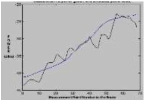
After the ANNs were trained, we analyzed the prediction errors by comparing the results of the ANN-based model and the received power levels measured at points different from those used in the training phase. Figure 3 illustrates a measurement route and the obtained prediction. For each route, the mean error, mean squared error and standard deviation were calculated. In the figure we can observe how the prediction curve is much smoother than that of the measurement. This is because the ANN input parameters, obtained from the ray-tracer, are very similar for neighboring points along the route. The user of such a prediction tool must be aware of this limitation. Still, as observed, the average error and its spread are very small.

Training the Network and Conclusions

A wise selection of real propagation paths from which the neural network will learn how to calculate the received power is the most critical factor in the training phase. Those real situations form the so-called "training set". To optimize the training set several routes with different characteristics must be selected so as to provide the ANN with all the propagation conditions (reflection paths, direct ray paths, etc.) likely to be encountered. In addition, the selected routes have to include received positions showing different ranges of input parameters. In this way, the network will learn to behave in many different situations and will be able to make correct generalizations when applied to new cases. After learning from a number of routes, the network must be tested with other data sets from different routes. Predictions for those test routes must show similar errors to those for the training routes. If this is the case, network will be correctly trained.

The first and essential step in the training process involves a suitable characterization of the measurements points in the training routes according to their dominant path type. The choice of training routes must be a planned process based supplying a sufficient and balanced number of measured points belonging to the various propagation conditions to be expected. Based on the dominant path concept, we have to be careful when training the ANN to provide an appropriate mix of the four path types identified.

A total of 50 measurement routes were recorded, each with a different number of receive positions depending on its length. Hence, the available measurements correspond to a total of 79 routes with 3420 sampling or receive points. As indicated earlier, each route was measured several times and, then, point-wise averages were calculated. The number of transmitter sites was 6 while. Table 1 presents a summary of all measurement locations according to their corresponding path types.

Table 1. Classification of receive locations and Distribution of measurement points in Sets-A and –B.

Indoor receivers % of total Set A Set B

LOS direct ray 572 16.7 399 406

NLOS reflection - - 30 101

NLOS diffraction 635 18.6 219 390

NLOS obstacles 2213 64.7 648 (17.5% of 3420) 897 ( 26% of 3420)

TOTAL 3420 100 Set A Set B

Two strategies have been analyzed in the selection of the training set. In the first we selected entire routes while the second focused on selecting specific receive points according to the dominant path category to which they belonged.

We now analyze the first, i.e., route-wise strategy. From the available measurements, a subset of the routes was used for training while the rest was used for testing. To illustrate the effect of the number of routes considered in the training process in relation to the achieved prediction accuracy, several training sets were used as discussed below.

3420). The distribution of path types is as follows: 406 were direct ray paths, 101 diffraction paths and 390 through-obstacle paths, Table 1. For the test set four complete routes were used, Table 2.

Table 2. Numerical results of simulations, with two and four transmitters.

Test routes Route 6 Route 7 Route 8 Route 9 Network trained with Set-A

Mean error 1.23 2.58 2.19 2.37

RMS error 1.72 3.46 3.14 3.27

std 1.20 2.31 2.25 2.25

Network trained with Set-B

Mean error 0.96 1.99 1.36 1.47

RMS error 1.48 2.84 1.99 2.60

std 1.13 2.03 1.45 2.15

In the case of Set-B, the errors were much smaller than for the Set-A. With the new training, the same routes were simulated. Due to the path type mix in Set-A, routes with diffraction paths were badly predicted: the network so trained cannot properly simulate those measurement points where the dominating conditions are not sufficiently well represented in the training set. Training Set-B introduces more measurements and also covers a more balanced mix of propagation path types. Thus, the selected routes in Set-B encompass an appropriate assortment of paths from all types.

Now we analyze the second strategy to selecting the training set, i.e., a path-type oriented selection. In this case, the training process was separately carried out for each type of propagation path. Training the ANN with separate receiver locations according to their propagation path types could, in principle, allow achieving a much better prediction accuracy. According to this approach, several routes were split into subsets, as a function of their dominant path, so that all receive points with a direct-ray predominant path were placed into the same subset. Then, some of those points were used to train the ANN and others for testing it.

As shown in Table 3, results show a similar error parameter range. The error parameter range in through-obstacle and diffraction paths is in the order of 2-3 dB, whereas for direct ray paths it again shows a lower value. In any case, the general performance is quite good, it does not seem to be much better than the one achieved in the previous analyses.

Table 3. Errors for the path-type oriented analysis for the indoor case.

Test routes LOS direct ray NLOS diffraction NLOS obstacles

Mean error 1.77 3.26 2.15

RMS error 2.52 4.74 3.15

std 1.79 3.44 2.30

References

[1] M. Hata, Empirical formula for propagation loss in land mobile radio services. IEEE Trans. Veh. Tech., 29 (3) (1980), 317-325.

[2] Y. Sun, Y. Xu and L. Ma, The Implementation of Fuzzy RBF Neural Network on Indoor Location, Proceedings of the Pacific Asia Conference on Knowledge and Software Engineering, 2009.

[3] E. Östlin, H.J. Zepernick and H.Suzuki, Macrocell Path-Loss Predicition Using Artificial Neural Networks, IEEE Transactions on Vehicular Technology, vol. 59, no. 6, July 2010.

[4] Fang Cheng and Huairong Shen, Field Strength Prediction Based on Wavelet Neural Network, 2nd International Conference on Education Technology and Computer (ICETC), 2010.

[6] G. Wölfle and F.M. Landstorfer, Dominant Paths for the field strength prediction, 48th IEEE Vehicular Technology Conference, Ottawa, Ontario, Canada, vol. 1, pp. 552 – 556, May 1998.