2017 International Conference on Computer, Electronics and Communication Engineering (CECE 2017) ISBN: 978-1-60595-476-9
Binary Classification on ECoG Signals Using Optimized
Extremely Learning Machine
Xin-man ZHANG
1, Yi-xuan DAI
2,*,
Xue-bin XU
3and Ting-ting HE
41MOE Key Lab for Intelligent Networks and Network Security,
Xi’an Jiaotong University, Xi’an, 710049, China
2School of Electronics and Information Engineering,
Xi’an Jiaotong University, Xi’an, 710049, China
3Guangdong Xi'an Jiaotong University Academy, No. 3, Daliangdesheng
East Road, Foshan, Guangdong 528000, China
4School of Electronics and Information Engineering, Xi’an Jiaotong University, Xi’an, 710049, China
*Corresponding author
Keywords: Binary classification, ElectroCorticoGram, Optimized extreme learning machine, Superior speed.
Abstract. In order to improve the accuracy of brain signal processing and accelerate speed meanwhile, we present an optimal and intelligent method for large dataset classification application in this paper. Optimized Extreme Learning Machine (OELM) is introduced in ElectroCorticoGram (ECoG) feature classification of motor imaginary-based brain-computer interface (BCI) system, with common spatial pattern (CSP) to extract the feature. When comparing it with other conventional classification methods like SVM and ELM, we exploit several metrics to evaluate the performance of all the adopted methods objectively. The accuracy of the proposed BCI system approaches approximately 92.31% when classifying ECoG epochs into left hand little finger or tongue movement, while the highest accuracy obtained by other methods is no more than 81%, which substantiates that OELM is more efficient than SVM, ELM, etc. Moreover, the simulation results also demonstrate that OELM will significantly improve the performance with p-value being far less than 0.001. Hence, the proposed OELM is satisfactory in addressing non-stationarity of ECoG signal.
Introduction
The development of brain–computer interfaces (BCI) has undergone extensive growth in recent years, with the aim of providing an effective method for human-computer interaction without neuromuscular transmission [1]. The ultimate goal of BCI research is to establish a direct communication system that translates human intentions, which is reflected by specific brain signals, into a control command for output devices [2].
In recent years, many innovative methods are commonly used in processing binary-class ECoG signals of motor imagery. For example, support vector machine (SVM) is a supervised learning model that is used for pattern recognition, classification, and regression analysis. However, when processing training samples in large size, it is difficult to implement and can’t produce satisfactory results whether in precision or speed. Therefore, a newly different classification method named extreme learning machine (ELM) is proposed by scholar Guang-Bin Huang from Nanyang Technological University. ELM has better generalization performance and fast executing time than SVM [3].
classification accuracy and speed. Especially when processing signals in large size, it is supposed to save a lot of time.
Preliminaries
In this section, first we adopt CSP to extract features of ECoG signal, then transfer them to feature classification module, using ELM to train and test the corresponding data. Then an improved classification algorithm named Optimized Extreme Learning Machine (OELM) is proposed and put into practice on the basis of ELM. Here the basic principles of ELM and OELM are introduced. Also, the detailed process and procedure are presented.
Extreme Learning Machine
With its fast speed and high precision, Optimized Extreme Learning Machine (OELM) is more effective in discriminating two classes of ECoG data than conventional algorithms. As the basis of OELM, Extreme Learning Machine (ELM) has been paid more attention by researchers around the world in recent years. It is a neural network essentially, which is composed of input layer, hidden layer and output layer [3].
Assuming that a single-hidden layer feed-forward neural network (SLFN) is given, and it has N
hidden layer nodes. Different from the previous algorithm that all parameters need to be tuned by feed-forward neural network, ELM can accurately learn N different observation values with no need
to adjust the weights between input neurons and initial hidden layer bias in practical application [3]. In fact, many simulation results also show that ELM is not only fast in classification speed, but also can yield very high recognition accuracy. The steps of ELM are presented as follows:
Firstly, randomly given N sample pairs
( , )
x o
j j , wherex
jando
j respectively denote the input andthe output, T m
jn j
j j
j
x
x
x
x
R
x
[
1,
2,
3,
...
,
]
,o
j
[
o
j1,
o
j2,
o
j3,
...
,
o
jl]
T
R
l. Given the number ofhidden layer nodes in the network is N~ , and activation function is set to g x
, then the corresponding SLFN is expressed as follow:~ ~
1 1
( ) ( ) 1 , 2 ,... , .
N N
i i j i i j i j
i i
g x g a x b o j N
(1)where T
im i
i
i
[
1,
2,
...
,
]
. It is the weight between the ith hidden neurons and the mth outputneurons; while T in i
i
i
a
a
a
a
[
1,
2,
...
,
]
, it represents the weight of each input neuron to the ith hiddenneuron;
a
i
x
j is inner product of them; biis threshold of the ith hidden neuron;o
j is value of the jth output neuron. The selection of activation function is not unique.All the equations above can be written compactly as formula (2) shows:
.
H T (2)
Assuming that E(W) is the sum of the squared error between the desired output and the actual
output of neural network, target optimization remains to be a problem: That is to find an optimal weight valueW (a,b,), which makes E(W) takes the minimum value [4]. The following mathematical model is established:
~
2 ( , , ) ( , , )
1
arg min ( ) arg min
. . ( ) .
W a b W a b
N
i i j i j j
i
E W
s t g a x b t
(3) where
j
[
j1,
j2,
,
jm]
, and it represents the deviation of the jth output sample.When H in formula (2) is unknown, adjust weight W as follows:
W W E W
Wk k
) ( 1 (4)
The equation ( ) 1 ()( )
1 ) ( p i l N p P N i l d b g d b
g
holds only when the activation function g(x) isunlimited.
Thus weight of the output layer can be directly solved by the least square method. Since ELM has no need of iteration, the learning speed is much faster than traditional classification algorithms. By continuously adjusting numbers of hidden layer node, the learning ability and classification accuracy can both achieve an optimal value [4].
Optimized Extreme Learning Machine
Although ELM outperforms SVM in both classification speed and accuracy, it is very unstable when processing high dimensional but small samples, which results from the random assignment of input weights. Therefore, we proposed an improved algorithm based on ELM, which is called Optimized Extreme Learning Machine (OELM), where projection of feature signal is introduced, and we use the singular value decomposition (SVD) to assign a value to input layer. Steps of OELM are presented as follow at the basis of ELM:
Firstly, the characteristic of input signal is represented by matrix XNm , where N and m
respectively represent number of samples and attributes of the signal;
Secondly, do singular value decomposition (SVD) to input matrix. SVD is widely used in image processing, signal classification, pattern recognition and so on. In this experiment, SVD is represented as follows:
( ) T.
svd X PSQ (5)
where Pand Q are the left and right singular matrices of input matrixX .The singular value matrix
S is composed by singular values which are arranged in descending order. Select the d singular
vector elements in S corresponding to the largest singular values, which is used to approximate input
matrixX . Finally, the optimal rank of X is obtained as follows:
( ) .
d d d d
best X P S Q (6)
Next, in the low dimensional space composed byQd, high dimensional data is represented as
follows:
.
d d d
XQ P S (7)
Then, in order to overcome the defect of poor performance in processing high dimensional small sample, we set the input layer weights for projection vector, instead of giving random value. That is,
d
Q
W .This improvement simplifies the complexity of the network. Output of hidden layer can be obtained by formula (8) after determining input layer weights:
( d) ( d d).
H g XQ g P S (8)
where g(x) is a single hidden layer neural network transfer function.
At last, the output layer weights can be calculated by means of a linear expression as follow:
.
H T (9)
The training module is over after the above five basic steps. The deterministic assignment of input layer overcomes the defect of ELM. And result shows that classification performance of OELM is very stable.
Description of the Classification Procedure
In order to evaluate the proposed classification algorithms, data set I of BCI competition III is adopted in this study. It is provided by University of Tübingen, Germany, Dept. of Computer Engineering (Prof. Rosenstiel) and Institute of Medical Psychology and Behavioral Neurobiology (Niels Birbaumer), and etc [5]. There are 378 trials in total. Every single trial represents either an imagined tongue or finger movement and is recorded for 3 seconds duration. Among the total 378 trials, 278 labeled trials are used to train classifiers, whereas other 100 unlabeled testing trials are available for measuring generalization performance of the trained classifier. Task in this study is try to correctly classify the testing data set (100), where all these samples belong to either negative or positive class.
Based on description above, features of brain signals can be extracted by CSP at every sampling point. We adopt the extracted features to train OELM classifier in training dataset, and then the trained classifier is applied to classify the features extracted at the same sampling point in testing dataset. Firstly, we sample and collect signals from brain. In this experiment, we increase the hidden layer node by one degree from 10 to 60. Sampling points are simply set to 1500, 2000 and 2500, respectively; then CSP is applied to extract features after acquiring ECoG signals from 64 electrodes; at last, 16 different activation functions are chosen to OELM for classification. All experiments are performed on several sets of parameters with 278 trials to train OELM and the remaining 100 to test performance of the trained OELM.
Experiment Results and Discussion
We conduct all experiments under the exactly same development environment. Experiments are performed on the same computer with Intel core i3 2 processor 2.4GHZ with 4 GB memory and implemented by MATLAB 7.12(2011a, 64bit). In the following section, results of the mentioned methods are presented and discussed.
Preprocessing Stage
[image:5.612.112.503.64.223.2]
(a) trial 9 (b) trial 10
Figure 1. Relative amplitude contribution of (a) and (b). Black dots denotes 64 channels, and each color bar represents the range of signal voltage.
As is shown in Figure 1, trial 9 and 10 have rather different contour line distribution, while region in red of (a) basically shows blue of (b), which represents low voltage potential. This strongly illustrates that CSP can extract features effectively. We can easily notice that in Figure 1, Region of Interest (ROI) is concentrated over the sensorimotor cortex area [6], where locates the 22nd, the 29th to the 32nd, and the 37th to the 40th channel. We hand-select those more discriminative channels and pick out trial 9 and 10, whose level curves have the largest difference among the other one, and plot their amplitude-sampling points curves corresponding to those nine channels, as is shown in Figure 2.
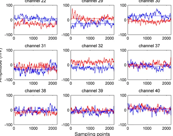
Figure 2. Amplitude of nine channels from trial 9 and 10 of training data.
In Figure 2, curves in red represent voltage of trial 9 while the blue denote that of trial 10 from raw training data. The straight lines parallel to horizontal axis show the mean values corresponding to each trial. Channels are regarded as “good” if they are visibly discriminable on average between two classes [7]. We transfer the features extracted by CSP to SVM, ELM and OELM, results are listed below.
Results on Extreme Learning Machine
[image:5.612.157.447.357.585.2]“Triangular basis” (tribas) and “Radial basis” (radbas). We list the optimal classification accuracy corresponding to specific sample point and hidden layer nodes in Table 1.
Table 1. Objective classification performance of ELM.
Parameters Evaluation metrics Activatio
n function Sample point layer nodes Hidden Classification accuracy [%] Average training time [s] Average testing time [s] sin 2000 58 80.77 0.0043 0.0012 sig 2500 32 80.77 0.0006 0.0006 hardlim 2000 50 78.21 0.0015 0.0031 tribas 2000 57 71.79 0.0015 <0.0001 radbas 2500 50 75.64 0.0012 0.0012
Table 1 gives performance of 5 activation functions based on ELM with sampling point increasing from 1500 to 2500. It is noteworthy here that the maximum of classification accuracy (80.77%) is obtained with “Sine” (sin) and “Sigmoid” (sig) function. Besides, we can also get a relatively shorter time, especially when activation function takes “sig”, the average training time and average testing time are both 0.0006 seconds. Compared with experimental results under other conditions, system performance is optimal.
However classification accuracy is still not good enough. The reasons are as follows: on the one hand, as the feature extraction method, CSP does not take the frequency domain information into account, which will generate unrepresentative ECoG features, and affect classification accuracy later [7]; on the other hand, we apply ELM in feature classification. Due to its random assignment of input weights, it is difficult to get global optimum in the process of finding the optimal weight [8]. These two points make sense as CSP combined with ELM can’t reach satisfactory results. Then, OELM is proposed and put into practice as is shown in section below.
Results on Optimized Extreme Learning Machine
[image:6.612.104.508.495.647.2]For OELM, the kinds of activation functions are up to 16. Similarly, we set sampling points to 1500, 2000 and 2500. So 48 experiments are completed and we list the optimal results under every parameter setting on Table 2 without the “Radial basis” (radbas), “Triangular basis” (tribas), “Hard limit” (hardlim), “Cosine” (cos), “CosineH” (cosh) and “arcCosineH” (acosh), whose classification accuracies are lower than 70%.
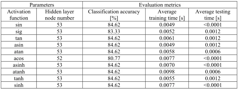
Table 2. Objective classification performance of OELM
Parameters Evaluation metrics Activation
function node number Hidden layer Classification accuracy [%] training time [s] Average Average testing time [s] sin 53 84.62 0.0049 <0.0001 sig 53 83.33 0.0052 0.0012 tan 53 84.62 0.0061 0.0012 asin 53 84.62 0.0049 0.0012 atan 53 84.62 0.0058 0.0006 acos 52 80.77 0.0077 <0.0001 asinh 53 84.62 0.0070 <0.0001 atanh 53 84.62 0.0098 0.0006
tanh 53 84.62 0.0055 0.0012 sinh 53 84.62 0.0077 <0.0001
respectively, with average training time being 0.0049 seconds and 0.0052 seconds, while average testing time being lower than 0.0001 seconds and 0.0012 seconds respectively.
It also need to be emphasized here that the activation function “sin”, g(x) =sin(x) and “sig” g(x) =S(x) =1/ (1+e^ (-x)) are used in ELM and OELM classifiers for their better performance. Since the singular value decomposition (SVD) can reduce data dimension effectively, it’s better to combine SVD with these two activation functions. This, together with a closer look at results from Table 1, suggest that “sin” and “sig” are more valuable for our binary decision tasks than others.
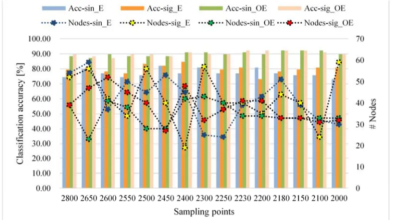
[image:7.612.111.503.230.453.2]We still expect a further improvement of classification accuracy, proper selection of sampling point and hidden layer nodes may markedly functioning [9]. We are supposed to lessen number of hidden layer nodes, which can effectively reduce the complexity of network. Figure 3 compares performance at different sampling points setting. For each case, we calculate the least number of hidden layer nodes and plot it in secondary axis.
Figure 3. Bar plot visualizes the performance corresponding to each sampling point number.
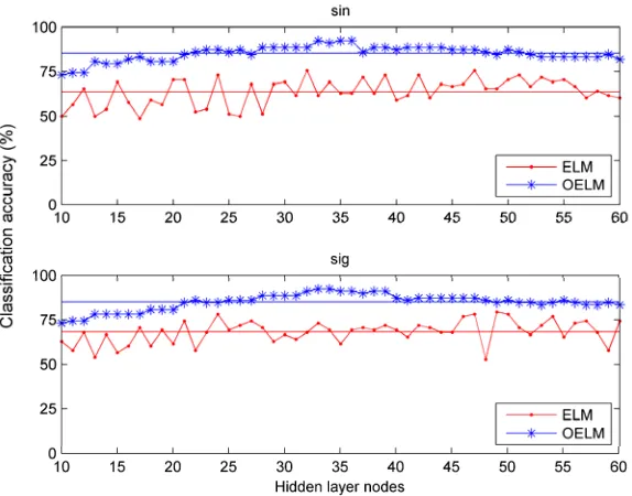
Figure 4. Classification accuracy of ELM and OELM with the same parameters.
For each activation function, different numbers of hidden layer node, ranging from 10 to 60 are applied to ELM and OELM. Thereafter, classification accuracy corresponding to each set of parameters are calculated on testing data. Tables 3 and 4 compare the performance of ELM with that of OELM, with activation functions being “sig” and “sin”.
Table 3. Performance comparison of ELM and OELM for activation function: sig.
Algorithm s
Time [s] Testing accuracy [%]
p-value H #nodes Training Testing Max Mean Std RMSE
[image:8.612.98.512.391.523.2]ELM <0.0001 <0.0001 75.64 66.26 6.07 34.61 p<0.0001 1 40 OELM <0.0001 <0.0001 92.31 84.92 4.61 15.92 33
Table 4. Performance comparison of ELM and OELM for activation function: sin.
Algorithm s
Time [s] Testing accuracy [%]
p-value H #nodes Trainin
g Testing Max Mean Std
RMSE
ELM 0.0156 <0.0001 79.49 64.88 6.80 36.11 p<0.0001 1 39 OELM 0.0312 <0.0001 92.31 85.14 4.26 15.60 33
In Tables 3 and 4, “Std” and “RMSE” mean standard deviation and means root mean square error respectively. P-value and H are obtained by t-test, which we use to compare the discrimination of classification accuracies corresponding to ELM and OELM.
[H, p] = TTEST(X, Y). (10) Formula (10) performs a paired t-test of the hypothesis, where two matched samples in vectors X and Y, come from distributions of ELM and OELM with equal means, and return result of testing in H. H=0 indicates that hypothesis ("equal means") cannot be rejected at the 5% significance level. H=1 indicates that hypothesis can be rejected at the 5% level.We set testing accuracy obtained by ELM as parameter X while that of OELM as Y in t-test function. Both results show that H equals 1, meaning two testing accuracy samples are rather different. P-values are far less than 0.0001, which indicates that mean values of the two samples equal with the probability less than 0.01%. This confirms that OELM obtains significant improvement on classification accuracy in comparison with ELM.
the increase of classification accuracy achieved by OELM are 21.97%, and 23.80% in comparison with ELM under the same condition. As observed from Tables 3 and 4, generally speaking, ELM and OELM obtain similar performance in classification speed. However, number of hidden nodes required by ELM is larger than that of OELM, meaning the complexity of OELM is much lower than ELM [10].For whether “sin” or “sig” function, the maximum and mean value of classification accuracy obtained by OELM are rather higher than those achieved by ELM. Meanwhile, the standard deviation and root mean square error of testing accuracy by OELM are lower than those by ELM.
Comparison with Other Classification Methods
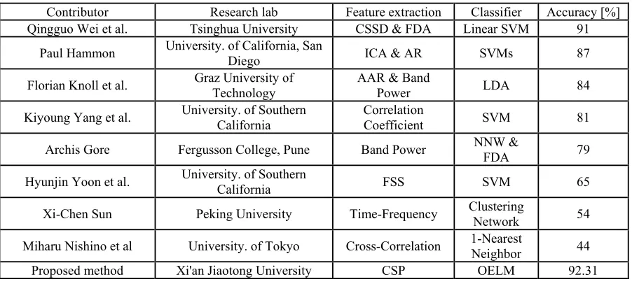
[image:9.612.82.533.243.446.2]We compare our method with those proposed in [11], which share the same dataset. Table 5 lists several experiment results, their feature extraction methods and classifiers. The last column shows the classification accuracies corresponding to each method.
Table 5. Classification results comparing the proposed method with other methods.
Contributor Research lab Feature extraction Classifier Accuracy [%] Qingguo Wei et al. Tsinghua University CSSD & FDA Linear SVM 91
Paul Hammon University. of California, San
Diego ICA & AR SVMs 87 Florian Knoll et al. Graz University of Technology AAR & Band Power LDA 84
Kiyoung Yang et al. University. of Southern California
Correlation
Coefficient SVM 81 Archis Gore Fergusson College, Pune Band Power NNW & FDA 79
Hyunjin Yoon et al. University. of Southern
California FSS SVM 65 Xi-Chen Sun Peking University Time-Frequency Clustering Network 54
Miharu Nishino et al University. of Tokyo Cross-Correlation 1-Nearest Neighbor 44 Proposed method Xi'an Jiaotong University CSP OELM 92.31
[image:9.612.81.531.541.638.2]Table 5 indicates that our method obtains an accuracy of 92.31%, which is 1.31% higher than Qingguo Wei’s method, the best of the others. It can be concluded that our BCI system outperforms those listed with CSP to extract the features and OELM to classify them afterwards. The performance of the proposed algorithm is also compared with several other classification methods listed in [11] in Table 6, which all share the same dataset and adopt CSP as the feature extraction algorithm.
Table 6. Classification results comparing the proposed method with other methods.
Contributor Research lab Feature extraction Classifier Accuracy [%] Liu Yang et al. National University of Defense Technology CSP LDA 86
Zhou Zongtan et al. National University of Defense
Technology CSP LDA 84 Bin An et al. University of Science and Technology of China CSP SVM 48 Proposed method Xi'an Jiaotong University CSP OELM 92.31
Table 6 reveals that our method obtains an accuracy of 92.31%, which is 6.31% higher than Liu Yang’s method, the best of the others. The results prove that OELM shows higher classification accuracy than SVM and LDA under condition of same feature extraction method (CSP). We also evaluate our method in terms of computation time, which includes training and testing time.
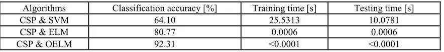
Table 7. Results of different algorithms.
Algorithms Classification accuracy [%] Training time [s] Testing time [s] CSP & SVM 64.10 25.5313 10.0781 CSP & ELM 80.77 0.0006 0.0006 CSP & OELM 92.31 <0.0001 <0.0001
As seen from Table 7, CSP combined with OELM achieves the highest accuracy, which is 11.54% higher than ordinary ELM. On the whole, OELM outperforms SVM both in accuracy and speed. Compared with accuracies obtained by SVM and ELM, accuracy of OELM is more competitive. Defects in the application of SVM can be successfully overcame by OELM for its high accuracy and fast speed. The BCI system can generate better results with OELM than with other state-of-the-art methods when analyzing and processing ECoG signals [12]. Seen from Table 7, ELM is comparable with OELM in speed, however OELM runs much fast than SVM by a factor up to thousands, whether in training or testing module. Furthermore, OELM can achieve the maximum testing rate 92.31% with 33 nodes, which is significantly higher than all the results so far listed in the ranking of the BCI competition III, using some popular algorithm such as SVM [13]. It can thus be concluded from the results displayed in these figures and tables that OELM is much more suitable and competitive for binary-class signals of motor imagery.
Conclusions
In this paper, a newly intelligent and efficient learning algorithm called Optimized Extreme Learning Machine (OELM) is presented and applied in motor imagery signals classification with CSP to extract features. The proposed method outperforms conventional popular learning algorithms for the extremely fast learning speed and good generalization performance, which is demonstrated with the BCI competition III data set I. Different sampling points and activation functions are employed in different experiments to analysis the property of OELM. The results show that OELM need less computational time and obtain better accuracy than SVM and ELM. In conclusion, OELM is the novel and efficient classifier for biometric applications. Although only binary-class classification strategy is discussed in our study, OELM can also be applied to solve multi-classification problem. We believe that this method has great potential for the design of real-time BCI systems.
Acknowledgement
This work was supported by grants from the National Natural Science Foundation (No. 61673316), the Major Science and Technology Foundation in Guangdong Province of China (No. 2015B010104002), and the Fundamental Research Funds for the Central Universities.
References
[1] Fang, Y.; Chen, M.; Zheng, X. Extracting features from phase space of eeg signals in brain–computer interfaces. Neurocomputing 2015, 151, 1477-1485.
[2] Wolpaw, J.R.; Birbaumer, N.; Heetderks, W.J.; Mcfarland, D.J.; Peckham, P.H.; Schalk, G.; Donchin, E.; Robinson, C.J.; Vaughan, T.M. Brain-computer interface technology: A review of the first international meeting. IEEE Transactions on Rehabilitation Engineering A Publication of the IEEE Engineering in Medicine & Biology Society 2000, 8, 164-173.
[3] Huang, G.B.; Ding, X.; Zhou, H. Optimization method based extreme learning machine for classification. Neurocomputing 2010, 74, 155-163.
[5] Information on http://www.bbci.de/competition/iii/.
[6] Leuthardt, E.C.; Freudenberg, Z.; Bundy, D.; Roland, J. Microscale recording from human motor cortex: Implications for minimally invasive electrocorticographic brain-computer interfaces. Neurosurgical Focus 2009, 27, E10.
[7] Zhang, Y.; Zhou, G.; Jin, J.; Wang, X.; Cichocki, A. Optimizing spatial patterns with sparse filter bands for motor-imagery based brain–computer interface. Journal of Neuroscience Methods 2015, 255, 85-91.
[8] Miche, Y.; Sorjamaa, A.; Bas, P.; Simula, O.; Jutten, C.; Lendasse, A. Op-elm: Optimally pruned extreme learning machine. IEEE Transactions on Neural Networks 2010, 21, 158.
[9] Huang, G.B.; Chen, L.; Siew, C.K. Universal approximation using incremental constructive feedforward networks with random hidden nodes. IEEE Transactions on Neural Networks 2006, 17, 879-892.
[10] Xu, X.; Lu, L.; Zhang, X.; Lu, H.; Deng, W. Multispectral palmprint recognition using multiclass projection extreme learning machine and digital shearlet transform. Neural Computing and Applications 2016, 27, 143-153.
[11] Information on http://www.bbci.de/competition/iii/results/#winner.
[12] Bamdadian, A.; Guan, C.; Ang, K.K.; Xu, J. In Improving session-to-session transfer performance of motor imagery-based bci using adaptive extreme learning machine, Engineering in Medicine and Biology Society, 2013; pp 2188-2191.