Phase transitions from the solid state of monatomic elements

STATE OF MONATOMIC ELEMENTS

Thesis by Ronald L. Kerber

In Partial Fulfillment of the Requirements For the Degree of

Doctor of Philosophy

California Institute of Technology Pasadena, California

1970

-ii-ACKNOWLEDGMENTS

I would like to express my gratitude to my thesis advisor, Dr. Milton Plesset, for his guidance and encouragement during my studies at the Institute and throughout the preparation of this thesis. Special thanks are due to Dr. Din-Yu Hsieh for h:.s assistance during the development of the theory of sublimation and the initial studies of the melting problem. I would also like to thank Dr. Cornelius Pings for introducing m e to the study of the Percus-Yevick equation and for his help during the final stages of this research.

I have received financial support from the National Science Foundation for 1965 - 1966 and from the National Aeronautics and Space Administration for 1966 - 1969. Additional support was made available by the California Institute of Technology in the form of a Graduate Teaching Assistantship for 1967 - 1969 and by a California State Scholarship for 1968 - 1969. The research was supported in part by the Office of Naval Research. I gratefully acknowledge this support.

I would also like to thank Mrs. Barbara Hawk and Miss Cecilia Lin for their assistance in preparing the manuscript.

ABSTRACT

The principle aims of this thesis include the development of models of sublimation and melting from first principles and the ap-plication of these models to the rare gases.

A simple physical model is constructed to represent the sub-limation of monatomic elements. According to this model, the solid and gas phases are two states of a single physical system. The nature of the phase transition is clearly revealed, and the relations between the vapor pressure, the latent heat, and the transition temperature are derived. The resulting theory is applied to argon, krypton, and xenon, and good agreement with experiment is found.

For the melting transition, the solid is represented by an an-harmonic model and the liquid is described by the Percus-Yevick ap-proximation. The behavior of the liquid at high densities is studied on the isotherms kT/e

=

1. 3, 1. 8, and 2. 0, where k is

CHAPTER I II III IV

v

VI

-iv-TAB LE OF CONTENTS

INTRODUCTION

PART I: SUBLIMATION OF A MONATOMIC ELEMENT

FORMULATION OF A MODEL OF SUBLIMATION A. Introduction

PAGE

1

5 6 6

B. Theory 7

C. Application to Argon, Krypton, and Xenon

16

D. Concluding Remarks on Sublimation 32

PART II: THE PERCUS-YEVICK LIQUID APPLIED

TO THE MELTING PROBLEM

36

INTRODUCTION TO THE THEORY OF MELTING A. Review of Previous Work

B. Purpose of this Study THEORY OF MELTING

A. Thermodynamic Conditions for Melting B. The Liquid State

C. The Solid State

APPLICATION OF THE PROPOSED MELTING MODEL TO ARGON

A. Application of the Per cus - Y evick Liquid Model

B. Application of the Proposed Solid Model C. Determination of the Thermodynamic

Melting Properties CONCLUSIONS 37 37

46

49

49

51 58

64

65 85 91 1 01 A. Summary of Results of the Melting Model 101 B. Suggestions for Further Research on

the Theory of Melting 103

C. Implications for the Study of Other

APPENDIX A

B

c

Quasi-classical Model for Sublimation Analytic Determination of the Vapor Pressure Curve

The Cell Theory of Lennard-Jones and Devonshire

D Method of Solution of the Percus -Yevick Equation

REFERENCES

PAGE 106

109

11 3

1

-I. INTRODUCTION

Phase tran1:1itions may be characterized by the appearance of a discontinuity or a singularity in the equation of state of matter. A complete theory of a phase transition must include the isolation of the

molecular interaction responsible for the transition and the incorpora-tion of this interacincorpora-tion into physical laws which permit the extracincorpora-tion of the macroscopic properties of the transition. This linking of

molecular interactions and macroscopic properties is formed by

statistical mechanics.

We may justify the study of phase transitions in two ways.

Firstly, understanding the phenomenon is sufficient in its own right to merit such studies. Hopefully, this under standing will verify results of previous experiments and predict behavior which may

elim-inate the need for future experiments. Secondly, the transition may serve as a vehicle to imply characteristics of a state which is not completely understood. This may be done by studying a transition to this state from a well defined theoretical state. A classic example is the melting of a solid to a liquid.

may be very different, the basic phenomenon involved is often analogous. For this reason, the phase transitions of the relatively

simple rare gases are ideal for the study of transition properties since their molecular structure is simple and does not add further complications.

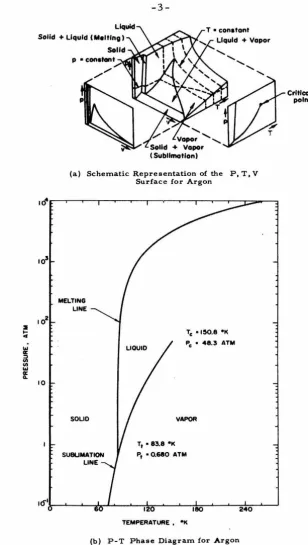
In this thesis we will develop molecular models of sublimation and melting (or freezing) for monatomic elements and apply these models to the rare gases. In Fig. 1 we have indicated the transition lines that we will study on the phase diagram of argon.

The thesis is divided into two parts. In Part I a simple mo-lecular model is used to represent sublimation of a solid. With this model the basic mechanism of the phase transition is easily seen.

The equilibrium vapor pressure is calculated and an estimate of the latent heat of the transition is made. The model is applied to argon, krypton, and xenon and excellent agreement with experiment is found.

10

-3-(a) Schematic Representation o{ the P, T, V Surface for Argon

MELTING

LINE

SOLID

LIQUID

T, • 83.8 91<

Tc •l~.8 •K Pc • 48.3 ATM

VAPOR

Pt • 0.680 ATM

180 240

TEMPERATURE , 91<

(b) P-T Phase Diagram for Argon Fig. I Phase Diagrams for Argon

[image:8.562.120.428.57.602.2]

-5-PART I

II. FORMULATION OF A MODEL OF SUBLIMATION

A. INTRODUCTION

In the past, studies of sublimation have been focused on the

determination of the vapor pressure of the solid. By noting that the

two physical systems, the gas state and the solid state, are in

equi-librium, a relation between the vapor pressure and the critical

tem-perature may be calculated(S,

6 ).

For a monatomic solid, the vapor pressure is given by the

expression (S)

.tnp dT'

kT12

(II- I )

where Lo is the heat of sublimation per molecule at 0°K, cp is

the heat capacity at constant pressure per molecule of the crystal,

m is the atomic mass, k is Boltzmann's constant, and h is

Planck 1 _{s constant divided by 2iT.}

Empirically, the vapor pressure may be related to the

tern-perature by a relation of the form

1

1n p = -

z

1n T

-L +E 0 0

kT (II-2)

where E is the lattice zero-point energy per molecule and w is

0 g

the "geometric mean frequency" of the lattice vibrational spectrum.

Salter(6) has derived Eq. (II-2) from first principles assuming

-7-ideal vapor for T ? (JD/2, where (JD is the Debye temperature. The calculations of the vapor pressure of solids as exempli-fied by Eqs. (II-1) and (II-2) do not shed much light on the nature of the phase transition. In those analyses, the solid and gaseous states

are treated as if they were different physical systems rather than two phases of a single element.

It is the purpose of this Chapter to develop the theory of sub-limation in a new manner by considering sublimation as a bridge be

-tween the solid and the gas states. The solid and gas phases arise as two components of a single particle system. A critical

tempera-ture, Tc' can be defined such that at temperatures less than Tc' the system behaves like a solid; and for temperatures greater than T ,

c it is a gas. As the temperature increases across T , c we find that a latent heat, L, will accompany the phase transition; and L is related to T . Moreover, the variation of the vapor pressure

c

with temperature can be calculated. It is found that the vapor pres -sure is related to the environment of the particle in the gas state.

B. THEORY

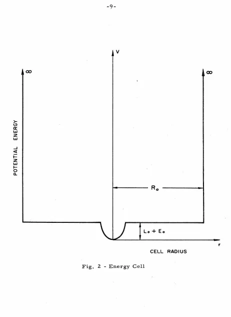
To represent sublimation, we assume that the solid-gas system can be represented by N independent particles, each in its own cell. The potential, which characterizes the cell, is assumed to represent the aggregate interaction with all other atoms. When the energy of the particle is lower than a certain energy, E

E~ E

l (II-3)

where w is the Einstein frequency(?) and r is the excursion from

the equilibrium position.

At E • the particle suddenly experiences a free particle l

potential

V=E

l

E>E

l (II-4)

Each particle is confined to a cell which is shown

schematical-ly in Fig. 2.

For energies below E • the particle energy states(S) are l

with degeneracy

e = hw(n+3/ 2) n

(n+l )(n+Z} g _n

=

(II-5)

(II-6)

For simplicity, we neglect the interaction of the free particle

with the harmonic potential when the energy of the particle is greater

than E,. This is justifiable since R₀

»[m~'

Ji

for all cases under

consideration.

We will find that the free particle states are essentially

con-tinuous; therefore, we can express the density of energy states (the

>-Cl

a::

w 2 w

,oo

-9-v

) lo+ Eo

CELL RADIUS

Fig. 2 - Energy Cell

00

[image:14.559.54.516.47.680.2]

D(e -E )

l

1

= (2m3)2 V c (e -E

)~

2irz h3 l

(II- 7)

where V is the volume of the cell containing the free particles. c

This density of energy states is independent of the shape of V . We

c

expect V to decrease with increasing pressure. The idea that

c

dense gas particles should be considered as confined to a volume much less than the total volume of the container was proposed by

( 1 0) Lennard-Jones and Devonshire .

At low temperatures, we expect the energies of most particles to be less than E , thus we have essentially the Einstein model(?)

l

which is in good agreement with experiment for temperatures above

bw/k for a solid. At high temperatures, we have an ideal gas.

The partition function, Zt' for the system is

Z - ZN

t

-where Z is the partition function for a single particle.

exp(-e /kT)g

n n

alle n

. where e denotes a single particle energy state. n

For our model we have M

(II-8)

(II-9)

z

=

l

n

(n+l )(n+2)

2 exp (-( n+ i}hw/kT

)+

SEoo

D(e -E1 )exp(-e /kT)de l

(II-10)

11

-(II-11)

We have used the discrete energy spectrum in Eq. (II-1 O) be-cause quantum effects of the harmonic oscillators are present near

the triple point of rare gas solids. This has been noted by

Moelwyn-Hughes (l l

>.

If the ratio of kT and hw is large, we can use a con-tinuous approximation for the density of states of the solid. This approximation is treated in Appendix A.

Let us denote

L

0

=

E₁ - } hw (II-12)

which can be interpreted as the zero-point latent heat. Also, it is convenient to define the new variables:

and

x =

exp ( -

nw

I

k T)

v

_c

A=

n=o

= aV

s

41T3/z (nw )3/z

C =kT/hw

(II-13)

(II-14)

(II-15)

(II-16)

(II-1 7)

where V is the average atomic volume in the solid, which is es -s

With the use of Eqs. (II-7) and (II-11) - (II-17), then Eq.

(Il-1 O) becomes

Z =

x

3

/z[

~·

+ 2XI' +I+ aA exp(-L

0 /kT)C 3

h]. (II-18)

where I' and I" are respectively the first and the second derivatives

of I with respect to X.

The free energy and the internal energy are given by

F

= -

kT log zt (II-19)

and

o(F IT) v

8T

(II-20)

By using Eqs. (II-8), (II-18), (II-19), and (II-20), we find the

energy

=

~

I"'+

µ.

X' I"+ 6XI' +

~

I+aA exp(-L

0/kT)c>'z

[~

+(C+l

lf]

xz.

3/

2

I"+2XI'+I+aAexp(-L

0 /kT)C 2

(II-21)

where I"' is the third derivative of I with respect to X. We note

that

is a,

I

=

1-XM+l

1-X (II-22)

It is clear that the only undetermined parameter of the model the number of volumes V available to the free particle,

s We

also noted that V decreases with increasing pressure. Let us then c

take

-13-where a(p) decreases with increasing pressure.

It is instructive to examine Eq. (II-21) in detail. We note

that

E

=

E(T, w, L

0 , .Aa(p) ) (II-24)

For low temperatures, the energy is that of a collection of harmonic

oscillators and for high temperatures, we have the energy of an ideal

gas. In fact, for either temperature extreme, the energy is inde -pendent of a(p). In the application of this model to argon, krypton, and

xenon, we will demonstrate that a(p) is only important near the

transition point, T , defined by c

(II-25)

where C is the specific heat at constant volume. For this reason, v

we define the pres sure of Eq. (II-23) to be the equilibrium vapor

pressure. From Eqs. (II-24) and (II-25), we have

T

=

T (w,L ,Aa(p))

c c 0 (II-26)

For a particular solid, Eq. (II-26) becomes

T

=

T (a(p) )

c c (II-27)

Equation (II-27) yields the equilibrium vapor pressure curve, once a(p) is known.

For most practical applications, T is essentially independ-c

(II-28)

This is exactly true for the clas.sical solid described in Appendix A

if A is replaced by A .

l

Therefore, for solids with similar molecular structure, such

as the rare gas solids, one might expect from the law of correspond

-ing states (Ref. 12,p. 19J that for some characteristic pressure

(II-29)

In Table I, we illustrate the experimental relationship of Tc and L 0

for argon, krypton, and xenon at their triple point temperatures, Tf

TABLE I

Ratio of zero-point latent heat and kT t

Element L0 /kT;

Argon 11. 08

Krypton 11. 58

Xenon 11. 93

:!,c

Calculated from values given by G. L. Pollack, Rev. Mod. Phys.

TABLE II Physical Constants Zero-point Zero-point Atomic Average latent heat energy mass atomic volume Triple Point e E (cal/mole)e

v

(A

3 ) Element L (cal/mol) m(amu.) Pt(mm~ Tt(OK) 0 0 s Argon 1846a 184,6b 39.948c 39. 73d 516,86a 83.810a Krypton 2666a 145a 83,80c 45.19d 548, 7a 115. 78a Xenon 3828a 123a 131.30c 59.62d 612,2a 161.37a

a G.

L. Pollack, Rev. Mod, Phys. 36, 748 (1964). bPollack gives 187 cal/mole and G.G. Chell and I, J. Zucker, J. Phys. C(Proc. Phys. Soc,), Ser. 2 . ,

_!,

35 (1968), give 182, 3 cal/mole. We use 184 , 6 cal/mole for numerical convenience. cR. C. Weast, Handbook of Chemistry and Physics (The Chemical Rubber Co., Cleveland, Ohio, 1967-1968)48thed. p. B3. dCalculated from nearest neighbor distances given by Pollack. ewe convert these values to energy per molecule for this analysis.

c.

APPLICATION TO ARGON, KRYPTON, AND XENON

1. Preliminary Calculations

To apply the theory, we need to calculate E(T) given by Eq.

(II-21) and its derivatives. To calculate the constants of Eq. (II-21) we need the following physical constants: the zero-point latent heat,

L

0 , the zero-point energy, E , 0 the atomic mass, m, and the average atomic volume in the solid state, Vs. Vle will also need

the triple point pressure, Pt' and the triple point temperature, Tt' for future reference. These constants are given in Table II.

The zero-point energy is given by

3

E₀ =

z

hw (II-30)

By using the physical constants of Table II and Eqs. (II-11) and (II-16),

we may calculate M and A for each element. These constants are

listed in Table III.

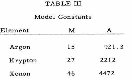
TABLE III

Model Constants

Element M A

Argon 15 921.3

Krypton 27 2212

Xenon

46

4472

The energy may now be calculated from Eq. (II21) as a func

-tion of temperature with the parameter a. The internal energies of

argon, krypton, and xenon are shown graphically in Figs. 3, 4, and 5

respectively, for selected values of a. The phase transition is

[image:21.559.170.396.393.529.2]

2

.

0

0

...J 2

'

UJ

.

~

/

11.0~

I

I

/

I

I~

...J

<t

'

2

I

a:

UJ

2.0

0 _{_J}

z

_...

w

.

>-

_~

a:

w

1.0

z

w

_J <X

z

er:

w

I-

z

0

0.1

0

.

2

0.3

0.4

0.5

TEMPERATURE,

kT/Lo

Fig.

4

-Internal

Energy

of

Krypton

a

Tc

500

107.1

°K

20,000

82.4

°K

0

.

6

0.7

0

.

8

2.0

0

_J

z

'

UJ

.

>-

(!)

a:

UJ

1.0

z

UJ _J <l

z

a:

UJ I- 2

0

0.1

0.2

0.3

0.4

0

.

5

TEMPERATURE,

kT/Lo

Fig.

5

-Internal

Energy

of

Xenon

a

2,000

2,000,000

0.6

Tc

136.0

°K

90.4

°K

0.7

I _{... ..!:)} I

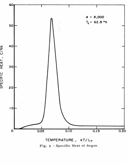
The specific heat,

Cv=(:~J

(II-31)

v

may also be calculated from Eq. (II-21) by differentiation. The shape

of the specific curve is shown in Figs. 6, 7, and 8 for argon, krypton,

and xenon, respectively. The critical temperature of each curve is

about 75 percent of the triple point temperature. We note that krypton

and xenon are behaving as nearly classical solids before the

transi-tion temperature is reached, but that argon is not.

2. Identification of the Equilibrium Vapor Pres sure

To this point, we have been using a as a free parameter.

As we vary a, we change the critical temperature. This is shown

in Figs. 3, 4, and 5, This behavior was predicted by Eq. (II-27). As

we noted in the previous section, if we know the functional form of

a(p) we can determine the vapor pres sure curve from Eq. (II-27 ).

With the knowledge that a(p) is a decreasing function with pressure

and that a(p) is proportional to the volume seen by the free particle,

we assume

Q

=

G

p (II-32)

where G is a constant and p is the equilibrium vapor pressure.

Since our model has no provision for a third phase, the liquid state,

we shall adjust G to the triple point data. We list in Table IV the

values of G found for the elements studied. By numerically

differ-entiating Eq. (II-21 ), we may calculate the critical curve by using

50

.le: 40

[image:26.562.80.499.121.666.2]

z

...

u

t-c:i

w

30

I

u

LL.

u

w

CL

(f) ₂₀

10

0 0.05

-21-0.10

a •

e,ooo

Tc• 62.9•K

0.15

TEMPERATURE , kT

I

Lo

Fig. 6 - Specific Heat of Argon

50

.:itt:. 40

[image:27.562.50.502.102.660.2]

z

...

u

-...

<X

UJ

30

:I:

u

LL

u

UJ

CL

Cf) ₂₀

10

0 0.05

a

"'

8,000 Tc• 87.4 °K

0.15

TEMPERATURE, kT I Lo

Fig. 7 - Specific Heat of Krypton

50

~ 40

[image:28.562.51.493.84.617.2]

z

...

u

1--<I w

30

I

u

u..

u

w

a.

U) 20

10

0 0.05

-23-0.10

a

= 10,000

Tc• 121. 7 •K

0.15

TEMPERATURE 1 kT /Lo

Fig. 8 - Specific Heat of Xenon

TABLE IV

Product of a-p

=

G

Element G(mm X 105)

Argon

1.

00

Krypton

1.

08

Xenon 1. 42

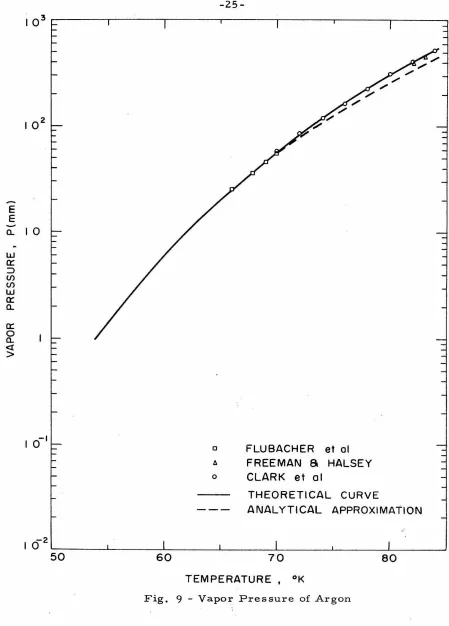
experimental data in Fig. 9 obtained by Flubacher, et al(l3)•.

(14) (15) .

Freeman and Halsey , and Clark, et al for argon. In Fig. 10

we compare the vapor pressure of krypton measured by Beaumont,

(16) . (17) (14)

et al , Fisher and McMillan , and Freeman and Halsey

with our theoretical curve. Finally, we compare our results with

( 14) the vapor pressure of xenon measured by Freeman and Halsey ,

Podgurski and Davis(lB>, and Peters and Weil(l 9 ) in Fig. 11. We

note that Freeman and Halsey(I4) gave an experimental curve; the

figures show selected points of these curves. We conclude that our

assumed relation (II-32) is valid.

Although a theoretical interpretation of G has not been

found, we mention that G is the same order of magnitude as

atkT/Vt, where atV s is the volume of the free particle cell and

Vt is the volume per particle of an ideal gas at the triple point. We

can see from (II-32) that G would be exactly this value if the vapor

could be considered an ideal gas and the aggregate interactions were

negligible. We may state this interpretation more clearly by noting

[image:29.562.62.477.60.445.2]

I 02

E

E

a_ ₁₀

UJ

Q:: ::> CJ) CJ)

UJ

Q:: a_

Q::

0

a_

<[

>

60

0

A

0

-25-FLUBACHER et al FREEMAN 8 HALSEY CLARK et al

THEORETICAL CURVE

ANALYTICAL APPROXIMATION

70

TEMPERATURE , °K

80

[image:30.559.44.493.54.680.2]

E

<l::

, 10

w

ex:

.:::> (/) (/)

w

ex:

a..

ex:

0 a.. <X

>

60

o BEAUMONT et a I

0 FISHER

a

McMILLAN

A FREEMAN 8 HALSEY

THEORETICAL CURVE

70

80

90

100 110 120 TEMPERATURE.' °K [image:31.563.37.497.47.649.2]

-27-o FREEMAN 8 HALSEY

o PODGURSKI 8 DAVIS

t. PETERS

a

WEIL

. THEORETICAL CURVE

E E

-

a..

10

IJ.J

a:

::>

(,/) (,/) IJ.J

a:

CL

a:

0

a. <[

>

TEMPERATURE ' °K

[image:32.562.12.515.36.678.2]

By taking values of a smaller than the triple point value, we

begin to trace out the condensation curve of Fig. 1. We can see from

Fig. I that the sublimation line and the condensation 1 _{ine join very}

smoothly. This is as we would expect since these transitions are

physically similar as long as the liquid density is near solid densities.

Analytically setting the second derivative of E with respect

to T equal to zero is very tedious. In Appendix 3 we calculate an

approximate expression for the vapor pressure a~1alytically. We

find

L

1 n p =-k

~

- } 1 n C

+

1n[C2 {I - e - I / C ) 3)

+

1 n [I +f (

~w

, T)]

+

1 n [ GA) ,,(II - 3 3 ) 0

where f

(~

, T ) - 0 as ti.w -+ O. In deriving Eq. {II-33), we have

o Lo

assumed

and

L 0 ti.w

»

I

(II-34)

(II-35)

We can not neglect f

(t: ,

T)

in Eq. {II-33) since it is as

large as 0. 6. For. argon, we find

=

hw

[.!.,l

C _

65

cz _

9X

+

81 XC _

s

21 X 2

J

+o[(hw)

2

J.

L ₀ 2

8

I - X

Z

I - X (I _ X )2 L z

0

(II-36)

[image:33.564.36.499.150.622.2]

-29-of argon is shown as the dashed line in Fig. 9 . . Since Eq. (II-33) is

already more cumbersome than Eq. (II-2) no further approximations

were attempted.

In concluding our study of the equilibrium vapor pressure, we

demonstrate one of the advantages of this model. As we noted,

pre-vious studies have considered sublimation as the equilibrium of two

physical systems. We can do this by considering the solid and gas

phases to be in equilibrium. For the partition function of the solid,

we have from Eq. (II-18 ),

Zs

=

x

3/2 [

X?"

+

2XI'

+

1] (II-37) and for the gas_,

-L /kT

z

= etAe o Cl/Z Xl/Z

g (II-38)

By equating the chemical potentials of these separate systems and

using Eq. (II-32) we find the vapor pressure is described exactly by

Eq. (II-33) with

f(~:

, T) equal to zero. This leads to a large error

in· p. With this approach we have lost the inherent corrections due

to vacancy formations of our cell model. These corrections must be

handled separately as Salter demonstrates.

3. Estimate of the Latent Heat

Finally, we want to calculate the latent heat. Since the energy

is a continuous function of T, the beginning and end of the transition

is not precisely defined. Therefore, the latent heat is somewhat

L = AE

+

pAv

We have found that (for a

»

I),

pAv = pa V

s

By using Eq. (II-32 ), we have

pAv

=

GVs

(II-39)

(II-4 0)

(II-41)

Figures 3, 4, and 5 indicate that ~E is the order of L for all T .

0 c

We choose to define AE by extending the "natural" tangents of the

energy curve above and below T as shown in Fig. 12. We are in

. C .

part assuming that the specific heat at constant pressure and C v

are nearly the same. With this definition of AE, we find by similar

triangles

(II-42)

where

Nk(

cv) is the average specific heat at the point of inflection

of the specific heat curve of the solid as sublimation begins and J is

the intercept of this tangent line.

Therefore, as an approximate expression for the latent heat,

we have

(II-43)

For argon, krypton, and xenon, we find ( cv) to be 2. 50, 2. 75, and

2. 95, respectively, and J to be . 046, . 018, and. 005, respectively.

[image:35.560.51.498.50.468.2]

0

....J

z

...

w

.

>-

~

a:

w

z

w

....J <(

z

a:

w

t-

z

I+

Eo Lo

6E

/

Lo /

/

/

/

/

/

I

/

/

vV

I

/

/

////

/

/

/

/

//

/

/

/

Eo I Lot.;-'

1

J

kTc/L

0

TEMPERATURE,

kT/Lo

Fig. 12 -Method of defining the change of internal energy for sublimation. With this definition of

aE,

L =

aE

+

GV S '

since the corrections resulting from its dependence on T are small c

and these corrections are less than the inherent uncertainty of

Eq. (II-43 ). We note that an error in the estimate of ( Cv) is

com-pensated for when J is calculated. For a variation of ± . 02 in

<

Cv>• we find L varies less than 1/2%.

With this definition of L, we compare the theoretically

estimated values with the experimental data at the triple point in

Table V.

TABLE V

Latent heats at the triple point

Element

Argon

Krypton

Xenon

>!:::

G. L. Pollack, Rev. Mod.

Theoretical

(L/ L

0 )

1. 01

0.963

0.948

Phys. ~. 748 (1964).

D. CONCLUDING REMARKS ON SUBLIMATION

1. Summary of Results

Experimental

(L/ L )':c

0

1. 01

. 967

. 901

The agreement between the theoretical and experimental

results as shown in Figs. 9, 10, and 11, is indeed very remarkable.

At this point, it is especially noteworthy that, for each element, the

only unknown parameter is G, since L and E may be obtained

0 0

[image:37.562.67.468.90.551.2]

-33-curve, e.g. the triple point, then determines G unequivocally. In this connection, we may remark that Eq. (II-2), as derived by Salter, consists also of one parameter, w,

g which has to be deter -mined by experiment in practice. But the range of validity of Eq. (II-2) is somewhat less than the present theory. For example, Eq. (II-2) begins to deviate from experimental data for krypton at

about 75°K; but this rmdel is consistent with all experimental data available.

The sublimation process according to the present model does not represent a singularly sharp phase transition. Although, whether the transition is in fact a sharp transition is still not a settled question,

we do not intend to raise this issue here. We only point out that the energy and specific heat curves as shown in Figs. 3, 4, 5, 6, 7, and 8 clearly reveal a phase transition across the temperature region in

the neighborhood of T . In fact, the transition becomes sharper as c

T becomes smaller. c

The mechanism of the sublimation process can also be seen from this physical model. The tendency for the system to stay at a lower energy in the harmonic potential is constantly competing with

the tendency to be in the free particle cell at higher energy. The Boltzmann factor will favor the lower energy states. On the other

hand, the free particle cell provides a much larger number of

avail-able states. The sudden predominance of the large density of states for the free particle cell over the Boltzmann factor across a narrow temperature range results in the sublimation transition. This

we believe, underlies all the phenomena of phase transition. The system will change from one phase to another when the latter has a much larger density of states even at the expense of a finite jump in

energy. This jump in energy gives rise to the latent heat.

For the present physical model, sublimation is not a

discon-tinuous process. So there is some ambiguity in defining the latent heat. We have defined L as shown in Fig. 12. The inferences of such a definition are consistent with all experimental evidence. The

latent heat thus defined varies slightly with Tc. From the physical model, we can see that it tends to L

0 at 0° K. For the nearly classical solids in the temperature range where this theory is valid, L decreases as T increases.

c

We have represented the solid phase by the Einstein model <7) mainly because we are primarily interested in the problem of

sub-limation. In the temperature range in which we have been interested, the Einstein model gives nearly as good a representation as the De bye

model{2l ). The use of the Einstein model yields a simple picture of a particle confined in a cell, and enables us to visualize graphically

the process of sublimation. At low temperatures, we need to r evise our representation of the solid state to accommodate the inadequacy of the Einstein model. Also, we may need to incorporate the an-harmonic effects in our model to deal with the situation in the im-mediate vicinity of the triple point.

2. Suggestions for Further Research

-35-of study where the ideas developed here may be used or tested.

i) Formulation of a simple model may be instructive in isolating

the principles involved in any phase transition that one is studying.

For example, such a model of melting may be very useful in

improv-ing our understandimprov-ing of the liquid state.

ii) Experimental measurements of the specific heat, as the

sub-limation line is crossed, would determine how sharp the transition is.

This data along with measurements of the latent heat as a function of

sublimation temperature will determine to what extent our model may

PART II

37

-III. INTRODUCTION TO THE THEORY OF MELTING

A. REVIEW OF PREVIOUS WORK

A comprehensive review of the theory of melting is not

avail-able in the literature. Reviews of selected aspects of the theory have

been made by Ubbelohde (22) (for complicated molecular structures),

Cohen (2 ) (selected mathematical models). and Brout(l) (existence

and stability of the phases). Reviews of the melting

(23)

rare gases have been made by Dobbs and Jones •

theories of the

Pollack ( 24) • and

Horton (25). In the following paragraphs we will give a. brief review of

the existing theories of melting.

A successful theory of melting does not exist at the present

time, That is to say. there is no molecular model from which one

can demonstrate from first principles a transition from the solid

state to the liquid state or vice versa. This theory must predict the

melting curve and the changes in volume, _fl.

v '

m and entropy, fl.

s '

m

of melting. The main difficulty found in formulating such a

funda-mental model of melting is the lack of a good theoretical

representa-tion of the liquid state.

In the past, the study of melting has been concentrated in two

areas. The first area of research deals mainly with the

establish-ment of the existence of the transition. Examples of work in this

area includes the general study of phase transitions by Yang and

Lee(26) and the studies of melting by Kirkwood and Monroe<27) and

Brout(l). The second area is concerned with correlating the physical

our interest to the latter.

Since the molecular structure of argon is relatively simple for

theo;i:-etical calculations and a large reservoir of experimental data

is available, it has been customary to apply melting theories to argon.

In this thesis, we will follow this custom.

An essential feature of any phase transition is the existence of a critical temperature above which the transition does not exist.

For the melting transition the existence of a critical temperature is not

. (28) - (30)

a settled question . However, the general belief, based on the experimental results of Bridgman{3l) and Lahr and Eversole <3Z )'

is that no critical temperature exists.

1. The Lindemann and Simon Equations

The fir st molecular model used to explain the melting of a

solid was formulated by Lindemann<33) in 1910. He assumed that melting occurred when the thermal vibrations of the solid molecules became so large that the adjacent molecules could touch. The result-ing formula is

(v

)3/z.

m m

ez.

T

=

constant (III-1 )

m

where V is the volume and T is the temperature along the

melt-m m

ing line.

e

is a characteristic temperature (not necessarily the

De bye or Einstein temperature). Although we know that such large

amplitudes are not found, the success of the Lindemann equation in

predicting the form of the melting line for a large number of

-39-had only limited success<34) - <33

>.

Other than its pheno1nen0Jogical nature, the majqr weakness of the Lindemann model is its inability to give any prediction of the change in the entropy or volume as soci-ated with melting. Therefore, we do not have any estimate of the liquid properties adjacent to the melting line.

A more useful melting equation would relate the melting pres -P with T • Salter<39> has shown that the Lindemann

equa-m m

sure

tion may be combined with the Griineisen equation of state of a solid to give a melting equation in the form

(III-2)

where .J!.. and .£ are constants. This equation was originally proposed by Simon and Glatzel(40) from experimental observations and it is known as the Simon melting equation. Babb(4l) has listed the empirically determined values of i!.. and ..£.. for many

sub-stances. These constants for the rare gases are given in Table VI.

TABLE VI

The Simon Constants of the Rare Gases

>:C

Element

Argon Krypton Xenon

~'

a(bar s) c

2114 _1.593

2376 1. 617

2610 1.589

Neon and radon will not be considered

More recently, Gilvarry(37) and Babb(3B) have used tlwir

quanturn-mechanically corrected versions of the Lindemann formula

and the Murnaghan equation of state of a solid to derive the Simon equation in a manner similar to that of Salter. (We note that all of these models approach melting from the solid side of the melting curve.)

2. Order -Disorder Theories

One of the more successful theories of melting is the

order-disorder theory developed by Lennard-Jones and Devonshire (42 ), (43 )_

They assumed that the melting system is composed of two interpene -trating lattices. When the system is in the solid state essentially all molecules are on one lattice structure. After melting, the molecules are nearly randomly distributed on the two lattices (short range

order may exist after melting). The formulation is based on the theories of binary alloys of Bragg and Williams (44 ), (45) and Bethe(46).

This model is the Ising model(47),and it has been widely

studied(

4

B~

(49).

Although the interpenetrating lattice structure is not a physical

reality, the qualitative agreement with experiment at low

tempera-tures is good. In Table VII the results of this order-disorder model

are compared with experiment, for selected points near the triple

41

-TABLE VII

Melting Properties of Argon

>:<

Derived from the Lennard-Jones and Devonshire Model

Physical Quantity ~ m V/V ~ m S/k P /dyne -c:-m :n

~(~)/°K

(83. 8°K. (90. 3°K) (Liquid)

Method of Bragg and I. 35 1.70 286X 106 0.0040 Williams

Method of Bethe 1.28 1. 74 294X 106 0.0049

'

Experimental

o.

12 1.60 291X 106 0.0045

>:<

J. A. Barker Lattice Theories of the Liquid State (Pergamon Press, Oxford, 1963), p. 41.

This apparent success of the order-disorder model is of

limited value since it has a critical temperature. For argon, this

critical temperature is near 130° K; however, the melting transition

has been observed up to 360° K and, as we indicated earlier, there is

no indication of a critical temperature. A second weakness of the

order-disorder model is found when more accurate mathematical

representations are used; it is found that the agreement between

theory and experiment becomes poorer. This behavior indicates that

many of the physical features have been hidden by the semiempirical

selection of the model parameters in the less accurate representation.

We conclude, as other have, that there is a fundamental difference

between melting and the order-disorder transition and that further

[image:46.559.66.485.159.291.2]

3. Hard Sphere Models

In recent years, some promising developments in the theory

of melting have been made by assuming that the major contribution to

melting comes from the hard core part of the intermolecular poten-tial. The molecular dynamics calculations by Alder and

Wainwright(50) - (52) and Alder, Hoover, and Wainwright(53) of hard spheres and disks have demonstrated that a phase transition exists for this simple interaction. A typical isotherm is shown in Fig. 13.

PV

P.r

V/V

0

Fig. 13 Phase Transition of Hard Spheres

More recently, Longuet-Higgins and Widom (54) have

ap-proximated the melting system by hard spheres plus an average

contribution resulting from attractive forces. The average attractive

potential is

2a cJ> ATT.

=

-

V

And the resulting equation of state is

P = P - a/Vz H.S.

(III-3)

(III-4)

[image:47.560.66.487.75.666.2]

-43-By a suitable choice of _a_ , they found excellent agreement with experiment at the triple point. Sarne of their results are shown in

Table VIII.

TABLE VIII

Melting Properties of Argon

Derived from the Longuet-Higgins and Widom Model

>'<

1 n(PV₁ /kT )~ (aS/k)~

'"

>'< (E₁ /kT )~

::::::

Theory 1. 19

Experiment 1. 114

-5.9

-5.88

1. 64

I. 69

-8.6

-8.53

The subscripts 11_{£ ",} 11_s11_{, and "t" will refer to liquid, solid, and} triple point respectively throughout the remainder of the text. E is the internal energy.

The agreement between theory and experiment is impressive;

however, for higher temperatures the theoretical predictions become

very poor. Crawford and Daniels <55) have shown that this model may

be corrected to account for this high temperature region by using (III-3) and (III-4) for the liquid and by calculating attractive potential

in Eq. (III-3) from a Lennard-Jones potential for the solid. This

assumption gives rise to a new parameter Vb' For molecular

volumes above Vb the liquid equation of state is used and for

volumes less than Vb the solid equation of state is used. The

result-ing model has two parameters vb and a that are determined by

semiempirical means.

Finally, the most elegant analysis of the melting problem,

Barker (Sb). By using their recently developed hard sphere

perturba-tion theory of liquids and the Lennard-Jones and Devonshire (l O) cell

model for the solid, they have calculated the melting curve of argon,

Fig. 14. The melting pressure is obtained from the slope of the

common tangent in a plot of solid and liquid free energies versus

volume. The change in volume and entropy of melting have not been

calculated with this model.

-

E

g

[image:49.560.101.425.255.446.2]

P-t 0

...

b.O

0

~ 4

3

0

o Experiment

Theory of Henderson and Barker

100 200 T(OK)300 400

Fig. 14 Melting Line of Argon

The success of these models has lead to a general belief that

hard sphere packing is the essential feature of melting.

4. Other Models

We will not attempt to list all other models; however, we

would like to note two interesting approximations. Emtage <57) has

assumed that the essential feature of melting is the mismatch of bits

of lattice structures as the solid melts. The resulting melting curve

-45-with experiment.

In the second model by Tsuzuki(5B), the two body distribution

function 41Tz g(r) is assumed to be constant for r. ( l -~) ~ r ~ r. ( l +~),

1 1

where r. is the location of the ith shell of neig1_{1boring molecules}

1

in the solid, and ~ is a measure of the liquid irregularity. A free

volume approximation is used for the entropy. With this crude model,

the change in volume, the change in entropy, and the melting

tempera-ture are calculated for the case P :::: 0 (the triple point). The m

calculated melting temperature is 0. 82 in reduced units compared to

the experimental value, 0. 67.

5. Summary of Existing Theories

In the preceding paragraphs, we have tried to give a complete

picture of the current state of the theory of melting. We would like

to point out that none of these theories predicts from first principles

the melting curve, the change in volume, and the change in entropy.

(The model by Henderson and Barker is most closely aligned with

fundamental reasoning.) We have also indicated that many models

have been developed with semiempirical parameters. It is suggested

that these parameters may be concealing important physical

phenom-ena. We believe that this review has demonstrated the need for a

melting model, developed from first principles, from which a

B. PURPOSE OF THIS STUDY

We will develop a theory of melting from the fundamental point of view. By assuming microscopic models for the solid and

liquid states, the macroscopic properties are computed with statis

-cal mechanics. The melting points are then determined in a formal way by equating the chemical potentials of the solid and liquid states. The validity of the solid and liquid models near the melting curve will be studied. The models selected were believed to be the best available at the outset of this study.

We have made only four assumptions in formulating this melt-ing model.

1) The configurational energy of any collection of atoms is the sum of the energy of pairs of atoms.

2) This configurational energy for two atoms a distance r

( 3) .

apart may be represented by the Lennard-Jones ( L.T) 12 -6 potential. The LJ potential is

The pair potential is regarded as

a

basic physical quantity. Ideally

the constants for u(r) would be determined from a

quantum-mechan-ical calculation of the force between two atoms<59). However, in practice these constants are determined from experimental measure-ments of the second virial coefficient of the gas(60). For argon, we have

-47-and

a=3.4os.A

(III-7)

Although Eq. (III-5) with the consta.nts defined above is generally

accepted as the "best" pair potential function for argon, considerable

effort is being made at the present time to determine u(r )(6l). Since

there is some uncertainty in u{r). we will discuss the effect of slight

shifts in E and a.

3) We will represent the solid by an anharmonic model

de-( 62) . (63)

veloped by Henkel and Guggenheim and McGlashan . The

anharmonic effects are calculated from a perturbation theory of a

harmonic oscillator. The oscillator frequency and the perturbation

energy are computed directly from lattice sums of the pair potential

function, Eq. (III-5 ). This solid model is compared with the widely

used cell model of Lennard-Jones and Devonshire(l 0

>.

4) Finally, we assume that the Percus-Yevick (PY) equation

is a valid approximation for the liquid state. Recently, Watts<64\(65)

has shown that the thermodynamic functions predicted by the PY

ap-proximation are in excellent agreement with experiment for moderate

liquid densities. Details of this assumption will be discussed in

Chapter IV.

Although the validity of the first three assumptions may be

questioned, th~y are generally used in the study of the rare gases.

There has been considerable controversy, however, concerning the

merits of the PY equation. Therefore, a basic aim of this study is

we have assumed I) - 4),the properties of the systerr1 are determined.

The liquid state properties will be studied along three iso-therms (kT/E == 1.3, 1.8, and 2.0) above the liquid-vapor critical

point. These isothcrnH> are 8hown schernaticaUy on the pha8e <lia-gram in Fig. 15.

Temperature Fig. 15 Schematic Diagram of the

Isotherms Studied.

[image:53.559.69.486.93.390.2]

-49-IV. THEORY OF MELTING

A. THERMODYNAMIC CONDITIONS FOR MELTING

We may represent the equilibrium of the solid and liquid phases by equating their chemical potentials

(lV-lJ

Once we have an equation of state for each phase and Eq. (IV-1) is satisified, we may immediately calculate the volume change and the latent heat of the transition.

For the solid, we have

µ. _s = F _s.

+

PV _s (IV-2)

where F and V are the free energy and the volume per particle

:i::::

respectively . These thermodynamic quantities will be calculated in

a later section.

Similarly for the liquid, we have

(IV-3)

We calculate the pres sure by using the relation

P=

- av

oF)

_T (IV-4)

We differentiate Eq. (IV-3) with respect to volume. By using Eq.

>::::

(IV-4), we fin<l

(IV-5)

Integration of this relation along an isotherm from state (1) to state

(2) gives

(IV-6)

By adding and subtracting the same quantity, we have

(IV - 7)

We rewrite this in the form

µ1 (2)

kT

-s2

[VJ. 1

J

µ1(1)

- l _{kT - pl dP1 +1nP(2)+ kT -.lnP(l)} .(IV-8)

T=constant

By letting P(l)-+ 0, state (1)-+ ideal gas; for an ideal monatomic gas (Ref. 12, p. 15), we have

(IV-9)

By using this relation in Eq. (IV-8 )~ we have

µ~~)

=

s

P(2)[l _ p1kTJ dP1 +ln [(Z-rr 3/Z h3P(Z)J

-51-where

(IV-11)

Therefore, we may calculate the chemical potential at P(2) if we

have an equation of state of the liquid along the isotherm for all

pressures less than P(2 ).

B. THE LIQUID STATE

We shall not make an extensive review of the theories of

liquids. For such a review the reader may consult one of the many

b oo s k in . th fe ie " ld(l2), (60), (66) - (68) • We shall merely outline the

~:c

steps leading to our representation of the liquid.

For a liquid of N molecules, the Hamiltonian may be

writ-ten as

(IV-12)

where p. is the momentum of particle i, m is again the mass of a

1

molecule, and U(r

1

, • • • , rN) is the potential energy of the N

molecules located at r

1

, • • • , rN respectively. If we denote

p~n)(~,

. , r N)dr

1

• • • drN a.s the probability of finding a mole -cule in dr

1 at r , l another in dr at r z z , . . . , and another in

dr at r n'

n regardless of where the remaining N-n molecules are

:l,c

located, then we may write

N!

S S

-13

U(r , . . . rN) _

. . . Ve 1 dr n+ 1 • • • dr N

(N-n)!

ZN

where

13

is 1 /kT, V is the total volume (NV

1 ), and

ZN

=

s ... s

e

-13

U(r1 •

v

(IV-13)

(IV-14)

The function

p~n)

is known as the generic probability density.

We introduce the fugacity,

z

=

eµ/kT

In the grand canonical ensemble, we have 00

l

N ( ) - - 3N

z Z p n (r , . . . rn)/ (N~ A )

NN i

(n) - N :.>n

p (r , . .. r )

=

-1 n oo

l

1

(IV-15)

(IV-16)

where A is h(21TmkT)-2. A is called the thermal wave length of

the molecule.

We now assume that U is equal to the sum of potentials,

between pairs of molecules. This is the fir st assumption

U(r ,

l

...

'

-53-l~i<j~N

;

.

1)

J (IV-17)

By usin~ this assumption and Eq. (IV-16), we find upon differentiation of Eq. (IV-16) with respect to the coordinates of the molecule at r

l

(IV-18)

From (IV-18), we see that we have a hierarchy of equations in which (n) · d f" d · t f (n+ i) F th d ·

p 1s e 1ne 1n erms o p • or a ermo ynarn1c system, we have on the order of 1oz3 equations so that an exa~t solution is impossible. Therefore, one of the current problems in the theory of liquids is the determination of a successful method of truncating this hierarchy of equations. We shall find that the thermodynamic proper -ties may be determined if we know p <2). For this reason, the most effir::ient way to truncate (IV -18) is to make an approximation for p(3) in the equation for n

=

2. In the following paragraphs, we shall set up the analytic formalism necessary to understand our method of truncating (IV-18 ).

Since the liquid is in thermal equilibrium and it is macro-scopically isotropic, we may write

(2) - ~

p (r , r ) =

l z (IV-19)

(IV-20)

where

r=l;_;I

1 2 (IV-21)

The function g(r) is proportional to the probability of finding a mole-cule at a distance r if there is one at the origin; it is normalized to I for large r. The first equation of (IV-18) may be written with g(r) to give

- kT

~

g(r)

=

~

u{r)g(r)

+{v_Nl

2

S

~

u(

I; _; I

)p (3

>(; , ; . ;

)d;

1 1 y l 1 3 1 Z 3 3

(IV-22)

The probability of a third molecule being in dr at r when two

3 3

molecules are at r and r may be written as

1 z

and we find that Eq. (IV-22) may be expressed in the form

{ u(r)} I

s

-'1 1ng(r)

+

kT

= -

kT 'Vu(jr -r !)P(r Ir, r )dr

1 y l 1 3 3 1 Z 3

By rewritting this equation, we have

a

f

u(r)} 1

s

Brllng(r)

+

kT

= -

kT V

r•(r -r)

1 3

(IV-23)

(IV-24)

-55-This equation may be written in the form

(

u( r )+ W (r)

g(r) ::. exp - kT (IV-26)

where

(IV-27)

Therefore, a truncation of the heirarchy of equations, (IV-18),

may be made by making an approximation of W(r ).

Fir st we introduce a new function, c(r), called the direct

correlation function. c(r) is defined by the integral equation (Ref. 67,

p. 56)

N

s -

~

-g ( r ) - 1

=

c ( r )

+

V c (

I

r -r 1

I

) (

g ( r 1

) -1 )d r 1

.

v

(IV -28)

The advantage of introducing c(r) is that it is short-ranged in

comparison with g(r ). For large r, c(r) approaches O. By using

this fact, Baxter (

69 )

hao shown that if

c( r)

=

0

,

. for r > R (IV -29)

and if the integral of (g(r) -

1)

over all space is absolutely convergent,

then Eq. (IV-28) may be written as

g{r)-1 = c{r)

+

21T N

Sr

ds

S

s t{g(t)-l)(t-s)(g(t-s)- l)dt

r V o o

41T N

s

R

[S

s

s

j

r-s

I

]

+

r V sc{s) t(g(t)-l)dt- t(g(t)-l)dtds

0 0 0

+

4;

2

~:

S

0

R s c(s>[

S

0

for 0

<

r

<

R, where W(s, t) is defined by

W{s,t) = - W(t,s) (IV- 31)

and for s

>

t,

S

s [Ss-lt-ul

J

W(s, t)

=

u(g(u)-1) v(g(v)- l)dv du

o ls-t-ul

(IV -32)

Of course the integral condition is satisfied for any disordered liquid. With this form of Eq. (IV-28), the range of integration has been

reduced from infinity to a finite value, R, which in practice is only a few times the parameter cr. Therefore, Eq. (IV- 30) is very useful for numerical calculations.

As we have stated, we are interested in truncating the series of equations, (IV-18). We also indicated that this is most efficiently

...

done by approximating P(r Ir , r ) ~ which may be interpreted as an 3" 1 z

approximation of W(r) or vice versa. Recent calculations<64), <65) indicate that the most promising approximation for dense systems is the Percus-Yevick(4)(PY) approximation, which may be written as

~~)

= -

ln{g(r) - c{r)} (IV-33)

This equation is found by an elegant formulation of the many body

system in collective coordinates. Such a formulation lends itself to a

dense system; however, it was found that the PY equation would pre-diet the first four virial coefficients of the gas state. The implications of the PY equation have never been completely understood. The

57

-cluster expansion for c(r)

c(r)

=

[o-o]

+

~[~]+ ~

(IV - 34)

with the expansion consistent with the PY equation

c(r)

=

(o-o]

+

~[.6,]

+

~ ~z

[z

D +

4

0]+

, (IV-3·5)

where

-u(

1; _;

i)/kT

o - o = f =e 1 z -1

1 z

and

L S

= f f f dr V 1 Z 3 1 Z 3 3 1 z

, etc.

The PY approximation has neglected two classes of cluster integrals

for the higher orders of the density expansion; it is believed that

these integrals must essentially cancel each other.

Surprisingly, this equation has had little application at the high

densities for which it was derived(70). Therefore, an excellent test

of this equation can be made for the densities along the melting line. By combining Eq. (IV-26) and Eq. (IV-33), we have the PY equation

c(r) - g(r) (1-eu(r)/kT) _{(IV - 36)}

We have outlined a procedure for calculating g{r) and c{r)

from u{r). In order to determine µ

1 from Eq. {IV -10), we must

compute an equation of state. We may use the compressibility

equa-ti on

1

kT {IV-37)

and then integrate over the density to compute the pressure. For an

alternate method of calculating the pressure, we could use the virial

equation

pl. 21Tp 2

s

00

..e 3 du(r) ( )d

f f

=

P J. -

5KT"

r

err-

g r r

0

(IV - 38)

We will use Eq. {IV-37) since the rapid variation of du/dr and g(r)

· near r

=

cr is very significant in determining how accurately the

pres-sure may be calculated from Eq. {IV-38) with approximate

express-ions of g(r) and u(r). For the energy of the liquid, we have

3

s

00

E 1 =

2

kT

+

2 1T p J. u(r)g(r)r2dr

0 '

(IV - 39)

We have introduced these equations without proof. Again we refer

the reader to Rice and Gray(66) for a more detailed analysis.

C. THE SOLID STATE

As we have indicated in the introduction, we shall develop the

theory of melting from first principles. We assume that the two-body

interaction energy, Eq. (III-5), is a fundamental property of the

-59-require the crystals of the rare gases to be in a face-centered cubic

. (79), (80)

or a hexagonal close packed lattice structure . Although the zero

point energy of these two structures differ by only 0. 01%, the rare

gases are known to be in the face-centered cubic form for tempera-.

tures as low as 4. 2 °K(24). We assume that the solid is in this form

for our calculations.

We will base our model of the solid on the analysis of

Guggenheim and McGlashan <63). This model was introduced by

Henke1<62

>.

We may expand the 12-6 potential energy about an

equilibrium position of the lattice in the form

, (IV-40)

where

du{r)

= 0

Cir

{IV-41)

r

0

and

r = {2)1/6cr

0 {IV-42)

Equation {IV-40) is the assumed interactions for nearest neighbor pairs.

For interactions of higher order neighbors, we use

(IV -43)

which is the "tail" of the 12-6 potential energy.

If R is the distance between nearest neighbors, then the

[

(C -12)

J

U

0 =6E -1+36Az-252A 3

·+1113A4 - \ (l+A)-6

where

A=(R-r )/r

0 0

(IV-44)

(IV-45)

C is the crystal potential constant for a potential energy of the form

n

r -n of the face-centered cubic lattice (8 l).

For a small displacement of a molecule about a lattice site, with components x ,x , and x along the principal axes of the

lat-. 1

z

3

tice, the increase in energy is

AE

= 12Pz E [ 12( 1+3A)-252 A(l+2A)

+ 2226 AZ ( 1 + S A)

( l+.o}r z

3

0

5

7]

12p4 E [

"'6

(C

8-12)(l+A)-

+

_(l+.o}r4

-2;2

+

11;3 (l+SA)

where

0

1 p

=

(x z

+ x z

+

x z ) 2

1 .

z

3

(IV-46)

(IV-47)

In Eq. (IV-46) the harmonic terms are exact, but the anharmonic terms were averaged over angles according to

(IV-48)

and for i t. j

61

-To this approximation p4 may be replaced by (5/3)

(x 4 +x 4 +x 4 ). This formulation of the solid leads to a perturbation

solu-1 z. 3

ti on of the Einstein harmonic oscillator by separation of variables.

For this model, the energy states are

E

=

(n +n +n +3/2)1\(w

+w

)+(n z.+n z.+n z.)hw

n n n i z. 3 i z. i z. 3 z.

1 z. . 3

with n.

=

0 , 1 , 2 ,

1 (i = 1, 2, 3) and where

wz.

=

1

-2

-4_e _ _ ,12(1+3A)-252

~

(1+2A)+2226 A2 (1+ 5: ) mr2(l+A)

L

0

5

-7]

- b

(C

8

-12)(1+~

and

(IV - 50)

(IV -51)

w

=

z.

6he

[ 252-1113( 1+5A)+

~(Cl

0-12)(

l+A)-9₎

For the perturbation solution, we have assumed

w

»

w

1 z.

w is zero in the harmonic approximation.

z.

For a canonical ensemble, the partition function is

all E

n e

-E /kT

n

(IV - 52)

(IV-53)

(IV- 54)

where E is a single particle energy state which has degeneracy g .

n n

(IV- 55)

or

( (

h.w )) 3 hw

(11.w )

(

h