CONSISTENT ESTIMATOR OF EX-POST COVARIATION OF
DISCRETELY OBSERVED DIFFUSION PROCESSES AND ITS
APPLICATION TO HIGH FREQUENCY FINANCIAL TIME
SERIES
Sujin Park
Department of Statistics
London School of Economics
A thesis submitted for the degree of
Doctor of Philosophy
Declaration
Acknowledgement
I would like to express gratitude to Professor Oliver Linton for continuous academic and financial support since the start of PhD. He has been a resourceful supervisor and his belief from very early on in my ability to carry out the technically and computationally challenging research has been a motivational factor for me to press on. I would like to thank Professor Qiwei Yao for his thoughtful comments in various stages of my research and giving me an opportunity to learn how to carry out a rigorous statistical research. I thank the Department of Statistics and Department of Economics at London School of Economics for providing the intellectually stimulating environment.
Abstract
First chapter of my thesis reviews recent developments in the theory and practice of volatility measurement. We review the basic theoretical framework and describe the main approaches to volatility measurement in continuous time. In this literature the central parameter of interest is the integrated variance and its multivariate counter-part. We describe the measurement of these parameters under ideal circumstances and when the data are subject to measurement error, microstructure issues. We also describe some common applications of this literature.
In the second chapter, we propose a new estimator of multivariate ex-post volatil-ity that is robust to microstructure noise and asynchronous data timing. The method is based on Fourier domain techniques. The advantage of this method is that it does not require an explicit time alignment, unlike existing methods in the literature. We derive the large sample properties of our estimator under general assumptions allow-ing for the number of sample points for different assets to be of different order of magnitude. We show in extensive simulations that our method outperforms the time domain estimator especially when two assets are traded very asynchronously and with different liquidity.
Contents
Declaration ii
Acknowledgement iii
Abstract iv
1 Realized Volatility: theory and application 1
1.1 Introduction . . . 1
1.2 Modeling Framework . . . 2
1.2.1 Efficient price . . . 2
1.2.2 Measurement error . . . 5
1.3 Issues in Handling Intra-day Transaction Data-base . . . 6
1.3.1 Which price to use? . . . 8
1.3.2 High frequency data pre-processing . . . 10
1.3.3 How to and how often to sample? . . . 11
1.4 Realized variance and covariance . . . 14
1.4.1 Univariate volatility estimators . . . 14
1.4.2 Multivariate volatility estimators . . . 20
1.5 Modeling and Forecasting . . . 25
1.5.1 Time series models of (co) volatility . . . 25
1.5.2 Forecast comparison . . . 27
1.6 Asset Pricing . . . 28
1.6.3 Effects of algorithmic trading . . . 32
1.6.4 Application to option pricing . . . 32
1.7 Estimating continuous time models . . . 34
2 Estimating the Quadratic Covariation Matrix for an Asynchronously Observed Continuous Time Signal Masked by Additive Noise 36 2.1 Introduction . . . 36
2.2 The Model and assumptions . . . 39
2.2.1 Efficient Price and Parameter of Interest . . . 39
2.2.2 Sampling scheme . . . 40
2.3 Estimation . . . 43
2.3.1 Our Estimator . . . 43
2.3.2 Comparison with some Time domain estimators . . . 45
2.4 Asymptotic Properties . . . 50
2.4.1 Asymptotic Bias of the time domain estimator . . . 50
2.4.2 Asymptotic Distribution of our Estimator without Microstruc-ture Noise . . . 52
2.4.3 Asymptotic Distribution of our Estimator with Microstructure Noise . . . 54
2.5 Extension . . . 57
2.5.1 Estimation of the Instantaneous covariance matrix . . . 58
2.5.2 Estimation of ACFs of Microstructure noise . . . 58
2.6 Application - Multivariate Regression . . . 60
2.7 Numerical Study . . . 61
2.7.1 Estimator of co-volatility comparison . . . 61
2.7.2 Empirical Application . . . 68
2.8 Appendix . . . 69
2.8.1 Remark on Assumption 3 . . . 69
2.8.2 Lemmas . . . 70
2.8.3 Proof of Theorem 1 . . . 82
2.8.5 Proof of Theorem 3 . . . 95
2.8.6 Proof of Theorem 4 . . . 96
3 Deformation Estimation for High Frequency Data 108 3.1 Introduction . . . 108
3.2 Stylized features of high frequency prices . . . 108
3.3 Methodology . . . 109
3.3.1 Models . . . 109
3.3.2 Deformation functions . . . 112
3.3.3 Probabilistic properties . . . 113
3.4 Estimation methods . . . 117
3.4.1 Maximum likelihood estimation . . . 117
3.4.2 Parametric test for i.i.d . . . 118
3.4.3 Permutation-like test for constant variance . . . 119
3.5 Numerical illustration . . . 120
3.6 An extension: dealing with many time series . . . 122
3.7 Empirical Application . . . 123
3.8 Application to optimal order execution . . . 124
List of Tables
2.1 Realized Covariance . . . 98
2.2 2 dimensional covariation matrix - continuous SV (·/100) . . . 99
2.3 2 dimensional covariation matrix - jump diffusion SV (·/100) . . . 100
2.4 Scalar function of 10 dimensional covariation matrix . . . 101
3.1 Sample moments of high frequency returns . . . 109
3.2 Accuracy of test statistics: 30 second dataset . . . 130
3.3 Accuracy of test statistics: 5 second dataset . . . 131
List of Figures
1.1 Time series of intra-day price, trade duration and volume over a day 7
1.2 ACF of trade and quote returns at different sampling frequency . . . 8
1.3 ACF of absolute trade and quote returns at different sampling fre-quency . . . 9
1.4 ACF of absolute trade and quote returns sampled by fixed clock time and transaction time . . . 12
1.5 Realized variance calculated at different calendar time frequencies . . 14
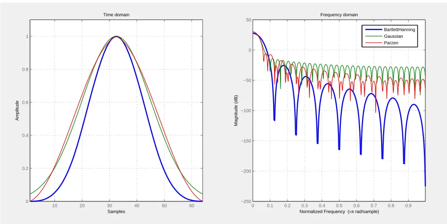
2.1 Lag and spectral window satisfying Assumption 3 . . . 47
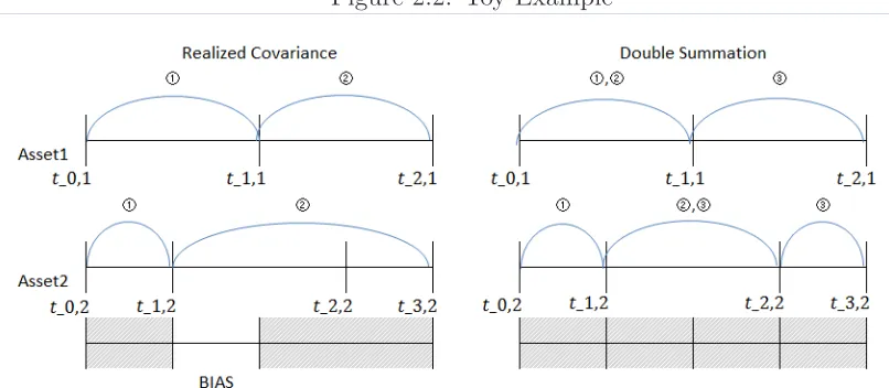
2.2 Toy Example . . . 49
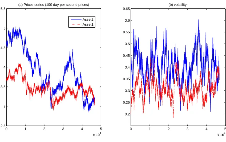
2.3 Simulated intraday instantaneous co-volatility and variance . . . 62
2.4 Simulated price and variance - per second observation . . . 63
2.5 Covariation signature plot . . . 65
2.6 Time stamps of two assets traded at opposite liquidity . . . 66
2.7 Simulation Result : Balanced, Sampled at {3/2,30} . . . 102
2.8 Simulation Result : Unbalanced, Sampled at {3/2,30} . . . 103
2.9 Simulation Result : Unbalanced, Sampled at {20,30} . . . 104
2.10 Simulation Result : Unbalanced, Sampled at {3/2,2} . . . 105
2.11 Covariation matrix estimates : element (1,1) to (2,5) . . . 106
2.12 Covariation matrix estimates : element (3,3) to (5,5) . . . 107
3.1 Time series plot of transaction marks . . . 126
3.3 Sample autocorrelaiton function of activity variables . . . 127
3.4 Sample cross - correlation function of activity variables . . . 127
3.5 Return spaced by equal elapse of financial time, n= 100 . . . 128
3.6 Return spaced by equal elapse of financial time, n= 500 . . . 128
Chapter 1
Realized Volatility: theory and
application
1.1
Introduction
of interest is the integrated variance and its multivariate counterpart. We describe the measurement of these parameters under ideal circumstances and when the data are subject to measurement error. We discuss the main types of measurement error models that apply and how they may arise from the way the market operates at the fine grain, i.e., microstructure issues. We also describe some common applications of this literature. Our review is necessarily selective and there are many topics and papers that we do not cover.
1.2
Modeling Framework
1.2.1
Efficient price
We start by setting the modeling framework. Under the standard assumptions that the return process does not allow for arbitrage and has a finite instantaneous mean, the asset price process, as well as smooth transformations thereof, belong to the class of special semi-martingale processes, as detailed by Back (1991). If, in addition, it is assumed that the sample paths are continuous, we have the Martingale Representation Theorem (e.g. Protter (1990) ). Specifically, there exists a representation for the log price Yt, such that for all t∈[0, T],
Yt=
Z t
0
µudu+
Z t
0
σudWu, (1.1)
where µu is a predictable locally bounded drift, σu is a c´adl´ag volatility process and Wu is an independent Brownian motion, and the integral is of the Itˆo form. Let Ytj
[0, t] is given by
[Y, Y]t= plim
suptj∈Γt|tj−tj−1|→0
X
0≤tj≤t
(Ytj −Ytj−1)
2, (1.2)
with [Y, Y] = [Y, Y]1. This quantity is a measure of ex-post volatility. Under (1.1),
the following holds almost surely
[Y, Y] =
Z 1
0
σu2du. (1.3)
The quadratic variation is also called the integrated variance, for obvious reasons. It is the key parameter of interest that this survey will focus on. It is an integral over the sample path of the stochastic process σ2
u, and hence itself is a random variable. The specification of the process σ2
u is very general and nonparametric, i.e., it may depend on the entire past ofYtand additional sources of randomness. The averaging inherent in (1.3) suggests gains in terms of estimability.
We now relate the parameter of interest to other concepts of volatility. A natural theoretical notion of ex-post return variability in this setting is notional volatility, Anderson, Bollerslev, Diebold, and Labys (2000). Under the maintained assumption of continuous sample path, the notional volatility equals the integrated volatility. The notional volatility over an interval [t−h, t], is
υ2(t, h)≡[Y, Y]t−[Y, Y]t−h =
Z t
t−h σ2udu.
var (Yt|Ft−h) ≡ E
{Yt−E(Yt|Ft−h)}2|Ft−h
= E
"Z t
t−h
µudu−E
Z t
t−h
µudu|Ft−h
+
Z t
t−h
σudWu
2
|Ft−h
#
= E
"Z t
t−h{
µu−E(µu|Ft−h)}du
2 |Ft−h # (1.4) +E "Z t
t−h
σudWu
2
|Ft−h
#
(1.5)
+2E
Z t
t−h{
µu−E(µu|Ft−h)}du
Z t
t−h
σudWu|Ft−h
. (1.6)
Denote Ah = Oa.s.(Bh) when Ah/Bh converges almost surely to a finite constant as h → 0. We have that (1.4)= Oa.s.(h2), (1.5)=
Rt t−hσ
2
udu = Oa.s.(h), and (1.6)= Oa.s.(h3/2), so that (1.5) is the dominant term. Therefore, we have
var (Yt|Ft−h)≃E[υ2(t, h)|Ft−h].
In other words, the conditional variance of returns volatility is well approximated by the expected notional volatility, i.e., it is an approximately unbiased proxy. The above approximation is exact if the mean process,µu = 0, or ifµu is measurable with respect toFt−h. However, the result remains approximately valid for a stochastically evolving mean return process over relevant horizons, as long as the returns are sampled at sufficiently high frequencies. This gives further justification for [Y, Y] as a parameter of interest.
Notional volatility or integrated volatility is latent. However, it can be estimated consistently using the so-called Realized Volatility. The Realized Variance (RV) for the time interval [0,1] is the discrete sum in (1.2);
[Y, Y]n = n
X
j=1
(Ytj−Ytj−1)
where t= 1.
Barndorff-Nielsen and Shephard (2002) showed that the RV is a √n consistent estimator of the QV and is asymptotically mixed Gaussian under infill asymptotics. We can also generalize the above specification for the process driven by L´evy process. In this case the Realized Variance converges in probability to the quadratic variation of the process, which includes contributions from the jumps. We discuss estimation further below.
1.2.2
Measurement error
Empirical evidence suggests that the price process deviates from the semimartingale assumption in (1.1). The “volatility signature plot” (which shows (1.7) against sam-pling frequency) in Figure 1.5 suggests a component in observed price that has an infinite quadratic variation. Previous authors have identified this component as mi-crostructure noise, meaning that it is due to the fine grain structure of how observed prices are determined in financial markets. A common way of modeling this is as follows. Let Xtj be an observed log price and Ytj be discretely sampled from the
process in (1.1). Then suppose that
Xtj =Ytj+εtj, (1.8)
where εtj is a random error term. The simplest case is where the microstructure
noise εtj is i.i.d. with zero mean, independent of the process Y. This model was first
considered in Zhou (1996). In this case, Zhang, Mykland, and A¨ıt-Sahalia (2005) showed that RV = 2nE(ε2) +Op(n1/2), which implies that RV is inconsistent and
Also to closely mimic the high frequency transaction data authors considered rounding error noise or non-additive noise that is generated from specific model of order book dynamics. Li and Mykland (2007) discuss the rounding model,
Xtj = log(δ[exp(Ytj+εtj)/δ])∨logδ, (1.9)
where δ[s/δ] denotes the value of s rounded to the nearest multiples of δ which is a small positive number. This is consistent with the market that has a minimum price change, tick sizes for stocks and futures and pips for foreign exchange. The rounding model (1.9) is much more complex to work with than (1.8), due to the nonlinear way in which the efficient price enters. For example, even assuming no microstructure noise the quadratic variation ofXtis given by [f(Y), f(Y)]t wheref(Y) =E(X|Y) is a complicated nonlinear function, although we are interested in estimating [Y, Y]t. Li et al. (2007) showed that when var(ε) is large, we havef(Yt)≃Yt, whereas for a small noise variance, the divergence of two quadratic variations can be large. In any case, under the presence of such microstructure noise the Realized Variance is no longer a consistent estimator of the integrated variance. We explore the impact of different microstructure noise assumptions on RV and the class of consistent estimators under (1.1) and (1.8) in Section 1.4.
1.3
Issues in Handling Intra-day Transaction
Data-base
Figure 1.1: Time series of intra-day price, trade duration and volume over a day
0 2000 4000 6000 8000 10000 12000 36.5
37 37.5 38 38.5 39
Time series plot of intra−day prices
0 50 100 150 200 250 300 350 400 450 500 37.6
37.65 37.7 37.75 37.8 37.85 37.9 37.95 38 38.05 38.1
Zoomed−in
0 0.5 1 1.5 2 2.5x 10
4
Trade duration
0 0.5 1 1.5 2 2.5x 10
4
Volume of excuted trade trade
bid ask
with finite second moment but with large fourth moment and the tail of the distribu-tion declines according to a power law. In fact, prices are discrete, taking values that are integer multiples of tick sizes, which vary according to assets and time period (in the US stock market tick size changed from being 1/8 of a dollar to 1/100 of a dollar during a few years at the beginning of the last decade), see Figure 1.1 which plots intra-day price of the Dell stock over a single day. The data we use in this paper is a National Best Bid and Offer (NBBO) trade and quote consolidated dataset from TAQ. This puts together the best available quotes from multiple venues and matches the trades to NBBO quotes. Therefore, trade and quote price dynamics should be indicative of that from the single order book. However, returns, whether defined log-arithmically or exactly, are less discrete, since the normalization changes over time, so this comment mostly just affects the study of prices within a single day.
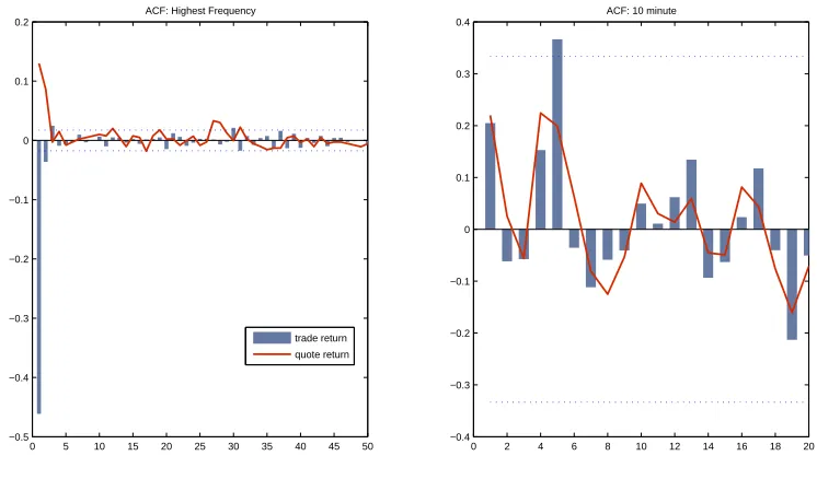
Figure 1.2: ACF of trade and quote returns at different sampling frequency
0 5 10 15 20 25 30 35 40 45 50 −0.5
−0.4 −0.3 −0.2 −0.1 0 0.1 0.2
ACF: Highest Frequency
0 2 4 6 8 10 12 14 16 18 20 −0.4
−0.3 −0.2 −0.1 0 0.1 0.2 0.3 0.4
ACF: 10 minute
trade return quote return
and Bollerslev (1997) showed that the absolute trade returns, after eliminating the short term periodic component, have an hyperbolic decaying autocorrelation function. This can affect the construction of the standard errors and forecasting. Variables as-sociated with transaction activity show periodic patterns due to trading convention. Activities are high at the start and at the end of the trading session and this induces a particular pattern in activity variables. See bottom left of Figure 1.1. Periodicity can be modeled by introducing periodic dummies, frequency domain filtering and analysis at the activity time scale. The intra-day periodicity and long memory structure can be explained by the presence of the information arrival process that drives the price formation process.
1.3.1
Which price to use?
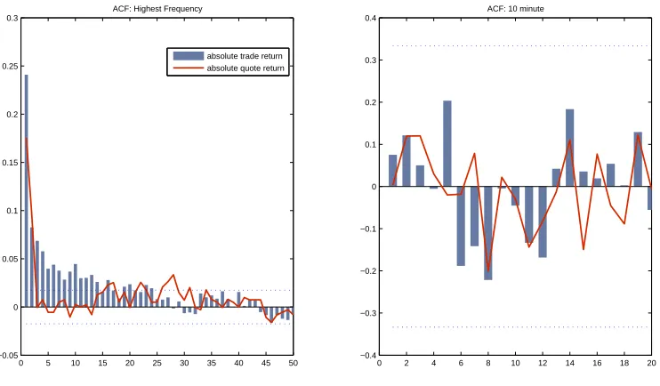
Figure 1.3: ACF of absolute trade and quote returns at different sampling frequency
0 5 10 15 20 25 30 35 40 45 50 −0.05
0 0.05 0.1 0.15 0.2 0.25 0.3
ACF: Highest Frequency
0 2 4 6 8 10 12 14 16 18 20 −0.4
−0.3 −0.2 −0.1 0 0.1 0.2 0.3 0.4
ACF: 10 minute absolute trade return
absolute quote return
of order book and also the volumes of these orders. We may construct such price as a weighted sum of quote prices at different levels of order book where weight is given by the associated volume. Such price construction has the advantage that it uses more information available regarding investor’s anticipation of price movement and discreteness is less severe by construction. Related but not the same VWAP (volume weighted average price) can be also used. Over specified period, it is constructed by taking sum of executed trade price weighted by its volume. This quantity is used in a common strategy for execution of large transactions, see Almgren and Chriss (2001) for example.
One of the important conclusions we can draw from the analysis is that in ultra-high frequency, the choice of quote or trade price will sometimes affect the results of empirical modeling. For example, in calculating the naive Realized Variance measure of integrated variance based on low frequency returns, at 10-20 minutes which is a popular choice, the choice of quote or trade returns will not have a discernible impact on the final quantity. However for more recently proposed methods that use un-sampled tick data, we should compare the results using quote and trade returns. See Barndorff-Nielsen, Hansen, Lunde and Shephard (2008b) for such studies.
1.3.2
High frequency data pre-processing
Prior to analysis, the tick data has to be pre-processed to remove non sensible prices and duplicated transaction data points. Barndorff-Nielsen et al. (2008b) provide a guideline to do this for equity intra-day data. Brownlees and Gallo (2006) summa-rize the structure of the TAQ high frequency dataset and address various issues in high frequency data management including: outlier detection and how to treat non-simultaneous observations, irregular spacing, issues of bid-ask bounce, and methods for identifying exact opening and closing prices. The authors also present the effect of data handling on the result of empirical analysis.
on NYSE traded stocks and major currencies. Empirical application in other markets - geographically and also other fixed income markets will be of interest.
1.3.3
How to and how often to sample?
Intra-day prices are observed on the discrete and irregular intervals. For volatility estimation one can ask what is the effect of using all the data versus using sparsely sampled data, for example at 10-20 minutes. For covariance estimation, the problem is more substantial. Naturally the estimation of covariance involves the cross product of returns. How should we align the data points observed at a different times and what is the statistical impact of the synchronization method on the estimators? This section discusses two data sampling/alignment method: fixed clock time and refresh time method. We will present the synchronization method for d number of assets. The sampling method for univariate series is a special case for d = 1. In a given interval (for simplicity one day) [0,1], we observe intra-day transaction prices of the i-th asset, Xi at discrete time points {ti,j;j = 0, . . . , ni} where ni is a total number of observations on that interval. The set of
{Xi,ti,j, ti,j;i= 1,· · · , d, j = 1, . . . , ni},
gives us the tick database of prices for d numbers of assets. We can associate the counting process to {ti,j}
Ni(t) := ni
X
j=1
1(ti,j ≤t),
recording the number of transactions that occurred for the i-th asset up to and in-cluding the time t. Let 0 = τ0 < · · · < τn = 1 be an artificially created time grid and let {si,j} be the actual time points of the data fori-th asset to be aligned on the
{τj}’s grid. Regardless of how τ is defined we take the data that is closest to this artificial grid,
si,j = max
0≤l≤ni{
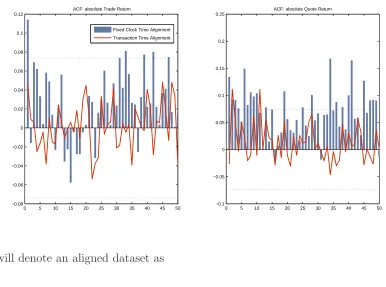
Figure 1.4: ACF of absolute trade and quote returns sampled by fixed clock time and transaction time
0 5 10 15 20 25 30 35 40 45 50 −0.08
−0.06 −0.04 −0.02 0 0.02 0.04 0.06 0.08 0.1 0.12
ACF: absolute Trade Return
0 5 10 15 20 25 30 35 40 45 50 −0.1
−0.05 0 0.05 0.1 0.15 0.2 0.25
ACF: absolute Quote Return Fixed Clock Time Alignment
Transaction Time Alignment
We will denote an aligned dataset as
{Xi,τj, τj;i= 1,· · · , d, j = 1,· · ·, n},
with Xi,τj :=Xi,si,j. If no observation is available during the given interval we repeat
the previous data point.
First, consider the problem of sampling scheme for univariate time series of intra-day prices. One can use the raw tick data of prices observed at {ti,j} or work with instead sparser sampling. One method of sparse sampling is called fixed clock time. For example, we might want to create one minute returns from the irregularly spaced tick data
τj =jh ,h = 1/60, (1.10)
so thatτj−τj−1 =h,for alli. Empirical work shows that the effect of microstructure
microstructure noise is present but unaccounted for, they showed that the optimal sampling frequency is finite and derived its closed-form expression. The optimal sampling frequency is often found to be between one and five minutes. See Bandi and Russell (2008) and reference therein for further discussion of the optimal sampling rate in estimating integrated variance. However, modeling the noise and using all the data should yield a better solution, see Section 1.4.1. on the noise robust estimators. The second method for sparse sampling is to sample the price per given number of transactions. For example, data sampled per h number of transactions is
τj+1 =ti,Ni(τj)+h. (1.11)
Griffin and Oomen (2008) argued that under the transaction time sampling, returns are less serially correlated and microstructure noise is closer to i.i.d. They note the bias correction procedures that rely on the noise being independent are better implemented in transaction time. Figure 1.4 shows that the ACF of absolute returns at a different sampling scheme - verifying that the transaction time sampling scheme reduces the serial correlation and the process is closer to i.i.d.
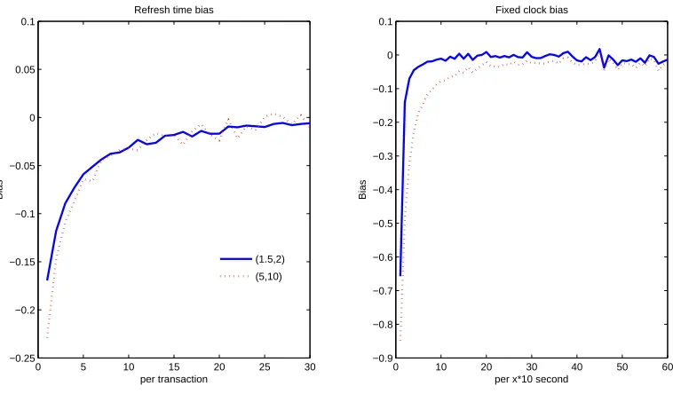
For the multivariate case, the additional issue of synchronicity arises, whereby trading for different assets occurs at different times. It is necessary to align the returns of asynchronously traded assets to calculate the covariance estimator that involves the cross product of returns. One method is to use the fixed clock time as given in (1.10). Another method, called the Refresh time, proposed by Barndorff-Nielsen, Hansen, Lunde and Shephard (2011) can be thought as the multivariate version of the transaction time alignment given in (1.11). It is constructed by
τj+1 = max
Figure 1.5: Realized variance calculated at different calendar time frequencies
0 5 10 15 20 25 30 35 40 45
0 0.002 0.004 0.006 0.008 0.01 0.012
Sampling frequency
Realized Variance
covariance estimation since the method effectively collects the transaction time of the most illiquid asset. See Zhang (2010) for further studies on the refresh time bias and its effect on the time domain based estimator of integrated covariance matrix. See Section 1.4.2 for a discussion of covariance estimator robust to the synchronization bias.
1.4
Realized variance and covariance
1.4.1
Univariate volatility estimators
We first present the results for realized volatility in the perfect world where there is no measurement error. The case of no noise is dealt with by Andersen, Bollerslev, Diebold and Labys (2001), Barndorff-Nielsen and Shephard (2002), and Mykland and Zhang (2006). Barndorff-Nielsen et al. (2002) showed that the error using the RV to estimate the QV is asymptotically normal with rate √n, i.e.,
√
n
P
jyt2j −
R1
0 σ
2
udu
q
2R01σ4
udu
whereytj =Ytj−Ytj−1 is the observed return and =⇒denotes convergence in distribu-tion. We remark that their proof does not require that Ey4
tj <∞ or even Ey
2
tj <∞
as would generally be the case for a central limit theorem to hold. The reason is that the data generating process assumes a different type of structure, namely that locally the process is even Gaussian, and it is this feature that permits the arrival of the normal distribution in the limit. Note that this CLT is statistically infeasible since it involves a random unknown quantity called integrated quarticity (IQ), R01σ4
udu. However we can consistently estimate this by the following sample quantity
c
IQ= n 3
X
j
y4tj →p IQ.
Therefore, the feasible CLT is given by
√
n
P
jyt2j −
R1
0 σ
2
udu
q
2IQc
=⇒N(0,1).
This implies that Pjy2
tj ±zα/2
q
2 3
P
jy4tj gives a valid α-level confidence interval for
R1 0 σu2du.
Measurement Error
Motivated by some of the issues observed in the intra-day financial time series largely to do with the presence of microstructure noise, authors have proposed competing estimators of the QV. The assumption on a microstructure noise has been generalized from a white noise to a noise process with some of following characteristics: autocor-relation, heteroscedasticity, rounding models. McAleer and Medeiros (2008) provide a summary of the theoretical properties of different estimators of QV under different assumptions of microstructure noise.
containing ni observations. Let [X, X]ni denote theith subsample estimator based on a K-spaced subsample of size ni, and let [X, X]avg denote the averaged estimator:
[X, X]ni =
nXi−1
j=1
XtjK+i−Xt(j−1)K+i
2
, i= 1, . . . , K,
[X, X]avg = 1 K
K
X
i=1
[X, X]ni.
To simplify the notation, we assume thatnis divisible byK and hence the number of data points is the same across subsamples, n1 =n2 =...=nK =n/K. Letn =n/K. Define the adjusted TSRV estimator as
\
[X, X] = [X, X]avg −
n n
[X, X]n. (1.13)
Zhang et al. (2005) show that this estimator is consistent and show that
n1/6[\X, X]−[X, X]
q
8c−2E2ε2+ 4
3cIQ
=⇒N(0,1),
provided that K =cn2/3 for any c∈(0,∞).Zhang (2006) extended this work to the
multiscale estimator (MSRV). She shows that this estimator is more efficient than the two time scale estimator and achieves the best convergence rate ofOp(n1/4),(i.e., the
same as the MLE with complete specification of the observed process).
Kalnina and Linton (2008) proposed a modification of the TSRV estimator that is consistent under heteroscedasticity and endogenous noise. A¨ıt-Sahalia, Mykland and Zhang (2010b) modified TSRV and MSRV estimators and achieve consistency in the presence of serially correlated microstructure noise.
Bartlett (1946). Define the symmetric realized autocovariance sequence
γh(X) := n
X
j=h+1
xtjxtj−h, (1.14)
for h ∈ Z+ and γ
−h(X) = γh(X). At a zero lag, γ0(X) gives us the usual sum of
squared high frequency returns, i.e., RV. The kernel estimators smooth the realized autocovariances with the weight function given by k(·), where k(0) = 1, k(s) → 0 as s → ∞ and the bandwidth H controls the bias-variance trade-off. Specifically, consider
\
[X, X] = X |h|<n
k
h H+ 1
γh(X). (1.15)
Zhou (1996) was the first to consider the use of the kernel method to deal with the problem of microstructure noise. Hansen and Lunde (2006) examined the properties of Zhou’s estimator and showed that, although unbiased under the presence of i.i.d microstructure noise, the estimator is not consistent. However, they advocated that, while inconsistent, Zhou’s kernel method is able to uncover several properties of the microstructure noise.
Barndorff-Nielsen et al. (2011) proposed an estimator of the form in (1.15) with a second order kernel k(·). Their important contribution is to show that it is consis-tent under the presence of second order stationary noise, and that furthermore, it is asymptotically normal with rate Op(n1/5) and
n1/5[\X, X]−[X, X]−c−2|k′′(0)|w2
p
4c||k||2IQ =⇒N(0,1), (1.16)
provided that H = cn3/5 for c ∈ (0,∞), where ||k||2 := R∞
−∞k(s)2ds and w2 =
P
estimator of Barndorff-Nielsen and Shephard (2004b) which is guaranteed to be posi-tive definite but rate inefficient atOp(n1/5). In Barndorff-Nielsen et al. (2008a), they
had a realized kernel estimator with a flat-top kernel i.e. k(0) =k(|1|/H) = 1 and the realized autocovarianceγhwas defined such that the sum runs from 1 noth+1. Their flat top realized kernel is unbiased under the presence of i.i.d microstructure noise and achieves the optimal convergence rate, Op(n1/4). The drawback of the earlier
version, however is that the resulting estimator is not guaranteed to be p.s.d.
We should briefly mention the promising pre-averaging method analyzed for ex-ample in Jacod, Li, Mykland, Podolskij and Vetter (2009), which involves averaging observed prices over a moderate number of time points to reduce the measurement error. Consider
Xt= 1 nt
X
|t−tj|<ǫT
Xtj ; xt =
1 nt
X
|t−tj|<ǫT
xtj,
wherentis the number of time points with |t−tj|< ǫT for some smallǫT →0.Then Xt=n−t1
P
|t−tj|<ǫT Ytj +Op(n
−1
t ) andxt =n−t1
P
|t−tj|<ǫTytj +Op(n
−1
t ), so that now the noise is small provided nt is large. The preaveraged data can then be used in a variety of the above procedures.
The final method involves a little departure. Parkinson (1980) and Alizadeh, Brandt and Diebold (2002) proposed a range-based volatility proxy defined by the extreme prices over the pre-determined interval. Specifically, let
R= sup
0≤t≤1Xt−0≤inft≤1Xt.
This is an alternative measure of volatility to QV. In some special cases it has a known positive relationship with QV. Specifically, if Xt = σWt, then R is a stochastic variable, while the quadratic variation is the constant σ2. In fact, R =
σsup0≤u≤1W(u)−inf0≤u≤1W(u)
, from which one can compute ERκ =λ
κσκ/2 for κ ≥ 1, where λκ are known constants. More generally the relationship between R and QV is likely to be rather complex. In practice, one may compute
Rn= max
from a given sample of data observed at timest1, . . . , tn.One can expect thatRn → R with probability one under quite general conditions. The most rigorous analysis of the realized range has been in Christensen and Podolskij (2007), except that they only compute R over small subintervals, which is like assuming that locallyXt=σWt for someσ, and then average the resulting values ofRnover these subintervals. Alizadeh et al. (2002) recommend using the log of the sample range, as it is closer to a normally distributed random variable.
The realized range has the significant advantage that one can find the daily value in the newspapers for a variety of financial instruments, and so one has a readily available volatility measure without recourse to analysis of the intra-day price path. Alizadeh et al. (2002) also argue that the method is relatively robust to a measurement error of a bid-ask bounce variety, since the intra-day maximum is likely to be at the ask price and the daily minimum at the bid price of a single quote and so one expects a bias corresponding only to an average spread. By contrast, in computing the realized variance one can be cumulating these biases over many small periods, thereby greatly expanding the total effect.
A number of authors have carried out empirical studies to rank the performance of competing estimators of QV. One way to do this is by simulating the process given in (1.1). To test for the robustness of the estimator, we may introduce jumps in the price or in the volatility, assume different settings for microstructure noise or sampling scheme. Gatheral and Oomen (2010) took a different approach to this and simulated the order book directly. They compared QV estimators under the realistic microstructure setting and compared if the theoretical prediction matches well with actual small sample properties. They found that subsampling estimator, realized kernel, and maximum likelihood estimator deliver superior performance in terms of efficiency and robustness to different parameterizations of microstructure noise.
al. (2008b) for example. Authors also compared forecasts of QV estimators under different scenarios of underlying stochastic volatility process and the distribution of microstructure noise. A¨ıt-Sahalia and Mancini (2008) found that TSRV in (1.13) outperforms the RV under varying degree of assumptions. Bandi, Russel and Yang (2008) considered comparison in the context of option pricing and Voev (2009) in the context of an unconditional measure of portfolio performance.
1.4.2
Multivariate volatility estimators
In this section we discuss estimators of integrated covariance matrix. We present a framework for the bivariate case, as this allows treatment of the main issues. We suppose that the efficient price process follows a Brownian semimartingale. For the i-th asset, i= 1,2, we have
Yi,t =
Z t
0
µi,udu+
Z t
0
σi,udWi,u, (1.17)
where µi,u is a predictable locally bounded drift, σi,u is a c´adl´ag volatility process, andWi,uis a Brownian motions withE[dW1tdW2t] =ρtdt. The time span we consider is fixed and scaled to vary between [0,1]. We observe a (log) price at discrete time points, 0 = ti,0 < · · · < ti,ni = 1. Let Υ be a set of points that partition the
interval [0,1]. Define mi(n) := supj:ti,j∈Υ|ti,j−ti,j−1| and assume that as n → ∞,
m(n) := m1(n)∨m2(n) → 0, so that the observation grid is becoming finer and
finer. Denote by Yi,ti,j the discretely sampled log prices. Suppose that the two prices
series are observed on the synchronous time points {τj, j = 1, . . . , n}. The quadratic co-variation of Y1 and Y2 over a time interval [0,1] is defined by
[Y1, Y2] = lim
m(n)→0
n
X
j=1
(Y1,τj−Y1,τj−1)(Y2,τj−Y2,τj−1) =
Z 1
0
σ1,uσ2,uρudu, (1.18)
of quadratic co-variation is the discrete sum in (1.18), called the Realized Covariance
[Y1, Y2]n =
n
X
j=1
(Y1,τj−Y1,τj−1)(Y2,τj −Y2,τj−1). (1.19)
Under perfect synchronization, Barndorff-Nielsen and Shephard (2004a) showed that the Realized Covariance is a√n consistent estimator of the integrated covariance and is asymptotically mixed normal under (1.17). Let us denote the returns for the i-th asset by yi,τj :=Yi,τj −Yi,τj−1. Then, we have
√
n
Pn
j=1y1,τjy2,τj−
R1
0 Σ1,2(u)du
qR1
0 Σ1,1(u)Σ2,2(u) + (Σ1,2(u)) 2
du
=⇒N(0,1).
The corresponding feasible CLT is given by
Pn
j=1y1,τjy2,τj −
R1
0 Σ1,2(u)du
qP
jy12,τjy
2 2,τj−
P
jy1,τjy1,τj+1y2,τjy2,τj+1
=⇒N(0,1).
Compare this with the univariate case in the previous section. A similar asymp-totic argument can be carried out for the realized regression coefficient or the realized betas in the capital asset pricing model (CAPM).
The time stamp for transactions of two different securities rarely matches, and so some data synchronization method is typically employed. This will have an impact on the finite sample as well as on the asymptotic behavior of the resulting covariance estimate. The well known Epps effect refers to the phenomenon that the sample cor-relation tends to have a strong bias towards zero as the sampling interval progressively shrinks. Hayashi and Yoshida (2005) showed that the realized covariance calculated from the aligned data using the fixed clock time alignment method described in the Section 1.3.3 is biased. They proposed a modified covariance estimator
\ [Y1, Y2] =
n
X
i=1
n
X
j=1
which they show is unbiased and√nconsistent. Under presence of asynchronicity but with no microstructure noise this estimator is theoretically the best one. Essentially their estimator takes the cross product of returns only if the portion of transaction time intervals of two assets overlaps.
Malliavin and Mancino (2009) proposed an estimator of the integrated covariance that does not require synchronization. They establish the relationship between the Fourier transform of returns and the Fourier transform of spot volatility. Under (1.17), their estimator is consistent and asymptotically normal. Their estimator is defined by
\ [Y1, Y2] =
1 2m+ 1
X
|k|≤m
Fn(Y1)(k)Fn(Y2)(−k),
where Fn(Yi)(·) denotes the discretized Fourier transform of i-th asset returns. For k ∈Zand assuming that the time interval is re-scaled to vary [0,2π],
Fn(Yi)(k) := n
X
j=1
eikti,j(Y
i,ti,j−Yi,ti,j−1)→p
Z 2π
0
eiktdYt.
In fact, they have a stronger result where the Fejer Fourier inversion of the above estimator gives a consistent estimator of the instantaneous (co)volatility.
Finally, we should mention some work on the multivariate range based estimation. Brandt and Diebold (2006) extended the work on the realized range to the multivari-ate case. It is not immedimultivari-ately obvious how to extend such notion to the multivarimultivari-ate case, and indeed their cunning idea relies on the specific structures that arise in a number of settings, notably exchange rates. Suppose we observe the exchange rates between three currencies: A, B,andC,denotedXA:B, XB:C,andXA:C,then we know that in the absence of arbitrage XA:C =XA:BXB:C. Taking logs and differencing, we obtain
cov(∆ lnXA:B,∆ lnXA:C) =
1
method as before is that it does not require high frequency data so that the effect of measurement error is minimized.
Measurement Error
So far we have considered the case where the only source of error is observation error, i.e., discretization error of the continuous semimartingale and the non-synchronicity of the observed price. We next consider the presence of an infinite quadratic variation component in the observed prices due to a further measurement issue, microstructure noise. There has not been a uniform approach to modeling multivariate microstruc-ture noise, perhaps due to the confounding effects of asynchronicity. Furthermore, it is not clear if the microstructure noise between two assets should be correlated and if so how to parameterize this quantity. Let us assume an additive noise for each asset
Xi,ti,j =Yi,ti,j +ǫi,ti,j fori= 1, . . . , d,0 = ti,0 < ti,1 <· · ·< ti,ni = 1.
Zhang (2010) assumed that{ǫ1,t1,j, ǫ2,t2,j}are stationary and exponentially alpha
mix-ing. She proposed a Two Scales Realized Covariance estimator (TSCV), which is defined as a bivariate version of (1.13) applied to an aligned data,
\
[Y1, Y2] = [Y1, Y2]K−
nK nJ
[Y1, Y2]J,
where the average lag K realized covariance is defined by
[Y1, Y2]K =
1 K
n
X
j=K
(Y1,τj−Y1,τj−K)(Y2,τj −Y2,τj−K),
for 1 ≤ J ≪ K. Let summation of sample sizes of two assets as N = n1 +n2
and recall that the number of points for the aligned time stamp τ is n. Define nK = n −K + 1)/K and similarly for nJ . Then the above estimator is Op(n1/6) consistent and asymptotically normal under the presence of noise and asynchronous trading, provided that K =O(N2/3).
usingrefresh Time explained in Section 1.3.3. They assumed that the microstructure noise {ǫi,τj, i = 1, . . . , d} is a second order stationary process with respect to refresh
time{τj}. Their Multivariate Realized Kernels (MRK) is given in (1.15) with realized autocovariance defined by
γh(X) =
X
j xτjx
T
τj−h, h= 0,±1,±2,· · ·
where Pj =Ph<j≤n forh≥0, and Pj =P1≤j≤n+h for h <0 and x= [x1 :· · ·:xd] is a matrix of refresh time aligned returns for d number of assets. The MRK is Op(n1/5)−consistent and asymptotically normal and its asymptotic distribution is
given in (1.16) modified with relevant multivariate quantities, under the second order kernel. It is also guaranteed to be positive semi-definite at the cost of asymptotic bias. Note that the asymptotic rate is based on the sample size of the aligned time stamp. A¨ıt-Sahalia, Fan and Xiu (2010a) proposed an Op(n1/4) consistent estimator based on the quasi-MLE and a generalized time synchronization method. An advan-tage of their estimator over TSCV and MRK is that it does not involve choosing or estimating tuning parameters such as bandwidth. However they adopt a somewhat restrictive assumption on the microstructure noise - it is a white noise that is mutually independent across assets.
1.5
Modeling and Forecasting
We will designate the class of estimators of quadratic (co) variation based on the high frequency data as “realized measures”. In this section, we review how realized measures can be used to model and forecast the (co)variances. We will summarize the studies that compare these competing models in terms of forecasting power where the forecasting variable is a general function of volatility such as Value at Risk and portfolio performance. We also consider extensions to a dynamic model of the realized covariance matrix.
1.5.1
Time series models of (co) volatility
There is a large literature on time series models of volatilities. In the well-known GARCH and Stochastic volatility family of models, volatility is treated as a latent variable. The method we discuss here takes a different stance. We treat the Realized Variance as ex-post observed variance. Given the sequence of RVs (or the robust estimator discussed in Section 1.4.1), we use traditional time series techniques such as ARMA to fit a model and carry out forecasts. The key feature of the time series of the Realized Variance is that it is highly persistent. To account for this, Andersen, Bollerslev, Diebold, and Labys (2003) proposed an autoregressive fractionally inte-grated moving average (ARFIMA) to model the time series of the Realized Variance. Let ht denote an estimator of integrated variance for t-th day, t = 1, . . . , T. The ARFIMA model for ht is given by
Φ(L)(1−L)ν(ht−µ) = Θ(L)ǫt, ǫt∼WN(0,1), (1.20)
model. A simpler model that seems to capture lag dependencies well is the Heteroge-nous Autoregressive model of Corsi (2009);
ht+1 =θ0+θDht+θWht(W)+θMh(tM)+ǫt+1, (1.21)
whereh(tW):= 15(ht+· · ·+ht−4) is a Realized Variance over a week and similarly defined
h(tM) denotes a Realized Variance over a month. Shephard and Sheppard (2010) who proposed a model that is a hybrid of a GARCH augmented with a realized measure and a reduced form time series model for the Realized Variance. See similar approach in Hansen, Huang and Shek (2011) who jointly modeled returns and realized measures of volatility. Liu and Maheu (2009) carried out Bayesian averaging over both different measures of integrated variance and different time series models.
In the multivariate setting, a key issue is that the fitted model should produce a positive definite covariance matrix. Also, if we were to model a high dimensional covariance matrix, we need to address the dimension issue, which grows rapidly with the number of assets considered. Voev (2007) proposed a method to combine volatil-ity and bivariate co-volatilvolatil-ity forecasts to produce a positive definite matrix. The problem with this method is that interaction between elements of covariance matrix is not taken into account. The full joint modeling of covariance matrix is an im-portant issue. For example, the variance of one asset and covariance with another asset have significant dependencies, especially during episodes of market crashes and large economic events. Compared with the univariate volatility modeling literature, such multivariate models have been sparsely researched mainly due to the fact that consistently estimating a general d×dcovariance matrix for d >2 has been difficult, plagued by bias induced by synchronization as well as microstructure noise. However with recent work in Section 1.4.2 this area of research can progress further.
m=d(d+ 1)/2. A range of transformation functiong(·) is considered for the purpose of dimension reduction and to guarantee a p.s.d. matrix forecast. We will discuss this in a moment. First consider the vector ARFIMA model
Φ(L)D(L)(ht−BZt) = Θ(L)ǫt, ǫt∼WN(0, Im), (1.22)
where Θ(L) = Im −Θ1L· · · −ΘqLq is a matrix lag polynomial of degree q ∈ Z for
the MA component, Φ(L) is defined similarly for AR component. D(L) =diag{(1− L)ν1, . . . ,(1 −L)νm} is a matrix fractional difference operator with ν
1, . . . , νm the degrees of fractional integration for each element of ht. Zt are exogenous variables that affect the dynamics of volatility; candidate variable are trading activity variables and macroeconomic state variables. B is a restriction matrix. We can estimate such a model by maximum likelihood. The one step ahead prediction is then bht+s = E(ht|hs, s ≤ t). We obtain a covariance matrix forecast by Hbt+s = vech−1(bht+s))
where the vech−1(·) re-stacks the vector into a symmetric matrix.
Bauer and Vorkink (2011) fitted the vech of log(Ht) (rather like a matrix E-GARCH model) to an AR model where the right hand side lagged variables are dimension reduced by principal component analysis. Chiriac and Voev (2011) carried out a Cholesky decomposition of the covariance matrix and model the lower dimen-sional factors by a vector ARFIMA model. They showed this method outperforms in terms of root mean square error, a number of models including: the Heteroge-neous Autoregressive model, a multivariate version of (1.21), Wishart Autoregressive (WAR) model of Gourieroux, Jasiak, and Sufana (2009) and the Dynamic Condi-tional Correlation model. We may use the Realized Variance to proxy true Ht+s and compare the Frobenius norm of the bias kHbt+s−Ht+sk, across different models and different horizons s. Authors also compare minimum variance portfolio efficient frontiers using different covariance matrix forecast.
1.5.2
Forecast comparison
robust to the measurement error in the volatility proxy. In the previous section, we presented how we can compare root-MSE of covariance forecasts. We might be interested in economically meaningful loss functions. Brownlees and Gallo (2010) compared the Value at Risk forecasts from different time series models of RV. Bandi et al. (2008) considered the forecast comparison in the context of option pricing.
An important research question is whether there is a gain in using the high fre-quency data over traditional daily volatility models. We can compare the dynamic model of estimators of ex-post variation calculated from the high frequency data against the latent volatility models such as GARCH and Stochastic Volatility. Koop-man, Jungbacker and Hol (2005) found that the ARFIMA model of RV delivers the best out-of-sample forecast compared with the GARCH or the SV model fitted to a daily S&P500 index. Shephard and Sheppard (2010) showed their hybrid model using the realized measures outperforms the daily GARCH model in terms of various criteria. Siu and Okunev (2009) compared historical, realized and implied volatility measures for predicting over multiple horizons.
We are also interested in ranking the competing realized measures in Section 1.4. Ghysels, Santa-Clara and Valkanov (2006) proposed a framework to do this, called the mixed data sampling (MIDAS) regression, comparing measures of ex-post variation in terms of their forecasting ability at various horizons. Ghysels and Sinko (2011) found that the microstructure robust realized measures deliver better forecasts. Likewise, A¨ıt-Sahalia and Mancini (2008) reach similar conclusion where the TSRV estimator in (1.13) outperforms the RV under diverse setting of volatility process and assumptions on the noise.
1.6
Asset Pricing
1.6.1
Distribution of returns conditional on the volatility
measure
(2001) found that daily returns standardized by the realized volatility approximate the Gaussian distribution. Thomakos and Wang (2003) also found such evidence for a futures market.
Peters and de Vilder (2006) studied the volatility and return dependence by sam-pling the returns in financial time. They tested if the return series are a realization of a local martingale using the theorem by Dubins and Schwarz (1965) who stated that any continuous local martingale Yt ∈ Ft is a time-changed Brownian motion. Formally stated,
Bs =YTs , Ts= inf{t|[Y]t ≥s}, (1.23)
where Bs ∈ FTs is an independent Brownian motion and Ts is a stopping times. It
is the first time the quadratic variation reaches a specified level. Equivalently, the theorem implies that
Yt=B[Y]t, (1.24)
which states that every continuous martingale is a time-changed Brownian motion where the time change is given by the quadratic variation. In empirical analysis, (1.23) is more useful, since it states that between the unit interval of the transformed time, [T(j−1)a, Tja], Y has a constant QV at a. Given an interval of physical time, Y is sampled more frequently when QV is large. More precisely, the (discretized) transformed time is constructed by: T0 = 0, T(j+1)a =Tja+ ∆T(j+1)a,
∆T(j+1)a = inf{t|[Y][Tja,Tja+t) ≥a}, (1.25)
where [Y][Tja,Tja+t) denotes the quadratic variation in the interval [Tja, Tja+t). The
standardized increment in financial time
ξ = YTja−YT(j−1)a
√
a , (1.26)
process is completely specified. Testing for the hypothesis thatYtis a local martingale is then equivalent to testing for i.i.d standard normality of the return series that is spaced by Ts. Peters and de Vilders (2006) tested if the S&P500 intra-day return is a local martingale where they constructed the stopping time Ts based on the Realized Variance. They concluded that we cannot reject the null hypothesis that returns are the realization of a martingale process at various time scales (> 1 day) based on the tests for Gaussianity, independence and serial correlation.
1.6.2
Application to factor pricing model
We next discuss applications to asset pricing models for cross-sections of returns. Denote a stock return fori-th firm at timetbyyi,t,withi= 1, . . . , dandt= 1, . . . , T. The K factor pricing model for stock returns is given by
yi,t =βi⊤ft+εi,t, (1.27)
where the factor loadingsβi = (βi,1, . . . , βi,K)⊤are unrestricted. The sampling unittis typically a low frequency such as monthly. In some casesftare unobserved statistical factors, while in others they are the returns on carefully constructed portfolios. In the latter case, βi,k can be given the interpretation of the covariance between return on portfolio k and asset i divided by the variance of the return on portfolio k. The continuous time framework allows us to measure the time varying beta between two assets using the high frequency data. The realized beta between asset i and k in period [t−1, t] calculated from high frequency returns {y·,t} is given by,
ˆ
βi,k(t) =
P
jyi,jyk,j
P
jyk,j2
→p
Rt
t−1Σi,k(s)ds
Rt
t−1Σk,k(s)ds
:=βi,k(t),
can be posed as a GMM estimation problem. They used the Realized Variance as a conditional volatility proxy and showed that there is a significant time-variation in the risk-return slope coefficient. Bali et al. (2006) found a positive and statistically significant relation between the conditional mean and conditional volatility of market returns at a daily level where volatility is proxied by RV. Bollerslev et al. (2006) made use of the time aggregation formula between lower and high frequency covariance. They found that the correlations between absolute high-frequency returns and current and past high-frequency returns are significantly negative for several days.
Andersen, Bollerslev, Diebold and Wu (2005) and Bandi and Russell (2005) esti-mated the beta in CAPM by a realized covariation. Bandi et al. (2005) provided the MSE-based optimal sampling frequency for calculating the realized beta designed to reduce the effect of market microstructure noise. Bollerslev and Zhang (2003) esti-mated the factor loadings in the three-factor Fama-French model using the high fre-quency data adopting a simple adjustment procedure to account for non-synchronous trading effects. Bannouh, Martens, Oomen and van Dijk (2009) and Kyj, Ostdiek and Ensor (2009) used a mixed frequency framework, using the high-frequency data to obtain an estimate of the factor covariance matrix and using the daily data to estimate the factor loadings. This method avoids the non-synchronicity between a individual stock and usually more liquid factor prices.
1.6.3
Effects of algorithmic trading
Recently, the effects of high frequency or algorithmic trading have been the focus of policy discussions, arising part from the flash crash of May 2010, where the US market suffered rapid price decreases followed ultimately by a recovery. Chaboud, Chiquoine, Hjalmarsson and Vega (2009) investigated the effects of algorithmic trading on volatil-ity in the foreign exchange market. They considered the following regression equation
RVit =αi+βiATit+γi⊤τit+
22
X
k=1
δikRVi,t−k+εit,
where RVit is the log of realized volatility of currency i during day t computed us-ing one minute returns, ATit is the fraction of algorithm trading in that day and currency, which was recorded by the trade matching engine, and τit are dummy and time trend variables. The latter are included because theAT series has a pronounced upward trend, while volatility appears to be stationary. They recognized AT is en-dogenous variables since high frequency automated trading algorithms may trade more in volatile times. They therefore instrument it with a variable that measures the capacity for computer trading in a given currency/period combination. The es-timation strategy matters here, so that using OLS yields a positive effect, βi > 0, but the instrumental variable estimator finds βi <0 but not statistically significant. They conclude that intra-day algorithmic trading does not by itself lead to higher daily volatility. For other studies that use realized measure of volatility to determine the effects of high frequency trading, see Hendershott, Jones and Menkveld (2009) and Hendershott and Riordan (2009).
1.6.4
Application to option pricing
volatility swap is swapping a fixed volatility SWt,T for a floating (actual) volatility [Y]t,T, denoting quadratic variation accumulated over [t, T]. The floating leg is usually given by a sum of squared daily log returns over the relevant time interval. Given N notional amount in dollar terms per annualized volatility point, its payoff at expiration is equal to
([Y]t,T −SWt,T)N.
Denote r a risk-free discount rate corresponding to an expiration date T. The value of such forward contract is given by the expected present value of the future payoff under a risk neutral measure Q, a probability measure such that the discounted price of traded asset is a martingale,
EQ[erT([Y]t,T −SWt,T)].
Then the strike for which the contract has zero present value is
SWt,T∗ =EQ([Y]t,T).
Carr, Geman, Madan and Yor (2005) proposed a method of pricing options on quadratic variation via Laplace transform when returns follow pure jump L´evy pro-cess. Itkin and Carr (2010) considered a pricing problem when returns are time changed L´evy processes. Britten-Jones and Neuberger (2000) proposed a method to estimate EQ([Y]T), an option-implied (i.e. risk-neutral) integrated variance over
the life of the option contract, assuming price follows stochastic volatility diffusion process. SWt,T∗ can be labeled as a model-free implied variance as well as being a no-arbitrage variance swap rate. Carr and Wu (2009) showed that the variance swap rate is well approximated by the value of a particular portfolio of options. They estab-lished that the difference between the Realized Variance and this synthetic variance swap rate, given by
[Y]t,T −SWt,T∗ ,
to pay a premium to hedge away upward movement in the return variance.
Bollerslev, Gibson and Zhou (2010) proposed a method for constructing a volatility risk premium relying on sample moments of the Realized Variance and a option-implied volatility estimator. Wu (2010) studied the variance risk premium using both variance swap rates constructed from the option prices and the quadratic variance estimates using the high frequency data and found a strong evidence for negative variance risk premium in the equity market.
1.7
Estimating continuous time models
In this section we review how realized measures can be used to estimate the parameters of a continuous time model. Consider a diffusion model for financial prices Xt,
dXt=µ(Xt, θ)dt+σ(Xt, θ)dBt, (1.28)
whereBtis an independent Brownian motion,µ(Xt, θ) is a drift function andσ(Xt, θ) is a given diffusion coefficient function. We are interested in estimating vector of pa-rameters θ. Xtis non-homogenous in a sense that the diffusion coefficient is not con-stant. This specification includes geometric Brownian motion, Ornstein–Uhlenbeck process, and Cox–Ingersoll–Ross process as special cases. SinceXtin (1.28) is markov we can write down a log likelihood in terms of transition density if a closed form for this exists. For discretely observed data {Xti}0≤i≤n on the equally spaced grid,
∆ti = 1/n , the transition density is given by P[Xi n |X
i−1
n ;θ]. Such exact maximum
likelihood method yields a consistent and efficient estimator under usual regularity conditions.
However in practice we observe the data at discrete time points and even for densely sampled high frequency data, it deviates from the model in (1.28) due to a presence of microstructure noise. Phillips and Yu (2009a) proposed a two stage estimation method based on the realized variance to estimate parameters in diffusion coefficient σ(Xt, θ) and using the infill likelihood to estimate the drift parameters, µ(Xt, θ). Yu and Phillips (2001) also showed that the time changed Brownian motion given in (1.23) can be used to construct an exact Gaussian maximum likelihood for a non-homogeneous Itˆo-processes.
Chapter 2
Estimating the Quadratic
Covariation Matrix for an
Asynchronously Observed
Continuous Time Signal Masked
by Additive Noise
2.1
Introduction
converges to the target faster. Kalnina and Linton (2008) proposed a modification of the two time scale estimator that is consistent under heteroscedastic and endoge-nous noise. A¨ıt-Sahalia, Mykland and Zhang (2010b) modified their earlier estimator so that it achieves consistency in the presence of serially correlated microstructure noise. Barndorff-Nielsen, Hansen, Lunde and Shephard (2008a) generalized this idea on a kernel smoothing technique for the problem of estimating the integrated variance : their estimator using the flat-top kernel achieves the fastest possible convergence rate (the same as an infeasible MLE in a special case) although it is not guaranteed to be positive definite. Jacod, Li, Mykland, Podolskij and Vetter (2009) introduced the pre-averaging method, which involves first averaging the observed prices over a moderate number of time points to reduce the measurement error.
In the multivariate case an additional issue arises, namely that the observations are asynchronous, i.e., transactions occur at different time points for different as-sets. Hayashi and Yoshida (2005) proposed estimators of the integrated covariance that does not require synchronization. However their estimator is inconsistent un-der the presence of microstructure noise. Malliavin and Mancino (2009) proposed a fourier domain approach that does not require data alignment but they have not work out the theoretical results when noise is present. Estimators addressing both the non-synchronicity and the microstructure noise were proposed by Zhang (2010), Barndorff-Nielsen, Hansen, Lunde and Shephard (2011) and A¨ıt-Sahalia, Fan and Xiu (2010a). The estimators are consistent and convergence rates are respectively Op(n1/6),Op(n1/5) andOp(n1/4). First two papers assume microstructure noise is sta-tionary and exponentially alpha mixing with respect to transaction time and estima-tors still require aligning the data although the consistency is robust to the alignment. However the hidden cost of data alignment and non-synchronicity for these estimators are that the sample size n that appears in the convergence rate is the sample size of aligned data. Also the drawback of Zhang (2010) and A¨ıt-Sahalia et al. (2010a) is that the estimator cannot be generalized to dimensions higher than two unless the covariance matrix is estimated element-wise which does not guarantee the positive definite estimator. See Park and Linton (2011) for a more detailed survey.
volatility measure that is robust to microstructure noise and to asynchronous data timing. The method is based on Fourier domain techniques, which have been widely used in discrete time series. The advantage of this method is that it does not require an explicit time alignment. This class of techniques was first proposed in Malliavin and Mancino (2009), who analyze the case with no microstructure noise. The by-product of our Fourier domain based estimator is that we have a consistent estimator of the instantaneous co-volatility even under the presence of microstructure noise. We apply these results for multivariate regression estimation in continuous time and show that we can consistently estimate the regression coefficients for variables that are non-synchronously observed.
In Section 2.2 we give a set up of the model and assumptions regarding the sam-pling scheme. In Section 2.3, we propose a Fourier domain based estimator of inte-grated covariance. The Fourier domain estimator is closely related to a time domain estimator and we show their relationship and what it implies for conditions on the smoothing windows. Section 2.4 presents the asymptotic properties of the proposed estimator without and with the presence of microstructure noise. We devote a sub-section giving an intuitive explanation for the source of the bias in the time domain estimator using a simple example. In Section 2.5 the Fourier method is further ex-tended to estimate the instantaneous covariance matrix of diffusion process and to estimate the autocovariance function of the microstructure noise. Section 2.6 discuss the estimation of some economically interesting scalar functions of the integrated covariance matrix. We carried out extensive simulations in Section 2.7.
Some notation. For scalars a and b, a∧b and a∨b denote the minimum and maximum value. For a series ti,j, denote ∆ti,j = ti,j −ti−1,j, and for any function g, let ∆g(ti,j) = g(ti,j)−g(ti−1,j). We use −→p to denote convergence in probability, and =⇒ to mean stable convergence described in the Appendix. For real sequences an and bn, an ≃bn means an =bn+op(bn). For a matrix A, kAk2 = tr(A
⊺
A)1/2. Let
2.2
The Model and assumptions
2.2.1
Efficient Price and Parameter of Interest
The following assumption describes the general setting used throughout the paper.
Assumption 1. The efficient price process follows a Brownian semimartingale.
For a d ×1 vector of logarithmic prices P(t) = [P1(t), . . . , Pd(t)]⊺ defined on the
filtered probability space (Σ,F,Ft≥0,P), we have
P(t) =
Z t
0
µ(u)du+
Z t
0
σ(u)dW(u),
where µ(u) = [µ1(u), . . . , µd(u)]⊺ is a vector of predictable locally bounded drifts
and σ(u) is a symmetric d × d matrix of locally bounded c´adl´ag processes with
Rt
0 σ(u)σ(u)⊺⊗σ(u)σ(u)⊺du < ∞ a.s. W(u) is a d×1 vector of independent
Brownian motion and is independent from the volatility process.
The matrix R0tσ(u)σ(u)⊺⊗σ(u)σ(u)⊺du, which we call integrated quarticity,
ap-pears in the asymptotic variance of the estimator below. The assumption of locally bounded drift and diffusion coefficient are required to apply Girsanov’s theorem to remove the drift term in the theoretical derivation. Consider the discrete time grid 0 = t0 < · · · < tn = T , where T is fixed, and let P(ti) denote the (log) price at those points. The quadratic covariation matrix of P over a time interval [0, t], t≤T is defined by
[P, P]t= plim n→∞
X
i;ti≤t
{P(ti)−P(ti−1)}{P(ti)−P(ti−1)}⊺, (2.1)
where the limit is finite and well defined with probability one. Under Assumption 1, this is almost surely equal to the integrated covariance matrix
[P, P]t=
Z t
0
σ(u)σ(u)⊺du. (2.2)
showed that the Realized Covariance is unbiased and is a √n consistent estimator of the integrated covariance under Assumption 1 and assuming synchronous trading. Throughout this paper we will reserve the square bracket to denote the quadratic variation, following the convention in the stochastic processes literature. The objec-tive of this paper is to consistently estimate the integrated covariation matrix. The integrated covariance is related to the covariance matrix of prices by
cov{P(t)}=E{
Z t
0
σ(u)dW(u)(
Z t
0
σ(u)dW(u))⊺ }=
Z t
0
E{σ(u)σ(u)⊺
}du=E[P, P]t,
where the second equality follows from Itˆo’s formula. Let [P, P] := [P, P]T. We will denote the (i, j)- th element of an instantaneous covariance matrix by Σi,j(u) =
{σ(u)σ(u)⊺}
i,j. The j-th diagonal element gives an integrated variance [Pj, Pj] =
RT
0 Σj,j(u)du.
Two problems are present in estimating (2.2). First, prices of different assets are observed at different times. Second, observed prices are distorted by noise and do not satisfy Assumption 1. We propose below an estimator that is robust to these two problems. We will examine in detail the two problems in the following sections.
2.2.2
Sampling scheme
In this section we describe the main assumptions we make on the observation times. We allow for unequally spaced and asynchronous observation times.
Assumption 2. The time span is fixed and scaled to vary between [0,2π]. We
observe log prices at discrete time points: 0 =t0,ℓ<· · ·< tnℓ,ℓ = 2π for ℓ= 1, . . . , d, where nℓ is the total number of observations for the ℓ-th asset. The discrete time
points are allowed to be stochastic and assumed to be independent of price and volatility process. The total number of observation points nℓ is large and n := minℓ(nℓ)→ ∞.
Unless otherwise stated, all convergence below holds with probability one. For all
a, b, ℓ∈ {1, . . . , d}:
2. Denote the interval Ii,a= [ti−1,a, ti,a) and Ij,b := [tj−1,b, tj,b). Define the
empiri-cal quadratic covariation of time by
Q(aabbn) (t) = (na∧nb)