© 2017, IRJET | Impact Factor value: 5.181 | ISO 9001:2008 Certified Journal | Page 93
Power Flow & Voltage Stability Analysis using MATLAB
Rohit Kumar
1, Akshay malik
2and Gaurav Dalakoti
21
Assistant Engineer, Uttarakhand Council for Biotechnology, Haldi-263146, Uttarakhand
2
B. Tech., College of Technology, G. B. pant University, Pantnagar (U. S. Nagar), Uttarakhand
---***---Abstract -
A power system has several two-terminalcomponents such as generators, transformers, transmission lines, motors and loads having impedance, a voltage across them and the current flowing through these elements. Power flow analysis is the most fundamental study to be performed in a power system both during the Planning and Operational phases. It constitutes the major portion of electric utility. The results of power flow analysis help to know the present status of the power system, required for continuous monitoring and the alternative plans for system expansion to meet the ever increasing demand. Gauss-Seidel method and Newton Raphson ( N.R.) method are commonly used to get the power flow solution. The objective of this paper is to develop a software MATLAB program for power flow analysis to easily analyze the voltage stability.
Key Words: MATLAB, Power System, Newton-Raphson Method, Power Flow Analysis, Voltage Stability.
1.INTRODUCTION
The load flow solution gives the nodal voltages and phase angles and hence the power injection at all the buses and power flows through interconnecting power channels (transmission lines). Load flow solution is essential for designing a new power system and for planning extension of the existing one for increased load demand. These analysis require the calculation of numerous load flows under both normal and abnormal (outage of transmission lines, or outage of some generating source) operating conditions. Load flow solution also gives the initial conditions of the system when the transient behavior of the system is to be studied.
1.1)
VOLTAGE STABILITY
Voltage control and stability problems are not new to the electrical utility industry but are now receiving special attention in many systems. The voltage stability also known as load stability is now a major concern for planning and operating electric power system as the power to be transferred is increasing, the interconnection of networks is also increasing because of obvious advantages and there is need for more intense use of available transmission facilities. More and more electrical utilities are facing voltage stability imposed limits. Voltage instability and collapse have resulted in major system failures or blackouts. As a consequence, the terms voltage instability and voltage collapse are appearing
more frequently in the literature and in discussions of system planning and operations.
1.2) VOLTAGE COLLAPSE
Voltage collapse is a process by which the sequence of events accompanying voltage instability leading to low unacceptable voltage profile in a significant part of power system. Voltage collapse may be manifested in several different ways. A typical scenario of voltage collapse is described as under :
When a power system is subjected to a sudden increase to a reactive power demand following a system contingency, additional demand is met by the reactive power reserves carried by the generators and compensators. Generally there are sufficient reserves and the system settles to a stable voltage level. However, it is possible because of a combination of events and system conditions that the additional reactive power demand may lead to voltage collapse causing a major breakdown of part or all of the system.
1.3) VOLTAGE STABILITY IMPROVEMENT
Shunt capacitors, series capacitors, SVC, STATCOM and synchronous condensers can improve voltage stability.
1.4) VOLTAGE STABILITY ANALYSIS
The analysis of voltage stability for a given system involves the examination of two aspects: Proximity to voltage instability and Mechanism of voltage instability.
1.5) LOAD FLOW SOLUTIONS
Load flow solution is a solution of the network under steady state conditions subject to certain inequality constraints under which the system operates. These constraints can be in the form of load nodal voltages, reactive power generation of the generators, the tap settings of a tap changing under load transformer etc.. Load flow solution for power network can be worked out both ways according as it is operating under balanced, or unbalanced conditions. In this paper, we have worked on system operating under balanced conditions only.
1.6) BUS CLASSIFICATION
© 2017, IRJET | Impact Factor value: 5.181 | ISO 9001:2008 Certified Journal | Page 94
and its phase angle. In a load flow solution two out of fourquantities are specified and the remaining two are obtained through the solution of the equations. Depending upon which quantities have been specified, the buses are classified in following three categories:
a) Load bus :
At this bus the real and reactive components of power are specified. It is desired to find out the voltage magnitude and phase angle through the load flow solution.
b) Generator bus or voltage controlled bus :
Here the voltage magnitude corresponding to the generation voltage and real power PG corresponding to its ratings are specified.
c) Slack, Swing or Reference bus :
In a power system there are mainly two types of buses: load and generator buses. Generally one of the generator buses is made to take the additional real and reactive power to supply transmission losses. That is why this type of bus is also known as the slack or swing bus. At this bus, the voltage magnitude V and phase angle δ are specified whereas real and reactive powers PG and QG are obtained through the load flow solutions.
2. METHODOLOGY
2.1) NEWTON RAPHSON METHOD :
Newton Raphson method is an iterative method which approximates the set of non-linear simultaneous equations to a set of linear simultaneous equations using Taylor’s series expansion and the terms are limited to first approximation. Basic Algorithm
The basic Newton-Raphson iteration is as follows:
(1) where is the vector of bus voltage angles at the k-th iteration
is the vector of bus voltage magnitudes at the k-th iteration
is the vector of mismatches between the specified and calculated bus active power injections (with calculated injections computed using bus voltage magnitudes and angles at the k-th iteration)
is the vector of mismatches between the specified and calculated bus reactive power injections (with calculated injections computed using bus voltage magnitudes and angles at the k-th iteration) Jacobian Matrix
By convention, the Jacobian matrix is set up as a partitioned matrix of the form:
(2)
where the Jacobian matrix is divided into submatrices as
The submatrices are
(3)
(4)
(5)
(6)
(7)
The Newton-Raphson procedure is as follows:
Step-1: Choose the initial values of the voltage magnitudes |V| (0) of all np load buses and n − 1 angles δ (0) of the voltages
of all the buses except the slack bus.
Step-2: Use the estimated |V|(0) and δ (0) to calculate a
total n − 1 number of injected real power Pcalc(0) and equal
number of real power mismatch ΔP (0) .
Step-3: Use the estimated |V| (0) and δ (0) to calculate a
total np number of injected reactive power Qcalc(0) and equal
number of reactive power mismatch ΔQ (0) .
Step-3: Use the estimated |V| (0) and δ (0) to formulate the
Jacobian matrix J (0).
Step-4: Solve (2) for δ (0) and Δ |V| (0) ÷ |V| (0).
Step-5: Obtain the updates from
© 2017, IRJET | Impact Factor value: 5.181 | ISO 9001:2008 Certified Journal | Page 95
(9)Step-6: Check if all the mismatches are below a small number. Terminate the process if yes. Otherwise go back to step-1 to start the next iteration with the updates given by (8) and (9).
We therefore see that once the submatrices J11 and J21 are
computed, the formation of the submatrices J12 and J22 is
fairly straightforward. For large system this will result in considerable saving in the computation time.
2.2) P-V & Q-V CURVES FOR VOLTAGE STABILITY ANALYSIS :
[image:3.595.314.516.96.272.2]For examining the steady state voltage stability, we can make use of the P-V curves and V-Q curves as defined in the following section :
Figure 1:P-V curve and knee point
[image:3.595.61.239.330.469.2]The receiving end voltage is plotted in Fig.1; with varying real power consumed by the load, with the parameters mentioned above. This curve is called as P-V curve. The operating point is unstable beyond knee point.
Figure 2: P-V curve at different power factors Figure 2; shows the P-V curves for loads with different power factors. It can be observed from the figure that as the load power factor moves from lagging to leading the knee point is shifted towards higher real power and higher voltage. This shows that the voltage stability improves as the power factor moves from lagging to leading loads.
V-Q Curves :
Figure 3: V-Q curve
Just as the load real power was plotted with respect to the receiving end voltage for varying load impedances, the load reactive power variation with respect to the receiving end voltage, with load real power being constant, can also be plotted. Fig. 3 shows the variation of receiving end voltage with variation in load reactive power for three different real power loads. Again the locus of knee point is marked.
2.3) DESIGN AND IMPLEMENTATION :
1. Assume a suitable solution for all buses except the slack bus. Let Vp=1 for p=1,2 till n.
2. Input number of Iterations. 3. Set iteration count k=0. 4. Set bus count p=1.
5. Check if p is a slack bus. If YES go to step 10. 6. Calculate the Real and Reactive powers Pp and Qp.
7. Evaluate ∆Pp= Psp – Ppk.
8. Check if bus in question is a generator bus. If yes, compare the Qpk with the limits. If it exceeds the limits,
fix the reactive power generation to the corresponding limit and treat the bus as a load bus for that iteration and go to next step. If the lower limit is violated set Qsp=
Qp,min.If the limit is not violated evaluate the voltage
residue.
9. Evaluate ∆Qp= Qsp – Qpk.
10. Advance the bus count by 1 i.e., p= p+1 and check if all the buses have been accounted. If not go to step 5. 11. Check if number of iterations is more than the input
value,if yes go to step 16.
12. Evaluate elements for Jacobian matrix. 13. Calculate voltage increments.
14. Calculate new bus voltages.
[image:3.595.60.257.532.683.2]© 2017, IRJET | Impact Factor value: 5.181 | ISO 9001:2008 Certified Journal | Page 96
17. Input the load bus to be analyzed and number of pointsto be obtained for plotting P-V curve.
18. Check if number of points is more than the input value, if yes go to step 20.
19. Increment the value of Psp and go to step 1.
20. Increment the value of Qsp to obtain a new power factor
and go to step 17.
21. Input the load bus to be analysed and number of points to be obtained for plotting V-Q curve.
22. Check if number of points is more than the input value, if yes go to step 24.
23. Increment the value of Qsp and go to step 1.
24. Plot of P-V and V-Q curves are obtained.
The above algorithm is programmed using MATLAB.
3) CASE STUDY
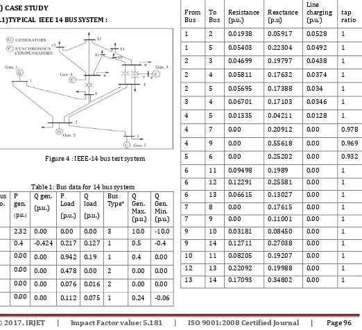
[image:4.595.42.564.321.797.2]3.1)TYPICAL IEEE 14 BUS SYSTEM :
Figure 4 : IEEE-14 bus test system
Table 1: Bus data for 14 bus system Bus
no. P gen.
(p.u.)
Q gen. (p.u.)
P Load (p.u.)
Q load (p.u.)
Bus
Type* Q Gen. Max. (p.u.)
Q Gen. Min. (p.u.) 1 2.32 0.00 0.00 0.00 3 10.0 -10.0 2 0.4 -0.424 0.217 0.127 1 0.5 -0.4 3 0.00 0.00 0.942 0.19 1 0.4 0.00
4 0.00 0.00 0.478 0.00 2 0.00 0.00 5 0.00 0.00 0.076 0.016 2 0.00 0.00 6 0.00 0.00 0.112 0.075 1 0.24 -0.06
7 0.00 0.00 0.00 0.00 2 0.00 0.00
8 0.00 0.00 0.00 0.00 1 0.24 -0.06 9 0.00 0.00 0.295 0.166 2 0.00 0.00
10 0.00 0.00 0.090 0.058 2 0.00 0.00
11 0.00 0.00 0.035 0.018 2 0.00 0.00 12 0.00 0.00 0.061 0.016 2 0.00 0.00 13 0.00 0.00 0.135 0.058 2 0.00 0.00
14 0.00 0.00 0.149 0.050 2 0.00 0.00 *Bus Type: (3) swing bus, (1) generator bus (PV bus), and (2) load bus (PQ bus)
Table 2 : Line data for 14 bus system
From
Bus To Bus Resistance (p.u.) Reactance (p.u) Line charging
(p.u.) tap ratio
1 2 0.01938 0.05917 0.0528 1
1 5 0.05403 0.22304 0.0492 1
2 3 0.04699 0.19797 0.0438 1
2 4 0.05811 0.17632 0.0374 1
2 5 0.05695 0.17388 0.034 1
3 4 0.06701 0.17103 0.0346 1
4 5 0.01335 0.04211 0.0128 1
4 7 0.00 0.20912 0.00 0.978
4 9 0.00 0.55618 0.00 0.969
5 6 0.00 0.25202 0.00 0.932
6 11 0.09498 0.1989 0.00 1
6 12 0.12291 0.25581 0.00 1
6 13 0.06615 0.13027 0.00 1
7 8 0.00 0.17615 0.00 1
7 9 0.00 0.11001 0.00 1
9 10 0.03181 0.08450 0.00 1
9 14 0.12711 0.27038 0.00 1
10 11 0.08205 0.19207 0.00 1
12 13 0.22092 0.19988 0.00 1
© 2017, IRJET | Impact Factor value: 5.181 | ISO 9001:2008 Certified Journal | Page 97
3.2) TYPICAL 5 BUS SYSTEM : [image:5.595.319.545.129.552.2]Figure 5: 5 bus system
Table 3: Bus data for 5 bus system
Bus PL QL PG QG V Bus
type
1 - - - - 1.02 slack
2 0 0 2 - 1.02 PV
3 0.5 0.2 0 0 - PQ
4 0.5 0.2 0 0 - PQ
5 0.5 0.2 0 0 - PQ
Line Data for 5 Bus system: Line impedances as per fig. 5 = 0.05+0.15i, Q2,min= 0.2 and Q2,max= 0.6
4) RESULTS AND DISCUSSIONS
[image:5.595.214.535.130.765.2]5- bus test system results
Table 4 : Bus load flow results for 5 bus system Bus
no. Bus type Voltage P Q
1 3 1.02 - -
2 1 4.2099+9.1756i 2 0.2448 3 2 -0.0191-3.243i -0.5 -0.2
4 2 0.4504 -0.5 -0.2
5 2 0.2154-3.8506i -0.5 -0.2
Table 5 : Line flow results for 5 bus system Fro
m Bus
To Bu s
Y P flow Q flow Line losses
1 2 2-6i 1.2204 0.7055 3.8199 1 5 2-6i -0.5498 -0.2453 0.6968 2 3 2-6i 3.0963 -16.8 7.2077 2 5 2-6i 3.1614 -17.4484 7.7618 3 4 2-6i 0.7074 -1.5959 0.5475 4 5 2-6i -0.1801 -0.0574 0.705
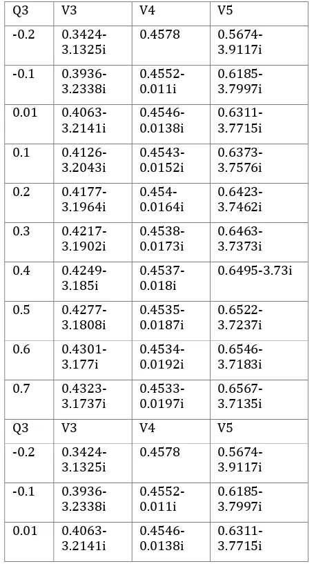
Table 6 : Effect of Q on Load bus voltages for 5 bus system
Q3 V3 V4 V5
-0.2
0.3424-3.1325i 0.4578 0.5674-3.9117i -0.1
0.3936-3.2338i 0.4552-0.011i 0.6185-3.7997i 0.01
0.4063-3.2141i 0.4546-0.0138i 0.6311-3.7715i 0.1
0.4126-3.2043i 0.4543-0.0152i 0.6373-3.7576i 0.2
0.4177-3.1964i 0.454-0.0164i 0.6423-3.7462i 0.3
0.4217-3.1902i 0.4538-0.0173i 0.6463-3.7373i 0.4
0.4249-3.185i 0.4537-0.018i 0.6495-3.73i 0.5
0.4277-3.1808i 0.4535-0.0187i 0.6522-3.7237i 0.6
0.4301-3.177i 0.4534-0.0192i 0.6546-3.7183i 0.7
0.4323-3.1737i 0.4533-0.0197i 0.6567-3.7135i
Q3 V3 V4 V5
-0.2
0.3424-3.1325i 0.4578 0.5674-3.9117i -0.1
0.3936-3.2338i 0.4552-0.011i 0.6185-3.7997i 0.01
0.4063-3.2141i 0.4546-0.0138i 0.6311-3.7715i
[image:5.595.63.296.159.368.2]© 2017, IRJET | Impact Factor value: 5.181 | ISO 9001:2008 Certified Journal | Page 98
IEEE-14 bus test system resultsTable 7 : Bus load flow results for 14 bus system Bus
no. Bus type Voltage P Q
1 3 1.06 - -
2 1 0.1978+4.0226i 0.4 0.4205
3 1 1.0841+0.3310i 0 -0.1178
4 2 -3.3406-4.8576i -0.478 0 5 2 9.8508+1.8584i -0.076 -0.016
6 1 -9.522-0.3288i 0 1.2988
7 2 4.9139+1.489i 0 0
8 1 -0.5687 0 .5569
[image:6.595.59.556.431.792.2]9 2 -2.1155-1.4875i -0.295 -.166 10 2 1.0398+0.4864i -0.09 -0.058 11 2 3.8424-0.0272i -0.035 0.018 12 2 2.5132-0.0063i -0.061 -0.016 13 2 5.11-0.4821i -0.135 -0.058 14 2 0.7776+0.0723i -0.149 -0.05
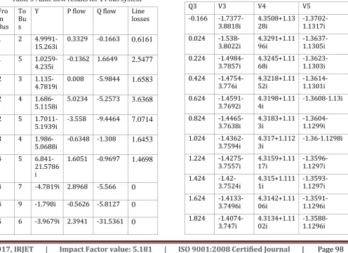
Table 5 : Line flow results for 14 bus system Fro
m Bus
To Bu s
Y P flow Q flow Line
losses
1 2
4.9991-15.263i 0.3329 -0.1663
0.6161
1 51.0259-4.235i -0.1362 1.6649
2.5477
2 31.135-4.7819i 0.008 -5.9844
1.6583
2 41.686-5.1158i 5.0234 -5.2573
3.6368
2 51.7011-5.1939i -3.558 -9.4464
7.0714
3 41.986-5.0688i -0.6348 -1.308
1.6453
4 56.841-21.5786 i
1.6051 -0.9697
1.4698
4 7 -4.7819i 2.8968 -5.566
0
4 9 -1.798i -0.5626 -5.8127
0
5 6 -3.9679i 2.3941 -31.5361
0
6 11
1.955-4.094i 8.774 -18.042
12.346
6
6 12
1.526-3.176i 10.2616 -21.0482
13.128
6
6 13
3.0989-6.1028i 7.0874 -12.7315
10.323
8
7 8 -5.677i 0.1152 -3.6169 0 7 9 -9.0901i -0.4811 2.4976 0 9 10
3.902-10.3654 i
0.16 -0.2664 0.1712
9 14
1.424-3.0294i 0.6083 -0.6688 0.5288 10 11
1.8809-4.4029i -0.4719 0.1962 0.6049 12 13
2.4785-2.1632i -1.3333 0.8195 1.0971 13 14
1.137-2.315i 3.2145 -5.8248 2.4574
Table 6 : Effect of Q on Load bus voltages for 14 bus system
Q3 V3 V4 V5
-0.166
-1.7377-3.8818i 4.3508+1.1328i -1.3702-1.1317i 0.024
-1.538-3.8022i 4.3291+1.1196i -1.3637-1.1305i 0.224
-1.4984-3.7857i 4.3245+1.1168i -1.3623-1.1303i 0.424
-1.4754-3.776i 4.3218+1.1152i -1.3614-1.1301i 0.624
-1.4591-3.7692i 4.3198+1.114i -1.3608-1.13i 0.824
-1.4465-3.7638i 4.3183+1.113i -1.3604-1.1299i 1.024
-1.4362-3.7594i 4.317+1.1123i -1.36-1.1298i 1.224
-1.4275-3.7557i 4.3159+1.1117i -1.3596-1.1297i 1.424
-1.42-3.7524i 4.315+1.1111i -1.3593-1.1297i 1.624
-1.4133-3.7496i 4.3142+1.1106i -1.3591-1.1296i 1.824
© 2017, IRJET | Impact Factor value: 5.181 | ISO 9001:2008 Certified Journal | Page 99
Figure 7 : V-Q curves and P-V curves for load bus 9For a 5 bus and IEEE 14 bus system system, after performing the load flow analysis using Newton Raphson method, the following points can be inferred from the P-V curves and V-Q curves :
If reactive power is injected into a load bus using reactive power compensation methods, the power factor of the load bus increases.
The P-V curve drawn at a constant power factor shifts to a higher power factor value on injection of the reactive power at the bus.
Voltage stability is improved if reactive power is injected into the load bus as due to increase in power factor, higher values of voltages can be obtained at same active power at the bus.
In the curve obtained, the voltage become constant at higher values of active power and thus the voltage stability decreases but the system does not tend towards the condition of voltage collapse and hence differs from the real time systems as the system under consideration is a standard system taking theoretical values of different parameters at buses.
Load shedding is another method for improving voltage stability as the active power at the load bus decreases thus improving the voltage.
In the V-Q curves obtained, system is unstable to the left of the knee point of the curve as the voltage decreases with increase in reactive power, but to the right of the knee point, the voltage increases with increase in reactive power and hence the system is stable for these values.
5) CONCLUSIONS AND FUTURE WORK
By utilizing the curves obtained at different power factors in P-V curves and at different values of active power in V-Q curve at each of the substation being monitored and obtaining the values of different parameters in real time, we can define a definite instability margin.
If the real time system enters into this instability margin, then we can take pre-emptive action against the problem by alarming the operator to inject the reactive power at the bus.
In case amount of reactive power compensation is less than required, then after applying all the compensation we can go for load shedding in such a way that voltage stability can be improved.
If the values of different parameters can be obtained continuously using new technologically advanced tools like SCADA, then we can also handle Dynamic Voltage Stability.
REFERENCES
[1]. C.W. Taylor. Power System Voltage Stability. McGrawHill, New York, 1994.
[2]. V. Borozan, M.E. Baran and D. Novosel, “Integrated Volt/Var Control in Distribution Systems”, in Proc. of IEEE Power Engineering Society Winter Meeting, 2001.
[3]. ChakrabartiA, Kothari D P and Mukhopadhyay , Performance, Operation and control of EHV Power Transmission Systems, I st ed, New Delhi Wheeler ch no 6 pp 132 -141. 2000.
[4]. Wadhawa C.L. Electrical Power System V ed New Age International (P) Limited Publishers, New Delhi.ch no 10 pp no 226-228 2009.
[5]. Mark N Nwohu “Voltage Stability Improvement using Static Var Compensator in Power Systems” Leonardo Journal of Sciences ISSN pp1583-0233., January – June 2009. [6]. “IEEE Recommended Practice for Excitation System Models for Power System Stability Studies‟‟, IEEE Power Engineering Society, New York, April 2006.
[7]. K. Vu: “Use of local measurements to estimate voltage stability margin‟‟, in IEEE Transaction on Power System, Vol. 14, No. 3, August 1999, p. 1029-123
[8]. Berger, A.R.; Vittal, Vijay; Power System Analysis; Pearson Education; 2005.
[9]. Ray, S.; Electrical Power Systems; Prentice-Hall-India ; 2007