Mathematical Models to Simultaneously Determine Overtime Requirements and Schedule Cells

(1)

http://dx.doi.org/10.4236/eng.2015.72006

Mathematical Models to Simultaneously

Determine Overtime Requirements and

Schedule Cells

Gürsel A. Süer, Kush Mathur

ISE Department, Ohio University, Athens, OH, USA Email: [email protected], [email protected]

Received 22 January 2015; accepted 10 February 2015; published 13 February 2015

This work is licensed under the Creative Commons Attribution International License (CC BY). http://creativecommons.org/licenses/by/4.0/

Abstract

The problem studied in this paper was inspired from an actual textile company. The problem is more complex than usual scheduling problems in that we compute overtime requirements and make scheduling decisions simultaneously. Since having tardy jobs is not desirable, we allow overtime to minimize the number of tardy jobs. The overall objective is to maximize profits. We present various mathematical models to solve this problem. Each mathematical model reflects different overtime workforce hiring practices. An experimentation has been carried out using eight different data sets from the samples of real data collected in the above mentioned textile company. Mathematical Model 2 was the best mathematical model with respect to both profit and execution time. This model considered partial overtime periods and also allowed different over-time periods on cells. We could solve problems up to 90 jobs per period. This was much more than what the mentioned textile company had to handle on a weekly basis. As a result, these models can be used to make these decisions in many industrial settings.

Keywords

Overtime Decisions, Cell Loading, Cell Scheduling, Mathematical Modeling

1. Introduction

(2)

overtime will be done or not, etc. Various approaches have been developed for capacity planning purposes such as capacity bills, resources profiles, rate-based capacity planning, and mathematical modeling, etc. On the other hand, scheduling deals with the detailed allocation of resources established in the capacity planning step to var-ious jobs over a period of time. Scheduling establishes start and completion times of jobs on resources, i.e. ma-chines, cells, production lines and workers.

In a company, each on-time delivered product brings revenue and customer satisfaction; both are essential to maintain the profitability of any company over a long term period. Making a job tardy is highly undesirable for any company. Establishing capacity requirements is a difficult task and it gets even harder when capacity re-quirements vary from one period to the next. In this situation, using overtime is a feasible method and many companies use that. Therefore, overtime can be used to adjust the capacity to handle the jobs which otherwise become tardy and may lead to poor reputation or in worst case loosing up of valuable customers. Overtimes are of two types: weekend overtime and weekday overtime. This distinction is important in that their costs usually vary. Weekend overtimes are usually more expensive than the weekday overtime because of the change in hourly workforce rate. Therefore, each overtime decision comes with a cost associated with it. This all makes the problem difficult to solve and lead to a NP-hard optimization problem where the weekend and weekday overtime decisions as well as cell loading and job sequencing are performed to maximize the overall net profit. We need to mention that if overtime is needed week after week, this may be an indicator that organization needs to re-assess capacity requirements and adjust regular capacity levels, i.e., increase number of cells, number of machines, etc.

2. Problem Definition

The problem studied in this paper was inspired from an actual textile company. In every planning period (week) there are n jobs to complete using m number of identical cells. Manufacturing cells are popular in the manufac-turing world. Cellular Manufacmanufac-turing (CM) aims to obtain the flexibility to produce a high or moderate variety of low or moderate demand products with high productivity. CM is a type of manufacturing system that consists of manufacturing cell(s) with dissimilar machines needed to produce part family/families. Generally, the prod-ucts grouped together form a product family. The benefits of CM are lower setup times, smaller lot sizes, lower work-in-process inventory and less space, reduced material handling, and shorter flow time, simpler work flow (Suresh & Kay, 1998 [1]). Cellular Manufacturing also simplifies planning and control of various tasks floating on the shop floor. Cells are ideally equipped with all of the machines needed to produce a productor product family (independent) and usually follow uni-directional flow (flowshop).

Many textile companies also use cells to enjoy the benefits the cells have to offer. Machines used in cells in textile industry are usually limited to different types of sewing machines such as overlock machines, stitch ma-chines, automatic flat lock sewing machines. In this study, each cell can perform eight operations. The tions performed are briefly discussed in this paragraph. The first operation is cutting and the next three opera-tions require sewing machines. The operaopera-tions that follow are finishing, ironing, cleaning and packing. Opera-tions 2 and 4 each were performed on two identical machines as they were the slowest operaOpera-tions. It is easy to re-configure cells in the textile industry once products with different requirements are produced as machines and work benches are easier to move around.

In this paper, it is assumed that each job has its own individual due date. The modeling gets complicated in that we need to decide additional capacity requirements at the same time we make scheduling decisions. Any job that cannot be completed by its due date becomes tardy and is assumed lost sales. Having tardy jobs is not de-sirable as this adversely affects relationships with customers and thus reputation of the firm in the long term. As a result, we allow overtime to minimize the number of tardy jobs. Overtime decisions are made for shifts on a daily basis. Overtime can be done during the weekends (Saturday and Sunday) as well as weekdays. Weekend overtime is done prior to upcoming week. It is also assumed that weekend overtime cost is higher than weekday overtime cost. The overall objective is to maximize profits. Tardy jobs are avoided as long as profit to be made is higher than the corresponding production/overtime costs. There are limitations on weekday and weekend overtime capacities. In this paper, the number of shifts considered is 2. Models can easily be modified to ac-commodate 1 shift. However, if the company wants to adopt a 3-shift policy, then weekday overtime option has to be eliminated and overtime can only be done during weekends. Lot splitting is not allowed in this study.

(3)

3. Literature Review

Several researchers focused on cell loading problem. Among them, Süer, Saiz, Dagli & Gonzalez [2] andSuer, Saiz & Gonzalez [3] developed several simple cell loading rules for connected and independent cells, respec-tively. They have tested the performance of these rules against four different performance measures, namely number of tardy jobs, maximum tardiness, total tardiness and utilization. Süer, Vazquez & Cortes [4] developed a hybrid approach of Genetic Algorithms (GA) and local optimizer to minimize number of tardy jobs in a mul-ti-cell environment. In the same study, they have used three different GA approaches; basic GA approach, hybr-id GA with local optimizers and finally GA with learning feature. Hybrhybr-id GA outperformed basic GA, however, GA with learning improved solutions only marginally. Süer, Arikan & Babayiğit [5] [6] studied cell loading subject to manpower restrictions and developed fuzzy mathematical models to minimize number of tardy jobs and total manpower levels. They have used various fuzzy operators and identified fuzzy operators that can find non-dominated solutions. In their work, number of cells and crew size for each cell were identified in addition to product sequencing decisions.

There are a number of works reported where both cell loading and product sequencing tasks are carried out. Süer & Dagli [7] and Süer, Cosner & Patten [8] discussed models to minimize makespan, machine requirements and manpower transfers. These works first assigned products to cells to minimize makespan and then re-se- quenced the products to minimize manpower requirements. Yarimoglu [9] developed a mathematical model and a genetic algorithm to minimize manpower shortages in cells with synchronized material flow. Synchronized material flow allowed material transfers between stages at regular intervals (e.g., 4 hour in his case).

Some other researchers studied the sequencing of families in a single cell or machine. Nakamura, Yoshida & Hitomi [10] considered sequence-independent group setup in his work and his objective was to minimize total tardiness. Hitomi & Ham [11] also considered sequence-independent setup times for a single machine schedul-ing problem. Ham, Hitomi, Nakamura & Yoshida [12] developed a branch-and-bound algorithm for the optimal group and job sequence to minimize total flow time keeping the number of tardy jobs minimum. Pan and Wu [13] focused on single machine scheduling problem to minimize mean flow time of all jobs subject to due date satisfaction. They categorized the jobs into groups without family splitting. Gupta and Chantaravarapan [14] studied the single machine scheduling problem to minimize total tardiness considering group technology. Indi-vidual due dates and independent family setup times have been used in their problem with no family splitting. Süer and Mese [15] studied the same problem but allowed family splitting as it would be beneficial in many cases.

A number of researchers focused on shoe manufacturing industry and reported various results. These works heavily focused on scheduling jobs on the Rotary Injection Molding Machines. Süer. Santos and Vazquez [16] have developed a three-phase Heuristic Procedure to minimize makespan. Süer, Subramanian and Huang [17] included some heuristic procedures and mathematical models for cell loading and scheduling problem. The ob-jective was to minimize makespan and unlimited availability of the molds was assumed. Later, Huang, Suer and Urs [18] introduced the limited mold availability into the problem for the same objective.

The most important feature of the scheduling problem studied in this paper is that both overtime decisions and detailed scheduling tasks including cell loading and product sequencing are performed simultaneously. Even though there were previous works that considered capacity and scheduling decisions simultaneously before (see Süer, Arikan & Babayiğit [5] [6]), there is only one work that considers both overtime and scheduling decisions simultaneously (see Mathur and Süer [19]) in the literature to the best knowledge of the authors. We propose new mathematical models that can be used under varying conditions. The objective is to maximize the profit and it is closely related to finishing jobs on time.

4. Integer Programming Formulation

(4)

formula-tion is that the due time for a job is extended (increased) by the total overtime hours planned before this job is due.

Assume that a job is due Wednesday noon. Assuming only one shift work, then the due time for this job is calculated as 20 hours (8 hours available on Monday, 8 hours available on Tuesday and 4 hours available on Wednesday). Assume that mathematical model proposes to do overtime both on Monday and Tuesday, 3 hours each day. Then the due time of this job becomes 26 hours (=20 + 3 + 3). The proposed mathematical models accommodate this possibility in the formulation. The objective is to maximize profit. All of the jobs should be ordered by the Earliest Due Date (EDD) before model is run (d[1] ≤ d[2]≤ d[3]≤ … ≤ d[n]). Similarly p[i] is the

processing time of the job in the ith order. It is also assumed that weekend overtime work is done prior to plan-ning week.

In this section, four different integer programming formulations are introduced. Each one of them is based on the observation on overtime workforce handling practices followed by the industries. Indices and parameters used throughout the paper are listed below.

Indices: i: job index j: cell index t: day index q: shift index Parameters: n: number of jobs

m: number of identical cells pi: processing time of job i (in hours)

di: due time of job i (in hours)

shift[i]v:shift in which ith job is due

si: sales price of job i

cwd: weekday overtime cost per shift cwe: weekend overtime cost per shift dayi: due day of job i depending on due time

otwd: length of weekday overtime (3 hours) otwe: length of weekend overtime (8 hours)

4.1. Mathematical Model 1

The unique feature about this model is that it allows different weekday and weekend overtime decisions with respect to different cells and also workers are paid for the complete period of overtime slot even if they finish the work early in the overtime period. The model is capable of determining the schedule of jobs on each cell as well as handling the capacity of each cell by making overtime decisions.

The objective is to maximize the net profit as shown in Equation (1). This is computed by subtracting all weekend and weekday overtime costs from the sales revenue of the products finished by their due time. Week-day overtime can be done on any of the five working Week-days and weekend overtime can be done on SaturWeek-day and/or Sunday. The first set of constraints (Equation (2)) enforce that early jobs are completed before their due times (original or extended). The second set of constraints (Equation (3)) guarantees that a job can assigned to at most one cell. The values of decision variables xijand ottjq will be known once the mathematical model is solved.

Decision Variables:

xij: 1 if job i is assigned to cell j, 0 otherwise

ottjq: 1 if there is overtime on day t in shift q of cell j, 0 otherwise

Objective Function:

5 2 7 2

1 1 1 1 1 6 1 1

Max

n m m m

i ij tjq tjq

i j t j q t j q

z s x cwd ot cwe ot

= = = = = = = =

=

_∑∑

−

_∑∑∑

−

_∑∑∑

(1)

Subject to:

[ ] [ ] [ ]

[ ] [ ]

day shift 7 2

1 1 1 6 1

1, 2, , , 1, 2, ,

k k

k

tjq tjq

i i j k

i t q t q

p x d otwd ot otwe ot k n j m

= = = = =

≤ + + ∀ = ∀ =

(5)

1

1 1, 2,

m

ij j

x i n

=

≤ ∀ =

∑

 (3)

4.2. Mathematical Model 2

Model 2 is similar to Model 1 in that it allows different weekday and weekend overtime work with respect to different cells. However, the difference between two models comes from the practice that overtime workforces can be hired and paid for the fraction of the overtime slot in this Model. In this model, overtime decision varia-ble is modified as given below.

ottjq: fraction of overtime to do on day t in shift q of cell j between 0 and 1

4.3. Mathematical Model 3

The model has been first proposed by Süer, Mathur and Ji [19]. The unique feature about this model is that a uniform overtime strategy is applied, i.e., all of the cells get to do the same overtime whenever an overtime de-cision is made. This may be important in some companies where all the workers are given the same opportunity to do overtime and gain additional income. Overtime workforces are hired and paid for the complete period of overtime slot on all cells. In this case, overtime decision variable is simplified as shown below.

ottq: 1 if there is overtime on day t in shift q, 0 otherwise

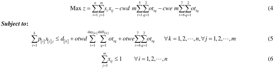
The objective is to maximize the net profit as shown in Equation (4). The first set of constraints (Equation (5)) enforce that early jobs are completed before their due times (original or extended). The second set of constraints (Equation (6)) guarantees that a job can assigned to at most one cell.

Objective Function:

5 2 7 2

1 1 1 1 6 1

Max

n m

i ij tq tq

i j t q t q

z s x cwd m ot cwe m ot

= = = = = =

=

_∑∑

−

_∑∑

−

_∑∑

(4)

Subject to:

[ ] [ ] [ ]

[ ] [ ]

day shift 7 2

1 1 1 6 1

1, 2, , , 1, 2, ,

k k

k

tq tq

i i j k

i t q t q

p x d otwd ot otwe ot k n j m

= = = = =

≤ + + ∀ = ∀ =

∑

∑ ∑

∑∑

  (5)

1

1 1, 2, ,

m

ij j

x i n

=

≤ ∀ =

∑

 (6)

4.4. Mathematical Model 4

Model 4 is similar to Model 3 in that all of the cells get to do the same overtime whenever an overtime decision is made. However, the difference between two models is that overtime workforces can be hired and paid for the fraction of the overtime slot in Model 4. In this case, overtime decision variable is modified as shown below.

ottq: fraction of overtime to do on day t in shift q between 0 and 1

The main features of four mathematical models are summarized inTable 1.

5. A Numerical Illustration

[image:5.595.95.535.356.475.2]

An example case is illustrated in this section. A 20-job and 2-cell problem is solved by all four mathematical models using ILOG OPL 6.3 optimization tool. In each mathematical model illustration, three tables and one figure are given. The first table shows the sequence of jobs assigned to each cell; the second table shows the corresponding overtime decisions for the problem; the third table shows the original due day, due shift and due time; revenue generated from each job, processing times, detailed computations of completion times and revised due dates (Di*) based on overtime decisions; and the Gantt chart is given in the corresponding figure. It is

im-portant to note that the weekend overtime starts before the week starts. For example, to complete a job before the set due date (say on Monday evening), overtime can be performed on Saturday and/or Sunday shifts.

5.1. Solution by Mathematical Model 1

(6)

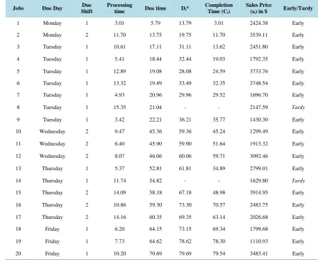
paper lost customer orders). The jobs assigned to each cell are summarized inTable 2.Table 3 shows when and on what cell we need to do overtime during the week.Table 4 shows the details of all computations. When a job is tardy, its completion time is not listed since it is assumed as lost sales (for example for job 8 inTable 4). Job 1 inTable 4 is due Monday, shift 1, and original due time is 5.79 hours and it has been assigned to cell 1. Since we allow overtime on Sunday shift 1 for eight hours on cell 1, the due date is taken as (D1*=) 13.79 hours (=5.79

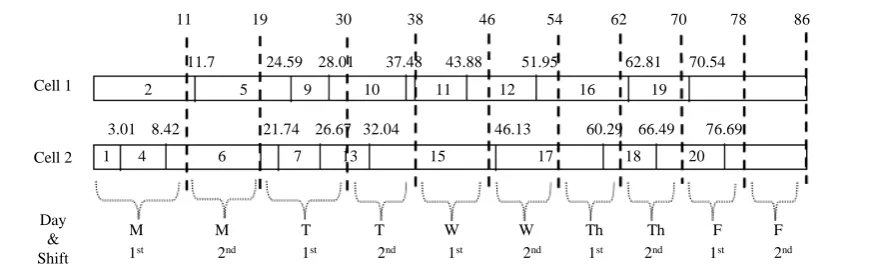
+ 8). Similar adjustment are made for all jobs, i.e. jobs original due dates are modified (increased) by consider-ing the overtimes scheduled before their due date. On cell 1, Monday shift1 is of regular eight hours whereas on cell 2, Monday shift 1 is of 11 hours (including overtime). On both the cells, Monday shift 2 are 11 hours (in-cluding overtimes); Tuesday shift 1 and shift 2 are 11 (in(in-cluding overtimes) and eight hours respectively; and the remaining weekdays are all regular eight hours. Whereas on the weekends, only cell 1 needs eight hours of overtime only on Sunday shift1 as shown inTable 3 andFigure 1.

Table 1. Characteristics of Mathematical models over Overtime decision variables.

Mathematical Models Overtime

Different on different cells Same on all cells Complete duration Partial duration

Mathematical Model 1  

Table 2. Sequence of jobs assigned to each cell for model 1.

Cells Jobs

C1 1, 3, 4, 6, 9, 10, 11, 12, 16, 19

C2 2, 5, 7, 13, 15, 17, 18, 20

Table 3. Overtime decisions for model 1.

Day Monday Tuesday Wednesday Thursday Friday Saturday Sunday

Cells

C1 Shift 1 0 1 0 0 0 0 1

Shift 2 1 0 0 0 0 0 0

C2 Shift 1 1 1 0 0 0 0 0

Shift 2 1 0 0 0 0 0 0

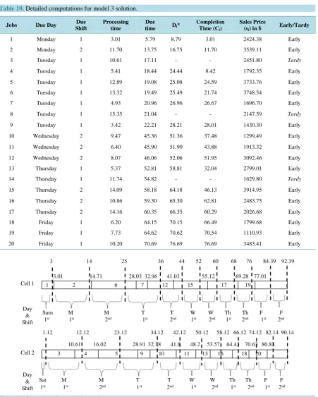
Figure 1. Gantt chart for model 1 solution.

8 16 27 38 46 54 62 70 78 86 94

3.01 13.62 19.03 32.35 35.77 45.24 51.64 59.71 70.57 78.3

1 3 4 6 9 10 11 12 16 19

Sum M M T T W W Th Th F F 1st ₁st ₂nd ₁st ₂nd ₁st ₂nd ₁st ₂nd ₁st ₂nd

11 22 33 41 49 57 65 73 81 89

11.7 24.59 29.52 34.89 48.98 63.14 69.34 79.54 2 5 7 13 15 17 18 20

M M T T W W Th Th F F 1st ₂nd ₁st ₂nd ₁st ₂nd ₁st ₂nd ₁st ₂nd Cell 1

Day & Shift

Cell 2

(7)

[image:7.595.80.539.103.480.2]

Table 4. Detailed computations for model 1 solution.

Jobs Due Day Due

Shift

Processing

time Due time Di*

Completion Time (Ci)

Sales Price

(si) in $ Early/Tardy

1 Monday 1 3.01 5.79 13.79 3.01 2424.38 Early

2 Monday 2 11.70 13.75 19.75 11.70 3539.11 Early

3 Tuesday 1 10.61 17.11 31.11 13.62 2451.80 Early

4 Tuesday 1 5.41 18.44 32.44 19.03 1792.35 Early

5 Tuesday 1 12.89 19.08 28.08 24.59 3733.76 Early

6 Tuesday 1 13.32 19.49 33.49 32.35 3748.54 Early

7 Tuesday 1 4.93 20.96 29.96 29.52 1696.70 Early

8 Tuesday 1 15.35 21.04 - - 2147.59 Tardy

9 Tuesday 1 3.42 22.21 36.21 35.77 1430.30 Early

10 Wednesday 2 9.47 45.36 59.36 45.24 1299.49 Early

11 Wednesday 2 6.40 45.90 59.90 51.64 1913.32 Early

12 Wednesday 2 8.07 46.06 60.06 59.71 3092.46 Early

13 Thursday 1 5.37 52.81 61.81 34.89 2799.01 Early

14 Thursday 1 11.74 54.82 - - 1629.80 Tardy

15 Thursday 2 14.09 58.18 67.18 48.98 3914.95 Early

16 Thursday 2 10.86 59.30 73.30 70.57 2483.75 Early

17 Thursday 2 14.16 60.35 69.35 63.14 2026.68 Early

18 Friday 1 6.20 64.15 73.15 69.34 1799.68 Early

19 Friday 1 7.73 64.62 78.62 78.30 1110.93 Early

20 Friday 1 10.20 70.69 79.69 79.54 3483.41 Early

5.2. Solution by Mathematical Model 2

This model also assigned 18 out of 20 jobs to cells as shown inTable 5. On both cells, Monday shifts are 11 hours (including overtimes); Tuesday shift1 and shift 2 are 11 (including overtimes) and 8 hours, respectively; and the remaining weekdays except for Friday shift 1 are all regular eight hours. On cell 1, Friday shift 1 is of 8.39 hours (=8 + 0.13*3) whereas on cell 2 it is of 8.02 hours (=8 + 0.0067*3) including overtimes. On the weekends, overtimes are required on Sunday shift 1 of 3 hours (=0.375*8) on cell 1 and on Saturday shift 1 of 1.12 hours (=0.14*8) on cell 2 as shown inTable 6. In this case, the due date for job 1 (D1*=) is computed as

11.79 hours since we allow partial overtime on Sunday shift 1 for three hours (=0.375*8) and also allow three hour overtime on shift1 on Monday on cell 1 (=5.79 + 3 + 3).Table 7 shows the details of all computations and the corresponding Gantt chart is given inFigure 2.

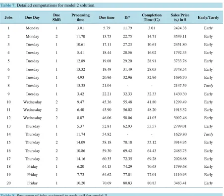
5.3. Solution by Mathematical Model 3

This model resulted in three tardy jobs. The sequence of jobs assigned to cells is given inTable 8. Overtime de-cisions are summarized in Table 9. On both the cells, Monday as well as Tuesday shift 1 and shift 2 are of 11 hours (including overtimes) and eight hours respectively; and the remaining days are all regular eight hours. On the other hand, no overtime work is scheduled for weekends. In this model, the due date for job 1 (D1*=) is

(8)

Cells Jobs

C1 1, 2, 6, 7, 12, 15, 17, 19

C2 3, 4, 5, 9, 10, 11, 13, 16, 18, 20

Cells C1

Shift 1 1 1 0 0 0.13 0 0.375

Shift 2 1 0 0 0 0 0 0

C2 Shift 1 1 1 0 0 0.0067 0.14 0

[image:8.595.88.541.264.660.2]

Shift 2 1 0 0 0 0 0 0

Shift

Processing

time Due time Di*

Sales Price

1 Monday 1 3.01 5.79 11.79 3.01 2424.38 Early

2 Monday 2 11.70 13.75 22.75 14.71 3539.11 Early

3 Tuesday 1 10.61 17.11 27.23 10.61 2451.80 Early

4 Tuesday 1 5.41 18.44 28.56 16.02 1792.35 Early

5 Tuesday 1 12.89 19.08 29.20 28.91 3733.76 Early

6 Tuesday 1 13.32 19.49 31.49 28.03 3748.54 Early

7 Tuesday 1 4.93 20.96 32.96 32.96 1696.70 Early

8 Tuesday 1 15.35 21.04 - - 2147.59 Tardy

9 Tuesday 1 3.42 22.21 32.33 32.33 1430.30 Early

10 Wednesday 2 9.47 45.36 55.48 41.80 1299.49 Early

11 Wednesday 2 6.40 45.90 56.02 48.20 1913.32 Early

12 Wednesday 2 8.07 46.06 58.06 41.03 3092.46 Early

13 Thursday 1 5.37 52.81 62.93 53.57 2799.01 Early

14 Thursday 1 11.74 54.82 - - 1629.80 Tardy

15 Thursday 2 14.09 58.18 70.18 55.12 3914.95 Early

16 Thursday 2 10.86 59.30 69.42 64.43 2483.75 Early

17 Thursday 2 14.16 60.35 72.35 69.28 2026.68 Early

18 Friday 1 6.20 64.15 74.29 70.63 1799.68 Early

19 Friday 1 7.73 64.62 77.01 77.01 1110.93 Early

20 Friday 1 10.20 70.69 80.83 80.83 3483.41 Early

Cells Jobs

C1 2, 5, 9, 10, 11, 12, 16, 19

(9)

Shift 1 1 1 0 0 0 0 0

Shift 2 0 0 0 0 0 0 0

Shift

Processing time

Due

time Di*

Sales Price

1 Monday 1 3.01 5.79 8.79 3.01 2424.38 Early

2 Monday 2 11.70 13.75 16.75 11.70 3539.11 Early

3 Tuesday 1 10.61 17.11 - - 2451.80 Tardy

4 Tuesday 1 5.41 18.44 24.44 8.42 1792.35 Early

5 Tuesday 1 12.89 19.08 25.08 24.59 3733.76 Early

6 Tuesday 1 13.32 19.49 25.49 21.74 3748.54 Early

7 Tuesday 1 4.93 20.96 26.96 26.67 1696.70 Early

8 Tuesday 1 15.35 21.04 - - 2147.59 Tardy

9 Tuesday 1 3.42 22.21 28.21 28.01 1430.30 Early

10 Wednesday 2 9.47 45.36 51.36 37.48 1299.49 Early

11 Wednesday 2 6.40 45.90 51.90 43.88 1913.32 Early

12 Wednesday 2 8.07 46.06 52.06 51.95 3092.46 Early

13 Thursday 1 5.37 52.81 58.81 32.04 2799.01 Early

14 Thursday 1 11.74 54.82 - - 1629.80 Tardy

15 Thursday 2 14.09 58.18 64.18 46.13 3914.95 Early

16 Thursday 2 10.86 59.30 65.30 62.81 2483.75 Early

17 Thursday 2 14.16 60.35 66.35 60.29 2026.68 Early

18 Friday 1 6.20 64.15 70.15 66.49 1799.68 Early

19 Friday 1 7.73 64.62 70.62 70.54 1110.93 Early

[image:9.595.90.542.150.714.2]

20 Friday 1 10.20 70.69 76.69 76.69 3483.41 Early

3 14 25 36 44 52 60 68 76 84.39 92.39

Sum M M T T W W Th Th F F 1st ₁st ₂nd ₁st ₂nd ₁st ₂nd ₁st ₂nd ₁st ₂nd Cell 1

Day & Shift

Cell 2

Day & Shift

3.01 14.71 28.03 32.96 41.03 55.12 69.28 77.01

1 2 6 7 12 15 17 19

1.12 12.12 23.12 34.12 42.12 50.12 58.12 66.12 74.12 82.14 90.14

10.61 16.02 28.91 32.38 41.8 48.2 53.57 64.43 70.63 80.83

3 4 5 9 10 11 13 16 18 20

(10)

[image:10.595.102.538.80.216.2]

5.4. Solution by Mathematical Model 4

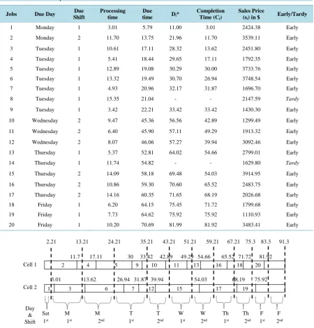
This model also led to 18 jobs being completed before their due dates. The sequence of jobs assigned to cells is given in Table 11. Overtime decisions are summarized in Table 12. InTable 13, for example Job 1, is due Monday, shift 1, and original due time is 5.79 hours. Since we allow partial overtime of 2.21 hours (=0.27625*8) on Saturday shift1 and also allow three hour overtime on Monday shift 1 on both the cells, the due date is taken as (D1*=) 11 hours (=5.79 + 2.21 + 3). Similar adjustment are made for all jobs, i.e. jobs original due dates are

modified (increased) by considering the overtimes scheduled before their due date. On both the cells, Monday shift 1 and shift 2 are 11 hours (including overtimes) each; Tuesday shift 1 and shift 2 are 11 hours (including overtimes) and regular of eight hours, respectively; Thursday shift 1 and shift 2 are regular eight hours and 8.09 hours (=8 + 0.03*3) (including overtime) respectively and the remaining days are all regular eight hours. Whe-reas on the weekend on both the cells, overtime is required only on Saturday shift 1 of 2.21 hours (=0.27625*8) as shown inFigure 4.

6. Experimentation Results

In this section, experimentation results are discussed. Eight problems were formed with 20, 30, 40, 50, 60, 70, 80 and 90 jobs; and 2, 2, 2, 2, 2, 4, 4 and 5 cells, respectively (problems 1, 2, 3, 4, 5, 6, 7 and 8 respectively). The data generated is inspired from the Textile Company where the problem was observed. Each product un-dergoes eight different operations. The upper and lower range of processing times for each operation were iden-tified based on the sample data provided by the company. The processing times were generated randomly from this interval for the corresponding operation in each data set. Processing times for operations 1, 2, 3, 4, 5, 6, 7 and 8 follow uniform distributions UD(2, 4), US(1, 2.5), UD(1, 3.5), UD(1, 2), UD(1, 2), UD(1, 2), UD(1, 2), and UD(0.2, 2), respectively. The batch size of each product follows uniform distribution UD(50, 250). The production rate for each product is identified based on the bottleneck machine. The processing time (hr) for a job is computed dividing its batch size with its production rate. The due time of each job is generated by using Equ-ation (7). Products’ due days (considering one week as a period) as well as a due shifts (1 or 2) are calculated on the basis of due time. The sale price of each job is assigned by using Equation (8). The hourly labor rates for regular time, weekday overtime and weekend overtime are taken as $10, $15, and $20, respectively. The week-end overtime is limited to 8 hours per shift whereas weekday overtime is restricted to 3 hours per shift.

(

)

1

1,10

n i i

i i

p

d p UD

n

=

 

 

= + ×

 

 

∑

₍₇₎

(

)

200 1 0.25, 0.5

i i

s =p × × +_ UD _ (8)

6.1. Results of Mathematical Model 1

The results of Mathematical Model1 are shown in Table 14. The results show that mathematical model pro-duced tardy jobs in spite of the fact that overtime was done both during the weekdays and weekend for some problems (problems 1, 4, and 5). In problems 2, 7, 8, weekend overtime was not done even though there was a

Cell 1

Cell 2

Day & Shift

11 19 30 38 46 54 62 70 78 86

M M T T W W Th Th F F 1st ₂nd ₁st ₂nd ₁st ₂nd ₁st ₂nd ₁st ₂nd

11.7 24.59 28.01 37.48 43.88 51.95 62.81 70.54

2 5 9 10 11 12 16 19

3.01 8.42 21.74 26.67 32.04 46.13 60.29 66.49 76.69

(11)

Cells Jobs

C1 2, 4, 5, 9, 10, 11, 13, 16, 18, 20

C2 1, 3, 6, 7, 12, 15, 17, 19

Shift 1 1 1 0 0 0 0.27625 0

[image:11.595.89.540.237.709.2]

Shift 2 1 0 0 0.03 0 0 0

Shift

Processing time

Due

time Di*

Sales Price

1 Monday 1 3.01 5.79 11.00 3.01 2424.38 Early

2 Monday 2 11.70 13.75 21.96 11.70 3539.11 Early

3 Tuesday 1 10.61 17.11 28.32 13.62 2451.80 Early

4 Tuesday 1 5.41 18.44 29.65 17.11 1792.35 Early

5 Tuesday 1 12.89 19.08 30.29 30.00 3733.76 Early

6 Tuesday 1 13.32 19.49 30.70 26.94 3748.54 Early

7 Tuesday 1 4.93 20.96 32.17 31.87 1696.70 Early

8 Tuesday 1 15.35 21.04 - - 2147.59 Tardy

9 Tuesday 1 3.42 22.21 33.42 33.42 1430.30 Early

10 Wednesday 2 9.47 45.36 56.56 42.89 1299.49 Early

11 Wednesday 2 6.40 45.90 57.11 49.29 1913.32 Early

12 Wednesday 2 8.07 46.06 57.27 39.94 3092.46 Early

13 Thursday 1 5.37 52.81 64.02 54.66 2799.01 Early

14 Thursday 1 11.74 54.82 - - 1629.80 Tardy

15 Thursday 2 14.09 58.18 69.48 54.03 3914.95 Early

16 Thursday 2 10.86 59.30 70.60 65.52 2483.75 Early

17 Thursday 2 14.16 60.35 71.65 68.19 2026.68 Early

18 Friday 1 6.20 64.15 75.45 71.72 1799.68 Early

19 Friday 1 7.73 64.62 75.92 75.92 1110.93 Early

20 Friday 1 10.20 70.69 81.99 81.92 3483.41 Early

Cell 1

Cell 2

Day & Shift

Sat M M T T W W Th Th F F 1st ₁st ₂nd ₁st ₂nd ₁st ₂nd ₁st ₂nd ₁st ₂nd

2.21 13.21 24.21 35.21 43.21 51.21 59.21 67.21 75.3 83.3 91.3

11.7 17.11 30 33.42 42.89 49.29 54.66 65.52 71.72 81.92 2 4 5 9 10 11 13 16 18 20

3.01 13.62 26.94 31.87 39.94 54.03 68.19 75.92

(12)

[image:12.595.87.540.101.243.2]

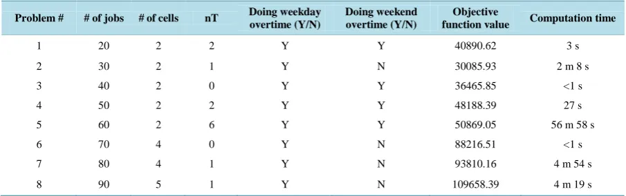
Table 14. Mathematical model 1 results.

Problem # # of jobs # of cells nT Doing weekday

overtime (Y/N)

Doing weekend overtime (Y/N)

Objective

function value Computation time

1 20 2 2 Y Y 40890.62 3 s

2 30 2 1 Y N 30085.93 2 m 8 s

3 40 2 0 Y Y 36465.85 <1 s

4 50 2 2 Y Y 48188.39 27 s

5 60 2 6 Y Y 50869.05 56 m 58 s

6 70 4 0 Y N 88216.51 <1 s

7 80 4 1 Y N 93810.16 4 m 54 s

8 90 5 1 Y N 109658.39 4 m 19 s

tardy job in the system. Doing overtime would cost more than profit to be obtained from this tardy in these problems. In problem 3, tardy job(s) were avoided by doing overtime both weekdays and weekends. Finally, in problem 6, weekday overtime was sufficient to avoid tardy jobs. The execution times of models varied from 1 second to almost 57 minutes.

6.2. Results of Mathematical Model 2

The results of Mathematical Model 2 are summarized inTable 15. There were tardy jobs in problems 1, 2, and 5 even though overtime was done both during the weekdays and weekend. In problems 3 and 4, tardy job(s) were avoided by doing overtime both weekdays and weekend. Finally, in problems 6, 7 and 8, weekday overtime was sufficient to avoid tardy jobs. The execution times of models were less than 2 seconds.

6.3. Results of Mathematical Model 3

The results of Mathematical Model 3 are given inTable 16. In problems 4 and 5, there were tardy jobs even though overtime was done both during the weekdays and weekend. In problems 1 and 2, weekend overtime was not done even though there were tardy jobs in the system. Finally, in problems 3, 6 and 8, tardy jobs were avoided by doing overtime either on weekdays or both weekdays and weekend. Problem 7 could not be solved due to memory restrictions. The execution times of models varied from 1 second to almost 2 hours 4 minutes.

6.4. Results of Mathematical Model 4

The results of Mathematical Model 4 are shown inTable 17. The results show that mathematical model pro-duced tardy jobs in spite of the fact that overtime was done both during the weekdays and weekend for some problems (problems 1, 4, and 5). In problems 2, 7, 8, weekend overtime was not done even though there was a tardy job in the system. Doing overtime would cost more than profit to be obtained from this tardy in these problems. In problem 3, tardy job(s) were avoided by doing overtime both weekdays and weekends. Finally, in problem 6, weekday overtime was sufficient to avoid tardy jobs. The execution times of models varied from 1 second to almost 57 minutes.

6.5. Comparison of Mathematical Models

(13)

overtime (Y/N)

Objective

function value Computation time 1 20 2 2 Y Y 41155.12 <1 s

2 30 2 1 Y Y 30243.78 <1 s

3 40 2 0 Y Y 36622.85 <1 s

4 50 2 0 Y Y 48557.07 <1 s

5 60 2 6 Y Y 50876.50 9 s

6 70 4 0 Y N 88311.01 <1 s

7 80 4 0 Y N 94068.04 2 s

8 90 5 0 Y N 109881.77 2 s

overtime (Y/N)

Objective

1 20 2 3 Y N 40488.82 <1 s

2 30 2 1 Y N 30081.08 4 m 24 s

3 40 2 0 Y Y 36465.85 <1 s

4 50 2 1 Y Y 48168.69 <1 s

5 60 2 6 Y Y 50869.05 2 h 3 m 31 s

6 70 4 0 Y N 88216.51 <1 s

7 80 4 out of memory

[image:13.595.90.544.59.754.2]

8 90 5 0 Y N 109632.80 <1 s

overtime (Y/N)

Objective

1 20 2 2 Y Y 41155.12 <1 s

2 30 2 1 Y Y 30243.78 <1 s

3 40 2 0 Y Y 36622.85 <1 s

4 50 2 0 Y Y 48557.07 <1 s

5 60 2 6 Y Y 50876.50 6 m 41 s

6 70 4 0 Y N 88311.01 3 m 27 s

7 80 4 0 Y Y 94068.04 17 s

[image:13.595.90.538.581.722.2]

8 90 5 0 Y N 109881.77 15 m 36 s

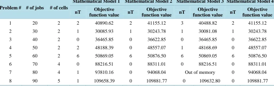
Table 18. Performance comparison between mathematical models.

Problem # # of jobs # of cells

Mathematical Model 1 Mathematical Model 2 Mathematical Model 3 Mathematical Model 4

nT Objective

function value nT

Objective function value nT

Objective function value

1 20 2 2 40890.62 2 41155.12 3 40488.82 2 41155.12

2 30 2 1 30085.93 1 30243.78 1 30081.08 1 30243.78

3 40 2 0 36465.85 0 36622.85 0 36465.85 0 36622.85

4 50 2 2 48188.39 0 48557.07 1 48168.69 0 48557.07

5 60 2 6 50869.05 6 50876.50 6 50869.05 6 50876.50

6 70 4 0 88216.51 0 88311.01 0 88216.51 0 88311.01

7 80 4 1 93810.16 0 94068.04 Out of memory 0 94068.04

(14)

7. Conclusions and Future Work

In this study, various mathematical models are proposed to determine overtime requirements, assign jobs to cells and also determine the sequence of jobs simultaneously in each cell. The objective is to maximize the profit to be obtained from the completion of products on time. These mathematical models represent different overtime workforce handling practices followed by industries. The problem has been inspired from a textile company. Data used in the experimentation has been generated based on the collected sample real data from the same company.

The result of a mathematical model gives us a weekly complete schedule with the overtime decisions on each weekend and weekday on each shift and on each cell. Moreover, it tells us the load on cells and also the sche-dule of jobs on each cell. The selection of an appropriate mathematical model obviously depends on practices of different companies. However, if there is a chance to select among these models, then Mathematical Model 2 would be the best choice as it outperforms all other mathematical models in all of the problems tested. Mathe-matical Model 2 allows partial overtime periods. It also allows different overtime periods on different cells. This flexibility in the problem formulation led to the best results. Mathematical model 4 tied the results in two of the problems and got the second best results in the rest of the problems. Indeed, the gap between the best and worst results when all models were considered was smaller than 1.62%.

The experimentation also showed that mathematical models could solve large problems relatively fast. Espe-cially Mathematical Model 2 took less than nine seconds to find the optimal solution in all of the problems tested. This may be another factor that would make Mathematical Model 2 a desirable one in addition to the fact that it found the highest profits among all models. We could solve problems up to 90 jobs per period. The num-ber of jobs mentioned in the textile company had to handle on a weekly basis roughly varied 20 - 40 jobs. As a result, these models can be used to make these decisions in similar industrial settings.

Some of the future work planned includes addition of setup times to the models. Allowing lot splitting is another option. We may also consider a minimum limit on overtime in the future models. Another possible ex-tension is to allow tardy jobs but apply penalty (tardiness cost) when that occurs. In this study we assumed that cells were identical. It is also possible to consider cell size alternatives. One last note about the topic is that if a company uses overtime regularly, it may be worthwhile to adjust capacity levels (increase) to avoid additional overtime costs.

References

[1] Suresh, N.C. and Kay, J.M. (1998) Group Technology and Cellular Manufacturing: A State-of-the-Art Synthesis of Research and Practice. Kluwer Academic, Boston. http://dx.doi.org/10.1007/978-1-4615-5467-7

[2] Süer, G.A., Saiz, M., Dagli, C. and Gonzalez, W. (1995) Manufacturing Cell Loading Rules and Algorithms for Con-nected Cells. Manufacturing Research and Technology Journal, 24, 97-127.

http://dx.doi.org/10.1016/S1572-4417(06)80038-0

[3] Süer, G.A., Saiz, M. and Gonzalez, W. (1999) Evaluation of Manufacturing Cell Loading Rules for Independent Cells.

International Journal of Production Research, 37, 3445-3468. http://dx.doi.org/10.1080/002075499190130

[4] Süer, G.A., Vazquez, R. and Cortes, M. (2005) A Hybrid Approach of Genetic Algorithms and Local Optimizers in Cell Loading. Computers and Industrial Engineering, 48, 625-641. http://dx.doi.org/10.1016/j.cie.2003.03.005

[5] Süer, G.A., Arikan, F. and Babayiğit, C. (2008) Bi-Objective Cell Loading Problem with Non-Zero Setup Times with Fuzzy Aspiration Levels in Labour Intensive Manufacturing Cells. International Journal of Production Research, 46, 371-404. http://dx.doi.org/10.1080/00207540601138460

[6] Süer, G.A., Arikan, F. and Babayiğit, C. (2009) Effects of Different Fuzzy Operators on Fuzzy Bi-Objective Cell Loading Problem in Labor-Intensive Manufacturing Cells. Computers & Industrial Engineering, 56, 476-488.

http://dx.doi.org/10.1016/j.cie.2008.02.001

[7] Süer, G.A. and Dagli, C. (2005) Intra-Cell Manpower Transfers and Cell Loading in Labor-Intensive Manufacturing Cells. Computers & Industrial Engineering, 48, 643-655. http://dx.doi.org/10.1016/j.cie.2003.03.006

[8] Süer, G.A., Cosner, J. and Patten, A. (2009) Models for Cell Loading and Product Sequencing in Labor-Intensive Cells.

Computers & Industrial Engineering, 56, 97-105. http://dx.doi.org/10.1016/j.cie.2008.04.002

(15)

AIIE Transactions, 10, 157-162.

[11] Hitomi, K. and Ham, I. (1976) Operations Scheduling for Group Technology Applications. CIRP Annals, 25, 419-422. [12] Ham, I., Hitomi, K., Nakamura, N. and Yoshida, T. (1979) Optimal Group Scheduling and Machining-Speed Decision

under Due-Date Constraints. Transactions of the ASME Journal of Engineering for Industry, 101, 128-134.

[13] Pan, J.C.H. and Wu, C.C. (1998) Single Machine Group Scheduling to Minimize Mean Flow Time Subject to Due Date Constraints. Production Planning and Control, 9, 366-370. http://dx.doi.org/10.1080/095372898234091

[14] Gupta, J.N.D. and Chantaravarapan, S. (2008) Single Machine Group Scheduling with Family Setups to Minimize To-tal Tardiness. International Journal of Production Research, 46, 1707-1722.

http://dx.doi.org/10.1080/00207540601009976

[15] Süer, G.A. and Mese, E.M. (2011) Cell Loading and Family Scheduling for Jobs with Individual Due Dates. In: Modrák, V. and Pandian, R.S., Eds., Operations Management Research and Cellular ManufacturingSystems: Innova-tive Methods and Approaches, IGI Global, Hershey, 208-226.

[16] Süer, G.A., Santos, J. and Vazquez, R. (1999) Scheduling Rotary Injection Molding Machines. Proceedings of the Second Asia-Pacific Conference on Industrial Engineeringand Management Systems, Kanazawa, 30-31 October 1999, 319-322.

[17] Süer, G.A., Subramanian, A. and Huang, J. (2009) Heuristic Procedures and Mathematical Models for Cell Loading and Scheduling in a Shoe Manufacturing Company. Computers & Industrial Engineering, 56, 462-475.

[18] Huang, J., Süer, G.A. and Urs, S.B.R. (2011) Genetic Algorithm for Rotary Machine Scheduling with Dependent Processing Times. Journal of Intelligent Manufacturing, 23, 1931-1948. http://dx.doi.org/10.1007/s10845-011-0521-9

[19] Mathur, K. and Süer, G.A. (2013) Math Modeling and GA Approach to Simultaneously Make Overtime Decisions, Load Cells and Sequence Products. Computers & Industrial Engineering, 66, 614-624.

[20] Maxwell, W.L. (1970) On Sequencing n Jobs on One Machine to Minimize the Number of Late Jobs. Management Science, 16, 295-297. http://dx.doi.org/10.1287/mnsc.16.5.295

[21] Süer, G.A., Pico, F. and Santiago, A. (1997) Identical Machine Scheduling to Minimize the Number of Tardy Jobs When Lot-Splitting Is Allowed. Computers & Industrial Engineering, 33, 277-280.

(16)