A HYBRID METHOD OF LINGUISTIC APPROACH AND STATISTICAL METHOD FOR NESTED NOUN COMPOUND EXTRACTION

SWIFT COMPRESSED DOMAIN RESIDUE CALCULATION

IN I4X4 MODE DECISION BASED ON INTEGER

TRANSFORM IN H.264 ENCODER

1_{P. ESSAKI MUTHU,} 2_{Dr. R M O GEMSON}

1_{Research Scholar, Department of ECE, Dr. MGR Educational and Research Institute, Chennai, INDIA}

2_{Professor, Department of ECE, Sambhram Institute of Technology, Bangalore, INDIA}

E-mail: [email protected], [email protected]

ABSTRACT

H.264 encoder has to evaluate exhaustively all the mode combinations of intra 4x4 predictions for deciding coding mode to achieve the minimum coding bits and high video quality. An Integer Transform-based Intra 4x4 Prediction method is proposed here to reduce the computational complexity of Intra 4x4 mode decision. This method calculates the transform domain residues in three steps, 1) calculating predicted coefficients directly 2) performing transform on input original coefficients and 3) finds the tranform domain residue coefficients by subtracting the transform domain predicted coefficients from transform domain original coefficients. The experimental results demonstrate that proposed method reduces at least 40% of computational complexity without compromising the coding efficiency (bitrate) and performance (quality).

Keywords: H.264/AVC, Mode decision, Transform domain Intra 4x4 Prediction, Computational

Complexity

1. INTRODUCTION

The widely used, international video coding standard H.264/ advanced video coding (AVC) [1], achieves significantly better performance in both peak signal-to-noise ratio (PSNR) and visual quality at the same bit rate compared with prior video coding standards. H.264/AVC can save up to 39%, 49%, and 64% of the bit rate, when compared with MPEG-4, H.263, and MPEG-2 [2].

In order to perform Intra Mode Decision and Motion Estimation, H.264 Encoders use one important technique called Lagrangian based rate-distortion optimization (RDO). The RDO technique has higher computational complexity than the traditional SATD technique, but it gives lesser bits and lower distortion. SATD technique has less computational complexity, but it generates more bits with higher distortion. It is because SATD focuses only on distortion, not on bits, and SATD works based on Hadamard Transform. This paper focuses on Integer transform based Intra mode decision with reduced computational complexity than RDO method, but keeping same bitrate and quality of RDO method.

The method of calculating the computational complexity of the intra prediction module was done by number of cycles taken by basic operations [3].

Mustafa et al [4], [5] used number of additions and shifts performed in intra prediction, as metric for computational complexity. But the number of cycles for basic operations varies from processor to system. The metric for computational complexity used here is number of additions, subtractions and number of shifts.

Intra mode decision in H.264 Compression has two major types namely Intra4x4 Mode Decision and Intra16x16 Mode Decision. This paper focuses on Intra4x4 Mode Decision, because the same method can be adopted for Intra16x16 Mode Decision.

Intra 4x4 prediction has nine different modes and these prediction modes have common equations among them. Calculating the predicted values using these common equations for each mode is unnecessary. The Pixel equality based computation reduction (PECR) technique used in [4] focused only on pixel domain predictions. It saved computational complexity, but it did not

include the computational complexity for

comparison operation which is generally equivalent to addition operation. Still there is a scope of optimization in the data reuse techniques presented in [5] to reduce the computational complexity.

Intra prediction by trying selected intra prediction modes rather than trying all possible intra prediction modes. The reference software, [12] and [13], use all the possible modes in RDO based mode decision.

The steps involved for each Intra4x4 mode are (1) finding predicted values (2) finding residue values (3) performing forward transform on residue values, (4) performing quantization to generate quantized residues (5) finding number of bits required for quantized residues (6) performing dequantization and reconstruction (7) finding distortion between original and reconstruction, (8) calculating RD-Cost. The above-said steps are done sequentially for all modes. At last, best mode is decided based on RD-Costs among all modes.

This paper focuses on deriving transform domain residue coefficients (Steps 1 to 3) for all modes at once. The proposed method can be extended or altered to all other block sizes also, if RDO technique is adopted for its mode decision.

The objective of this paper is (i) to calculate the

computational complexity of pixel domain

prediction of all nine Intra4x4 modes and its forward transformation used in [12] and [13], (ii) to reduce the computational complexity of Intra 4x4 Prediction of a given 4x4 sub-macroblock (sMB), and (iii) to give the transform domain residue directly.

This paper is organized in five sections. Section 2 and Section 3 describe the computational complexity of traditional method of mode decision. Section 2 explains the pixel domain Intra 4x4 Prediction for all modes and its computational complexity. Section 3 explains the computational complexity of finding residue and its standard forward transform. Section 4 explains the novel method to find key pixel domain predicted values, transformed coefficients and its computational complexity. Finally, in Section 5, the comparison of complexity between the proposed and the reference software [12] and [13] and the inferences of the proposed method are presented.

2. COMPLEXITY OF PIXEL DOMAIN INTRA 4x4 PREDICTION

An Intra macroblock (I-MB) is coded without referring to any data outside the current slice. I-MBs may occur in any slice type. Every Macroblock (MB) in an I-slice is an I-MB. I-MBs are coded using intra prediction, i.e. prediction from previously-coded data in the same slice. For a typical block of Luma or Chroma samples, there is a relatively high correlation between samples in the block and samples that are immediately adjacent to

the block. Intra prediction therefore uses samples from adjacent, previously coded blocks to predict the values in the current block [11].

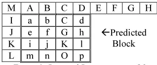
There are nine different Intra 4x4 Prediction modes namely, Vertical, Horizontal, DC, Diagonal-Down-Left, Diagonal-Down-Right, Vertical-Right, Horizontal-Down, Vertical-Left and Horizontal-Up, possible for a given 4x4 sMB in Intra 4x4 Prediction. The best mode is decided based on the Rate-Distortion Cost (RD-Cost) calculated for each mode Predictions.

In the process of RD-Cost calculation, each 4x4 sMB is subjected to all nine prediction modes. The 4x4 sMB is predicted by all nine different prediction techniques. The residue 4x4 sMB is found out by subtracting the predicted 4x4 sMB from original 4x4 sMB. There are nine sets of residue 4x4 sMBs, which are core forward transformed and quantized. The rate is calculated for each prediction mode by subjecting the quantized coefficients to variable length coding. The quantized coefficients are dequantized and core inverse transformed to get reconstructed residue 4x4 sMBs. These reconstructed residue 4x4 sMBs are added with already predicted 4x4 sMBs to get reconstructed 4x4 sMBs. The distortions are calculated between original 4x4 sMB and reconstructed 4x4 sMBs, by means of Sum of Absolute Error (SAE) or Sum of Squares of Error (SSE). For all 9 different modes, the RD-Cost are calculated by the following equation.

_ λ. (1)

The minimum RD-Cost will decide the mode for the given 4x4 sMB. The same process is continued for other fifteen 4x4 sMBs in a MB. This way of finalizing Intra 4x4 Prediction modes are followed by Joint Model (JM) Group [12] and x264 [13].

M A B C D E F G H

I a b C d

Predicted

Block

J e f G h

K i j K l

L m n O p

Figure 1: Pictorial Representation Of Neighbourhood In Intra Prediction

2.1 Vertical (VER) Mode

Vertical (VER) mode copies down the top four pixels (A, B, C and D) as predicted block shown below. As there are only copying operations, the computational complexity of Vertical Prediction is zero.

_

2.2 Horizontal (HOR) Mode

Horizontal (HOR) mode copies right the left four pixels (I, J, K and L) as predicted block shown below. As there are only copying operations, the computational complexity of Horizontal Prediction is zero.

_

2.3 DC Prediction (DC) Mode

DC Prediction (DC) mode finds the average of top four pixels (A, B, C and D) and left four pixels (I, J, K, and L), and copies the average in the entire predicted block.

4 ≫ 3

If the any of top or left four pixels are not

available, the is calculated by averaging the

available four pixels.

ܣݒ ൜ሺ_ሺ 2 _2ሻሻ_{≫ 2, ! "#$ %%&'%(')}≫ 2, ! "#$ %%&'%(')

If the current block is first in the frame, then is the predicted as half of Pixel bitwidth. The Pixel domain DC Predicted values are,

_

Considering the best case, the computational complexity is 8 additions and 1 shift operations.

2.4 Diagonal-Down-Left (DDL) Mode

In DDL mode Prediction, the pixel domain

values _ are calculated as follows.

_

1,1 1,2

1,2 1,3 1,3 1,41,4 2,4 1,3 1,4

1,4 2,4 2,4 3,43,4 4,4

There are only 7 unique pixel values which are calculated from neighbourhood pixels. The other 9 pixels are copied from the seven unique pixel values. The 7 unique pixels are calculated as follows.

1,1 ≪ 1 2 ≫ 2 1,2 ≪ 1 2 ≫ 2 1,3 ≪ 1 2 ≫ 2 1,4 ≪ 1 2 ≫ 2 2,4 ≪ 1 , 2 ≫ 2 3,4 , ≪ 1 2 ≫ 2 4,4 , ≪ 1 2 ≫ 2

The computational complexity of DDL

Prediction is 21 additions and 14 shifts.

2.5 Diagonal-Down-Right (DDR) Mode

In DDR mode Prediction, the pixel domain

values _ are calculated as below.

_

1,1 1,2

2,1 1,1 1,3 1,41,2 1,3 3,1 2,1

4,1 3,1 1,1 1,22,1 1,1

There are 7 pixel values which are calculated from neighbourhood pixels. Out of 7 pixel values, five are unique and two can be derived from DDL Prediction.

1,1 - ≪ 1 2 ≫ 2 1,2 - ≪ 1 2 ≫ 2

1,3 ≪ 1 2 ≫ 2 1,1 1,4 ≪ 1 2 ≫ 2 1,2 2,1 - ≪ 1 2 ≫ 2

3,1 ≪ 1 2 ≫ 2 4,1 ≪ 1 2 ≫ 2

The computational complexity of DDR

Prediction is 21 additions and 14 shifts.

2.6 Vertical-Right (VR) Mode

The pixel domain Vertical-Right (VR) mode Prediction values are given as follows.

_

1,1 1,2

2,1 2,2 1,3 1,42,3 2,4 3,1 1,1

VR mode has 10 distinct pixel values. Among that, only four are unique pixel values and the other six values can be derived from DDL and DDR Predictions.

1,1 - 1 ≫ 1 1,2 1 ≫ 1 1,3 1 ≫ 1 1,4 1 ≫ 1

2,1 - ≪ 1 2 ≫ 2 1,1 2,2 - ≪ 1 2 ≫ 2 1,2 2,3 ≪ 1 2 ≫ 2 1,1 2,4 ≪ 1 2 ≫ 2 1,2 3,1 - ≪ 1 2 ≫ 2 2,1 4,1 ≪ 1 2 ≫ 2 3,1

The computational complexity of VR Prediction is 26 additions and 16 shifts.

2.7 Horizontal-Down (HD) Mode

The pixel domain Horizontal-Down (HD) mode Prediction values are given below.

_

1,1 1,2

2,1 2,2 1,3 1,41,1 1,2 3,1 3,2

4,1 4,2 2,1 2,23,1 3,2

HD mode has 10 distinct pixel values given below. Out of those, 6 values can be derived from DDL and DDR Predictions.

1,1 - 1 ≫ 1

1,2 - ≪ 1 2 ≫ 2 1,1 1,3 - ≪ 1 2 ≫ 2 1,2 1,4 ≪ 1 2 ≫ 2 1,1 2,1 1 ≫ 1

2,2 - ≪ 1 2 ≫ 2 2,1 3,1 1 ≫ 1

3,2 ≪ 1 2 ≫ 2 3,1 4,1 1 ≫ 1

4,2 ≪ 1 2 ≫ 2 4,1

The computational complexity of HD Prediction is 26 additions and 16 shifts.

2.8 Vertical-Left (VL) Mode

The pixel domain Vertical-Left (VL) mode Prediction values are shown below.

_

1,1 1,2

2,1 2,2 1,3 1,42,3 2,4 1,2 1,3

2,2 2,3 1,4 3,42,4 4,4

VL mode has 10 distinct pixel values. Among that, only two are unique pixel values and the other

eight values can be derived from DDL and VR Predictions.

1,1 1 ≫ 1 1,2 1,2 1 ≫ 1 1,3 1,3 1 ≫ 1 1,4 1,4 1 ≫ 1

2,1 ≪ 1 2 ≫ 2 1,1 2,2 ≪ 1 2 ≫ 2 1,2 2,3 ≪ 1 2 ≫ 2 1,3 2,4 ≪ 1 2 ≫ 2 1,4 3,4 1 ≫ 1

4,4 ≪ 1 , 2 ≫ 2 2,4

The computational complexity of VL Prediction is 25 additions and 15 shifts.

2.9 Horizontal-Up (HU) Mode

The pixel domain Horizontal-Up (HU) mode Prediction values are shown below.

._

.1,1 .1,2

.1,3 .1,4 .1,3 .1,4.2,3 .2,4 .2,3 .2,4

HU mode has 7 distinct pixel values. Out of those, 5 pixel values can be derived from DDR and HD Predictions and one pixel value is L itself.

.1,1 1 ≫ 1 2,1

.1,2 ≪ 1 2 ≫ 2 3,1 .1,3 1 ≫ 1 3,1

.1,4 ≪ 1 2 ≫ 2 4,1 .2,3 1 ≫ 1 4,1 .2,4 ≪ 1 2 ≫ 2

The computational complexity of HU Prediction is 15 additions and 9 shifts.

For a 4x4 sMB, all possible predictions are done for all the nine modes. The computational Complexity of Intra 4x4 Prediction is 142 additions and 85 shifts in [12] and [13] (Table 2 and Table 3).

3. COMPLEXITY OF FINDING RESIDUE AND FORWARD TRANSFORM

Each predicted 4x4 sMB is subtracted from the original 4x4 sMB to get residue 4x4 sMBs. The computational complexity for one 4x4 sMB is 16 subtractions and zero shift. The computational complexity of finding residue for all nine prediction modes is 9x16 subtractions, i.e., 144 addition and zero shift operations in [12] and [13] (Table 3).

The residue sMB is core forward transformed using the following equation.

45)0) 2 1 61

2 61 61 6161 62 1 61

1 62 61 6162 61

%"7 2$ $0%"18#1)2

This core forward transform (It is a matrix multiplication) is simplified with additions and shifts only as follows.

for row = 1 to 4

f(row,1) = res(row,1) + res(row,4) f(row,2) = res(row,2) + res(row,3) f(row,3) = res(row,2) - res(row,3) f(row,4) = res(row,1) - res(row,4) end

for row = 1 to 4

g(row,1) = f(row,1) + f(row,2) g(row,2) = f(row,3) + f(row,4) << 1 g(row,3) = f(row,1) - f(row,2) g(row,4) = f(row,4) - f(row,3) << 1 end

for col = 1 to 4

h(1,col) = g(1,col) + g(4,col) h(2,col) = g(2,col) + g(3,col) h(3,col) = g(2,col) - g(3,col) h(4,col) = g(1,col) - g(4,col) end

for col = 1 to 4

RES(1,col) = h(1,col) + h(2,col) RES(2,col) = h(3,col) + h(4,col) << 1 RES(3,col) = h(1,col) - h(2,col) RES(4,col) = h(4,col) - h(3,col) << 1 end

Algorithm to perform core forward transform in [12] and [13]

The computational complexity of core forward transform of one residue 4x4 sMB is 64 additions and 16 shifts. For all nine modes, the computational complexity is 9x64 additions and 9x16 shifts, i.e., 576 addition and 144 shift operations in [12] and [13] (Table 3).

4. PROPOSED METHOD WITH COMPUTATIONAL COMPLEXITY

It is clearly found that there are 24 unique pixel values for all nine intra 4x4 modes. The number of unique pixel values corresponding to each mode is listed in the Table 1.

1,1 , 4 ≫ 3 1,1 ≪ 1 2 ≫ 2

1,2 ≪ 1 2 ≫ 2 1,3 ≪ 1 2 ≫ 2 1,4 ≪ 1 2 ≫ 2 2,4 ≪ 1 , 2 ≫ 2 3,4 , ≪ 1 2 ≫ 2 4,4 , ≪ 1 2 ≫ 2 1,1 - ≪ 1 2 ≫ 2 1,2 - ≪ 1 2 ≫ 2 2,1 - ≪ 1 2 ≫ 2

3,1 ≪ 1 2 ≫ 2 4,1 ≪ 1 2 ≫ 2 .2,4 ≪ 1 2 ≫ 2 1,1 - 1 ≫ 1 1,2 1 ≫ 1 1,3 1 ≫ 1 1,4 1 ≫ 1 1,4 1 ≫ 1 3,4 1 ≫ 1 1,1 - 1 ≫ 1 2,1 1 ≫ 1 3,1 1 ≫ 1 4,1 1 ≫ 1

Mode Number of unique pixel values

DC Prediction 1

Diagonal-Down-Left Prediction 7 Diagonal-Down-Right Prediction 5 Vertical-Right Prediction 4 Horizontal-Down Prediction 4 Vertical-Left Prediction 2 Horizontal-Up Prediction 1

Total 24

Table 1 Number of unique pixel values for each mode

The other pixel values are copied from the already calculated pixel values by the above-said 24

equations. Thus reduces the computational

complexity to 67 addition and 37 shift operations. But those 24 equations are split intelligently and modified as follows.

1 1 1 1 1 , , 1 , , 1 - - 1 - - 1 1 1 1

1,2 ≫ 1 1,3 ≫ 1 1,4 ≫ 1 1,1 - ≫ 1 1,4 ≫ 1 3,4 ≫ 1 1,1 - ≫ 1 2,1 ≫ 1 3,1 ≫ 1 4,1 ≫ 1

1,1 , ≫ 3 1,1 ≫ 2

1,4 ≫ 2 2,4 , ≫ 2 3,4 , , ≫ 2 4,4 , ≪ 1 1 ≫ 2 1,1 - - ≫ 2 1,2 - ≫ 2 2,1 - ≫ 2 3,1 ≫ 2 4,1 ≫ 2 .2,4 ≪ 1 1 ≫ 2

Now, computational complexity of finding pixel domain predictions for all nine modes is 42 addition and 26 shift operations (Table 4).

The facts of transform domain predicted coefficients are given below.

1) The pixel domain predicted 4x4 sMB of

each mode has spatial redundancy. When predicted sMB is subtracted from original sMB to form residue sMB, this spatial redundancy is not utilized/exploited. So, the pixel domain predicted values are core forward transformed to exploit the spatial redundancy.

2) The additive property of Core Forward

Transform is shown below.

! – ! 6 !

3) Using the above-said equation and the

spatial redundancy of pixel domain predicted sMB, certain selected transform domain predicted sMB coefficients are directly calculated.

The novel approach of finding transform domain residue is calculated by subtracting the

transform domain predicted values from

transform domain original values, that is,

–

.

Finding ORG and PRED & RES are explained here-after.

4.1 Transform Of Original

The original 4x4 sMB is core-forward transformed and its computational complexity is 64 additions and 16 shifts.

, 2 3 #0: 3 2$

45)0) , &1 ;#0) 2#04%07 $0%"12#0<)7 #0&:&"%'

4.2 Vertical Mode Residue

The transform domain Vertical predicted values are calculated as below.

_! 2 3 _ 3 2$ 11 12

0 0 13 140 0 0 0

0 0 0 00 0

The four transform coefficients are calculated as follows.

11 ≪ 2 12 1 ≪ 1 1 ≪ 2 13 6 ≪ 2 14 1 6 1 ≪ 1 ≪ 2

where,

1 6 1 6

The computational complexity to find transform domain Vertical Prediction mode coefficients is 8 additions and 6 shifts. The transform domain residue for Vertical Prediction Mode is calculated by subtracting these four transform coefficients from original transform coefficients.

_/

>,&, ? 6 _!&, ?, & 1, ? 1 $# 4 _{,&, ?, & 2 $# 4, ? 1 $# 4}

The computational complexity to find transform domain residue coefficients of Vertical Prediction mode is 4 additions and zero shifts.

4.3 Horizontal Mode Residue

The transform domain Horizontal predicted values are calculated as below.

_! 2 3 _ 3 2$ 11 0 21 0 0 00 0 31 0 41 0 0 00 0

The four transform coefficients are calculated as follows.

11 ≪ 2 21 1 ≪ 1 1 ≪ 2 31 6 ≪ 2 41 1 6 1 ≪ 1 ≪ 2

where,

The computational complexity to find transform domain Horizontal Prediction mode coefficients is 8 additions and 6 shifts. The transform domain residue for Horizontal Prediction Mode is calculated by subtracting these four transform coefficients from original transform coefficients.

_/

>,&, ? 6 _!&, ?, & 1 $# 4, ? 1 _{,&, ?, & 1 $# 4, ? 2 $# 4}

The computational complexity to find transform

domain residue coefficients of Horizontal

Prediction mode is 4 additions and zero shifts.

4.4 DC Mode Residue

The unique and only one pixel domain predicted

value is , where 1,1 (Refer Page 4).

The transform domain coefficients are calculated as follows.

_! 2 3 _ 3 2$ 11 0

0 0 0 0 0 0 0 0

0 0 0 0 0 0

where, 11 1,1 ≪ 4

The computational complexity to find transform domain DC Prediction mode coefficients is zero additions and 1 shift. The transform domain residue for DC Prediction Mode is calculated by subtracting this one transform coefficient from original transform coefficient.

_/ >,&, ? 6 11, & 1, ? 1 _{,&, ?, & 1 $# 4, ? 1 $# 4}

The computational complexity to find transform domain residue coefficients of DC Prediction mode is 1 addition and zero shifts.

4.5 Diagonal-Down-Left Mode Residue

The transform domain DDL predicted values are

derived as follows: _! 2 3 _ 3 2$

_!

11 12

12 22 13 1423 24 13 23

14 24 33 3434 44

The ten unique transform coefficients are calculated as follows.

11 _11 _08 _10 12 _12 ≪ 1 _09 13 _00 6 _02 14 _12 6 _05

22 _00 _04 ≪ 2 6 _08 6 _07 23 _01 6 _13 ≪ 1 6 _05

24 _00 6 _04 ≪ 1 _02 6 _04 33 _11 6 _02 6 _10

34 _12 _13 6 _09 44 _00 _02 ≪ 3 6 _04

≪ 2 6 _07

where,

_00 1,1 4,4 _01 1,1 6 4,4 _02 1,3 2,4 _03 1,3 6 2,4 _04 1,2 3,4 _05 1,2 6 3,4 _06 1,4 ≪ 2

_07 1,4 ≪ 3 1,4 ≪ 1 _08 _02 ≪ 1 _02 _09 _05 ≪ 1 _05 _10 _04 ≪ 1

_11 _00 _06 _12 _01 _03 _13 _03 ≪ 1

The computational complexity to find transform domain coefficients of DDL Prediction mode is 31 additions and 13 shifts. The transform domain residue for DDL Prediction Mode is calculated by subtracting these transform coefficients from original transform coefficient.

_/ ,&, ? 6 _!&, ?, & 1 $# 4, ? 1 $# 4

The computational complexity to find transform domain residue coefficients of DDL Prediction mode is 16 additions and zero shifts.

4.6 Diagonal-Down-Right Mode Residue

The transform domain DDR predicted values are

derived as follows: _! 2 3 _ 3 2$

_!

611 612

612 622 661323 661424

613 623

614 624 663433 663444

The ten unique transform coefficients are calculated as follows.

_!1,1 _05 _11 _12 _!1,2 6 _03 6 _08 ≪ 1 _!1,3 _01 6 _04 _!1,4 _02 6 _08

_!2,2 _05 _10 6 _14 6 _13 ≪ 1

_!2,3 _07 6 _15 ≪ 1 6 _02 _!2,4 _00 6 _04 _11

6 _13

_!3,3 _12 6 _11 6 _04 _!3,4 _03 6 _06 6 _07

6 _15

_!4,4 _14 6 _01 6 _04 ≪ 3 _10

_00 1,1 3,1 _01 1,2 4,1 _02 1,1 6 3,1 _03 _02 ≪ 1 _02 _04 1,2 2,1 _05 _04 ≪ 1 _04 _06 1,2 6 2,1 _07 1,2 6 4,1 _08 _06 _07 _09 1,1 ≪ 2

_10 1,1 _09 ≪ 1 _11 _00 ≪ 1

_12 _01 _09 _13 _01 ≪ 1 _14 _11 ≪ 1 _15 _06 ≪ 1

The computational complexity to find transform domain coefficients of Diagonal-Down-Right Prediction mode is 32 additions and 12 shifts. The transform domain residue for Diagonal-Down-Right Prediction Mode is calculated by subtracting these transform coefficients from original transform coefficient.

_/ ,&, ? 6 _!&, ?, & 1 $# 4, ? 1 $# 4

The computational complexity to find transform domain residue coefficients of Diagonal-Down-Right Prediction mode is 16 additions and zero shifts.

4.7 Vertical-Right Mode Residue

The transform domain VR predicted values are

derived as follows: _! 2 3 _ 3 2$

All the transform coefficients _! calculated

as follows.

_!1,1 _02 _05 _08 _!1,2 _13 6 _10 ≪ 1 _!1,3 _02 6 _08 _!1,4 6_10 6 _12 _!2,1 _11 _16 _18 _!2,2 _20 6 _03 ≪ 1 _09 _!2,3 _11 _13 6 _18

_!2,4 _04 6 _03 _05 6 _09 ≪ 1 _!3,1 _00

_!3,2 _18 6 _14 ≪ 1 _16 _!3,3 _00 _06

_!3,4 _17 6 _14 6 _18 ≪ 2 _!4,1 _15 _17 _19

_!4,2 _06 6 _01 ≪ 1 6 _04 6 _07 _!4,3 _15 6 _12 6 _19

_!4,4 _08 6 _01 6 _20

where,

$8_00 1,4 3,1 $8_01 1,4 6 3,1 $8_02 2,1 1,2 $8_03 2,1 6 1,2 $8_04 1,1 1,1 $8_05 1,1 6 1,1 $8_06 1,3 6 1,1

$8_07 $8_04 ≪ 1 _00 $8_00 6 $8_02 _01 _00 6 $8_02 _02 $8_00 $8_02 _03 $8_00 _02 _04 1,3 1,1 _05 $8_07 _04 ≪ 1 _06 $8_07 6 _04 ≪ 1 _07 1,2 1,2 _08 _07 ≪ 1 _09 _08 _07 _10 $8_01 6 $8_03 _11 $8_01 _10 _12 $8_05 6 $8_06 _13 _12 ≪ 1 _12 _14 $8_01 $8_03 _15 _14 $8_03 _16 $8_05 $8_06 _17 _16 ≪ 1 _16 _18 1,2 6 1,2 _19 _18 ≪ 1 _18 _20 $8_04 $8_07

The computational complexity to find transform domain coefficients of Vertical-Right Prediction mode is 55 additions and 12 shifts. The transform domain residue for Vertical-Right Prediction Mode is calculated by subtracting these transform coefficients from original transform coefficient.

_/ ,&, ? 6 _!&, ?, & 1 $# 4, ? 1 $# 4

The computational complexity to find transform domain residue coefficients of Vertical-Right Prediction mode is 16 additions and zero shifts.

4.8 Horizontal-Down Mode Residue

The transform domain VR predicted values are

derived as follows: _! 2 3 _ 3 2$

All the transform coefficients _

calculated as follows.

_!1,1 _12 _23 _21 _!1,2 _25 6 _18 _!1,3 6_13

_!1,4 _19 _25 ≪ 1 _25 _!2,1 _16 ≪ 1 _27 _!2,2 _20 6 _15 ≪ 1 _22 _!2,3 _09 6 _17 ≪ 1 _25 _!2,4 _14 _24

≪ 1 6 _06 6 _08 _!3,1 _12 6 _21

_!3,2 _27 6 _18 6 _09 _!3,3 _24 6 _13

_!3,4 _19 6 _10 6 _09 ≪ 1 6 _09 _!4,1 _16 6 _10

_!4,2 _06 6 _15 6 _22 6 _23 ≪ 1

_!4,3 _26 6 _17 6 _09 _26 ≪ 1 _!4,4 _14 6 _20 _21

where,

_01 1,2 6 4,1 _02 1,1 4,1 _03 1,1 6 4,1 _04 1,1 3,1 _05 1,1 6 3,1 _06 1,1 3,1 _07 1,1 6 3,1 _08 2,1 2,1 _09 2,1 6 2,1 _10 _05 _07 _11 _05 6 _07 _12 _00 _02 _13 _00 6 _02 _14 _13 _00 _15 _12 _02 _16 _01 _03 _17 _01 6 _03 _18 _16 _03 _19 _17 _01 _20 _04 ≪ 1 _04 _21 _08 ≪ 1 _22 _21 _08 _23 _04 _06 ≪ 1 _24 _04 6 _06 ≪ 1 _25 _11 _09 _26 _11 6 _09 _27 _10 ≪ 1 _10

The computational complexity to find transform domain coefficients of Horizontal-Down Prediction mode is 56 additions and 12 shifts. The transform domain residue for Horizontal-Down Prediction Mode is calculated by subtracting these transform coefficients from original transform coefficient.

_/ ,&, ? 6 _!&, ?, & 1 $# 4, ? 1 $# 4

The computational complexity to find transform domain residue coefficients of Horizontal-Down Prediction mode is 16 additions and zero shifts.

4.9 Vertical-Left Mode Residue

The transform domain VL predicted values are

derived as follows: _! 2 3 _ 3 2$

All the transform coefficients !_

calculated as follows.

_!1,1 _10 _21 _22 _!1,2 _14 ≪ 1 6 _26 _!1,3 _10 6 _21 _!1,4 _14 _19 _!2,1 _07 _16 _18

_!2,2 _12 6 _06 ≪ 1 6 _06 6 _20 _!2,3 _16 6 _07 _26

_!2,4 _12 6 _04 _21 _21 6 _22 ≪ 1

_!3,1 _11

_!3,2 _15 6 _07 ≪ 1 6 _18 _!3,3 _11 6 _23

_!3,4 _07 ≪ 2 _15 6 _25 _!4,1 _24 _17 _25

_!4,2 _04 _06 _13 _23 ≪ 1 _!4,3 _17 6 _24 6 _19

_!4,4 _13 _20 6 _21

where

_00 1,2 2,4 _01 1,2 6 2,4 _02 1,1 3,4 _03 1,1 6 3,4 _04 1,3 1,4 _05 1,3 6 1,4 _06 1,4 1,3 _07 1,4 6 1,3 _08 1,4 1,2 _09 1,4 6 1,2 _10 _00 _02 _11 _00 6 _02 _12 _10 _00 _13 _11 6 _02 _14 _01 _03 _15 _01 6 _03 _16 _01 _14 _17 _15 6 _03 _18 _09 _05 _19 _09 6 _05 _20 _08 ≪ 1 _08 _21 _06 ≪ 1

_22 _04 _08 ≪ 1 _23 _04 6 _08 ≪ 1 _24 _07 ≪ 1 _07 _25 _18 ≪ 1 _18 _26 _19 ≪ 1 _19

The computational complexity to find transform domain coefficients of Vertical-Left Prediction mode is 56 additions and 14 shifts. The transform domain residue for Vertical-Left Prediction Mode is calculated by subtracting these transform coefficients from original transform coefficient.

_/ ,&, ? 6 _!&, ?, & 1 $# 4, ? 1 $# 4

The computational complexity to find transform domain residue coefficients of Vertical-Left Prediction mode is 16 additions and zero shifts.

4.10 Horizontal-Up Mode Residue

The transform domain HU predicted values are

derived as follows: ._! 2 3 ._ 3 2$

All the transform coefficients "_

calculated as follows.

._!1,1 ._00 ._02 ._04 ._09 ≪ 1

._!1,2 ._06 ._03 ._11 ._!1,3 ._01

._!1,4 ._14 ._10

._!2,1 ._00 ._02 6 ≪ 1 ._02 6 ≪ 3

._!3,4 ._07 ._02 6 ._10 ._!4,1 ._00 6 ._02

._!4,2 ._06 6 ._15 ≪ 2 6 ._15 ._12 ._!4,3 ._01 6 ._03 6 ._05

≪ 2 ._03

._!4,4 ._07 ._08 ._13 ≪ 1 ._13

where,

._00 2,1 3,1 ._01 2,1 6 3,1 ._02 3,1 4,1 ._03 3,1 6 4,1 ._04 4,1 .2,4 ._05 4,1 6 .2,4 ._06 2,1 ._00 ._07 ._01 6 3,1 ._08 ._04 6 ._09 ≪ 1

._10 ._05 ≪ 1 ._05 ._11 ._05 6 ._09 ._12 4,1 ._08 ._13 4,1 6 ._08

._14 ._07 ._03 ≪ 1 ._03 ._15 ._02 6 ._08

The computational complexity to find transform domain coefficients of Horizontal-Up Prediction mode is 51 additions and 16 shifts. The transform domain residue for Horizontal-Up Prediction Mode is calculated by subtracting these transform coefficients from original transform coefficient.

._/ ,&, ? 6 ._!&, ?, & 1 $# 4, ? 1 $# 4

The computational complexity to find transform domain residue coefficients of Horizontal-Up Prediction mode is 16 additions and zero shifts.

5. COMPARISON AND INFERENCES OF THE PROPOSED METHOD

The computational complexity of reference software and the proposed method are compared here. The computational complexity of Pixel domain Intra 4x4 Prediction for all the nine prediction modes in the reference software [12] and [13] are tabulated in the table 2.

The reference software does the pixel domain prediction first, and then finds the residue and last it does the forward transform for all nine modes. In that order, the computational complexity of the existing reference software is listed in the table 3.

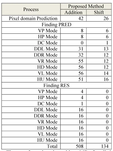
The proposed method calculates the selective pixel domain values, the selective transform domain coefficients and finds the transform domain residue coefficients. The computational complexity of the proposed method is listed in table 4.

Table 2 Complexity of Pixel domain Intra 4x4 prediction in reference software

Prediction Type Reference Software Addition Shifts

Vertical 0 0

Horizontal 0 0

DC 8 1

Diagonal-Down-Left 21 14 Diagonal-Down-Right 21 14 Vertical-Right 26 16 Horizontal-Down 26 16 Vertical-Left 25 15 Horizontal-Up 15 9 Total 142 85

Table 3 Complexity of Reference software during Intra 4x4 prediction

Process Reference Software Addition Shift Pixel domain Prediction 142 85

Finding Residue 144 0 Forward Transform 576 144 Total 862 229

Table 4 Complexity of Proposed method during Intra 4x4 prediction

Process Proposed Method Addition Shift Pixel domain Prediction 42 26

Finding PRED

VP Mode 8 6

HP Mode 8 6

DC Mode 0 1

DDL Mode 31 13 DDR Mode 32 12 VR Mode 55 12 HD Mode 56 12 VL Mode 56 14 HU Mode 51 16

Finding RES

VP Mode 4 0

HP Mode 4 0

DC Mode 1 0

DDL Mode 16 0

DDR Mode 16 0

VR Mode 16 0 HD Mode 16 0 VL Mode 16 0 HU Mode 16 0 Total 508 134

just by copying from available 24 unique pixel values.

6. CONCLUSION

In H.264 Encoder, the computational

complexity of Intra4x4 mode decision by RD-Cost method is higher than any other methods. But RD-Cost method gives best results. Especially, the process of predicting the intra 4x4 prediction for all the nine modes, finding the residue and forward transforming will take more complexity in terms of addition and shifts. Every MB in the frame of the sequence is subjected to do this process repeatedly for all its sixteen sMBs. This paper proposed a method to find transform domain residue values directly with reduced computational complexity. The proposed method used (i) the unique equations for prediction, (ii) the additive property of core forward transform and (iii) the spatial redundancy of pixel domain predicted values. Thus the proposed method reduced the computational complexity into 59% addition and 59% shift

operations, thus saved 41% computational

complexity. But the proposed method did not compromise the accuracy of the results, thus maintaining the same quality and bitrate. The same method can be extended to Intra 16x16 Prediction, Intra 8x8 Prediction and Intra Chroma Predictions also in H.264 Encoder.

ACKNOWLEDGMENT

The author thanks RiverSilica Technologies Private Limited, INDIA for their encouragement and support.

REFRENCES:

[1] T. Wiegand, G. J. Sullivan, G. Bjontegaard, and A. Luthra, “Overview of the H.264/AVC video

coding standard,” IEEE Transactions on

Circuits and Systems for Video Technology., Vol. 13, No. 7, pp. 560–576, July 2003. [2] A. Joch, F. Kossentini, H. Schwarz, T.

Wiegand, and G. J. Sullivan, “Performance

comparison of video standards using

Lagrangian control,” in Proc. IEEE Int. Conf.

Image Process., pp. 501–504, 2002.

[3] W. Zouch, A. Samet, M. A. Ben Ayed, F

Kossentini, N. Masmoudi, “Complexity

Analysis of Intra Prediction in H.264/AVC”,

16th International Conference on Micro Electronics Proceedings, on December 6-8, 2004.

[4] Mustafa Parlak, Yusuf Adibelli, and Ilker

Hamzaoglu, “A Novel Computational

Complexity and Power Reduction Technique

for H.264 Intra Prediction”, IEEE Transactions

on Consumer Electronics, pp. 2006 – 2014, Vol. 54, No. 4, November 2008.

[5] Y. Adibelli, M. Parlak, and I. Hamzaoglu, “A Computation and Power Reduction Technique

for H.264 Intra Prediction”, 13th Euromicro

Conference on Digital System Design: Architecture, Methods and Tools, pp. 753 – 760, 2010.

[6] E. Sahin, I. Hamzaoglu, “An Efficient Hardware Architecture for H.264 Intra Prediction

Algorithm”, Design, Automation & Test in

Europe Conference & Exhibition, 16-20 April 2007.

[7] Y. Lai, T. Liu, Y. Li, C. Lee, “Design of An Intra Predictor with Data Reuse for

High-Profile H.264 Applications”, IEEE ISCAS, pp.

3018 – 3021, May 2009.

[8] F. Pan, X. Lin, S. Rahardja, K. Lim, Z. Li, S. Dajun Wu, “Fast Mode Decision Algorithm for Intra Prediction in H.264/AVC Video Coding”,

IEEE Transactions on CAS for Video Technology, Vol. 15, No. 7., pp 813 – 822, July 2005.

[9] I. Choi, J. Lee, B. Jeon, “Fast Coding Mode Selection With Rate-Distortion Optimization

for MPEG-4 Part 10 AVC/H.264”, IEEE

Transactions on CAS for Video Technology,

Vol. 16, No. 12, pp 1557 – 1561, December 2006.

[10] A. Elyousfi, A. A. Tamtaoui, and E. Bouyakhf, “A New Fast Intra Prediction Mode Decision

Algorithm for H.264/AVC Encoders”, World

Academy of Science, Engineering and Technology, 2007.

[11] Iain E. Richardson, “The H.264 – Advanced Video Compression Standard” – Second Edition – A John Wiley and Sons, Ltd., Publication, 2010.

[12] Joint Video Team, JM Reference Software V17.1 - iphome.hhi.de/suehring/tml/.

[13] x264 Encoder Open Source –