APPLYING HYBRID GENETIC ALGORITHMS TO RECOVER
FOCAL LENGTH, CAMERA MOTION AND 3D MODELS
FROM SILHOUETTES
1AMINE MOUAfi, 1RACHID BENSLIMANE AND 2AZIZA EL OUAAZIZI
1
Laboratoire de Transmission et Traitement d’Information, École Supérieure de Technologie, Université Sidi Mohamed Ben Abdellah, Route d’Imouzzer B.P. 2427, Fez, Morocco.
2LIMAO, Faculté Poly-disciplinaire de Taza, Université Sidi Mohamed Ben Abdellah, Route d’Oujda,
B.P. 1223, Taza, Morocco.
E-mail: [email protected], [email protected], [email protected]
ABSTRACT
In this paper, a hybrid method is applied to recover parameters and motion of camera from a set of silhouettes of an object taken under circular motion. Camera parameters can be obtained by maximizing the total coherence between all silhouettes. Two optimization methods, the Powell optimizer (PO) and the Genetic algorithms (GA), are applied to maximize the silhouette coherence and their performances are compared for several experiments. To take advantage of the strengths of the two methods, we developed a hybrid method that combines the genetic algorithm and the Powell optimizer to improve the performances in term of convergence speed and accuracy. The recovered parameters are used for 3D image-based modeling to obtain high fidelity 3D reconstruction.
Keywords: Hybrid Genetic Algorithms, Powell Optimizer, Silhouette Coherence, Parameters Estimation,
Circular Motion
1. INTRODUCTION
Acquiring 3D information from images has always been a hot research topic in 3D computer vision and recently, it has attracted more and more interest because of its potential applications such as computer games, augmented reality and cultural heritage preservation. In 3D computer vision, it is necessary to know the relationship between the 3D object coordinates and the image coordinates. This transformation is determined in the camera calibration step by recovering the camera intrinsic parameters and the relative pose of the camera.
Recovering camera parameters and motion from image sequences without using any calibration patterns can be classified into two approaches: the feature-based and silhouette-based approaches. In the feature-based approach, structure from motion algorithm [1] determines the camera parameters and the 3D structure of the object simultaneously from the feature correspondences [2], [3]. These methods would therefore be not applicable to smoothed objects with low texture. In addition to feature correspondences, silhouettes also offer important clues for determining both motion and shape. It is especially the case when the object being viewed is composed of non textured smooth surfaces like
pottery and sculptures. For this kind of object, silhouettes are the most predominant and stable image feature.
Silhouette-based approaches generally exploit epipolar tangents [4], [5], to locate the images of the frontier points for deriving point correspondences between images. Hernandez et al. [6] considered the problem of recovering both the focal length and the camera motion under circular motion from silhouettes. They extended the idea of exploiting the epipolar tangents [5] to the concept of silhouette coherence, which measures how well a set of silhouettes corresponds to the projections of the visual hull. The author performed camera calibration by maximizing the silhouette coherence in optimization procedure.
The Powell optimizer [7] was able to quickly reach the optimal solution for silhouette coherence maximization. However, we encountered difficulties in robustness when the initial guess for parameters are far away from the optimal solution, and when the desired global maximum was hidden by many local maxima.
Darwinian ‘’Natural selection’’ theory, according to which individuals that are better fit to a given environment are more likely to survive. GA are problem-independent and can process information generated at previous stages of a search process. They comprise concepts such as natural selection, quick exploration, and information collection in a design space. In contrast to most of classical optimization methods, GA require no initial guess for parameters and can avoid being trapped in local optimal solutions as shown in our previous work [10]. These characteristics make the GA powerful tools for solving optimization problems.
In this paper, two optimization methods, the Powell optimizer (PO) and a Genetic algorithm (GA), are applied to maximize the silhouette coherence and their performances are compared for several experiments. To take advantage of the strengths of the two methods, we developed a hybrid method that combines the genetic algorithms (GA) and Powell optimizer (PO) to improve the performance of the optimization procedure.
The remainder of this paper is organized as following: in Section 2 we present the circular motion parameterization. In section 3 we present the silhouette coherence measure and its practical implementation. In section 4 and 5, three optimization methods including a Powell optimizer, Genetic Algorithms, and our hybrid GA-PO, are described, applied and compared for several tests in term of convergence and accuracy. In section 6 we build 3D models with the recovered parameters.
2. CIRCULAR MOTION
PARAMETERIZATION
2.1 Camera Model
We consider a pinhole camera model. The geometry of a pinhole camera model is illustrated in Fig. 1. Let M = (x, y, z) be a 3D point in an object frame and m = (u, v) the corresponding image point in the image frame. The central projection of a 3D scene point M onto its 2D image point m can be written with the following linear equation using homogeneous coordinates:
[ ]
R
T
M
K
PM
m
≈
≈
(1)
Where
=
1
0
0
0
0
0 0
v
fy
u
fx
K
(2)
The projection matrix P is a 3×4 matrix defined up to a scalar factor that captures both the extrinsic and intrinsic camera parameters. R and T representing the rotation and translation between the world coordinate system and the camera coordinate system respectively. K is the camera calibration matrix. The parameters fy and fx represent the focal lengths measured in pixel units, with the aspect ratio defined as r = fy/fx, (u0,v0 )
represents the coordinates of the principal point.
In this paper, the aspect ratio is assumed to be one (r=1), the principal point (u0,v0) is considered to
be the center of the image. The only intrinsic parameter that we consider is the focal length f.
Figure 1: The geometry of a pinhole camera model
2.2 Circular Motion Parameterization
Circular motion is a practical setup for image-based modeling. A circular motion image sequence can be obtained equivalently in two ways. The most common, and the one used in our real image experiments, is the case of a static camera viewing an object rotating on a turntable. A second method is that of a camera rotating around a fixed axis and pointing at a static object. Figure 2 shows the 3D geometry of circular motion. The camera matrix P1
of the first view can be written as:
] t R [ K =
P1 1 1 (2)
where K is the camera calibration matrix, R1 and t1
Figure 2: Circular Motion Parameterization
After rotating by ω about the axis
a
(θa, φa), thecamera matrix Pω of the second view can be
achieved by post-multiplying [R1|t1] with Ra(ω):
)
(
R
]
t
R
[
K
=
P
ω 1 1 aω
(3)Suppose that the circular motion image sequence consists of n views and the camera matrices for each view is denoted by Pi i=1,…,n,
from (2) and (3) we have
) ( R P =
Pi 1 a
ω
i (4)where ωi denotes the rotation angle between the ith
and the first view, the rotation matrix Ra(ωi) is
written as a function of ωi and the axis a(θa, φa) as
follow: − − − + − = i i x i y i x i i z i y i z i z z y z x z y y y x z x y x x i i a a a a a a a a a a a a a a a a a a a a a R ω ω ω ω ω ω ω ω ω ω ω cos sin sin sin cos sin sin sin cos ) cos 1 ( ) ( 2 2 2 (5)
the rotation axis
a
is written in function ofspherical coordinates (θa, φa):
(
a a a a a)
a= sinθ cosφ ,sinθ sinφ ,cosθ
the translation is written in function of an angle
α
t (the angle formed between the camera viewing direction and the z-axis see Fig. 2) as follow:(
t a)
t
1=
sin
α
,
0
,
cos
α
For n views, we parameterize the circular motion with n+3 parameters: the focal length f, the translation direction angle αt, the rotation axis
coordinates (θa, φa), the n-1 camera angle steps ωi.
In this paper, our goal is to recover the projection matrices Pi of a set of silhouettes Si of an object
taken under circular motion as the set of n+3 parameters: 1 , , 1 ), , , , , ( = −
= f i n
v
θ
aϕ
aα
tω
i K3. SILHOUETTE COHERENCE
Given a set of silhouettes Si, i = 1,…,n of a
same 3D object taken from different points of view, and the corresponding set of camera projection matrices Pi. Let Vh denote the reconstructed visual
hull1 using the set of silhouettes Si, and Svi denote
the reconstructed visual hull silhouettes. We would like to evaluate the coherence between the silhouette Si and all the other silhouettes Sj≠i that
contributed to the reconstructed visual hull Vh.
Figure 3: Visual Hull Reconstruction From A Set Of Silhouettes. Left: Silhouettes Obtained By Projecting The
Original Object Back Into Cameras. Right: The Reconstructed Visual Hull Using These Silhouettes.
We assume that the silhouettes segmentation and the projection matrices are exact. We say that the silhouette Si is coherent with all the other
silhouettes Sj≠i if the reconstructed visual hull
silhouettes Svi and the original silhouette Si are
exactly the same (Si = Svi). Two examples of
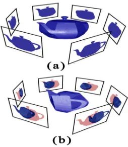
coherent and non-coherent silhouettes are shown in Fig.4 and Fig. 5.
Figure 4: Two Examples Of Different Silhouette Coherence. (A) Perfect Coherent Silhouette. (B) Low
Silhouette Coherence.
1 visual hull is an outer approximation of the observed solid,
[image:3.612.353.480.491.637.2]Figure 5: The Original Silhouettes Si Superposed With
The Visual Hull SilhouettesSv
i. The Red Region Indicates
Non Coherent Silhouette Pixels.
3.1 Measure Of Silhouette Coherence
To evaluate the coherence between silhouettes, some kind of similarity measurement between the original silhouette Si and the reconstructed visual
hull silhouettes Svi is needed. Hernandez [6] defines
this measure of coherence as the ratio of the silhouette contour lengths:
(
)
] 1 , 0 [ )
,
( ∈
∂ ∂ ∩ ∂ =
∫
∫
i i i
i i S S C
ν ν
(6)
where ∂i denote the contour of the original
silhouette Si and ∂vi the contour of the
reconstructed visual hull silhouette Svi.
To compute the total coherence between all the silhouettes, we compute the mean coherence of each silhouette with the (n-1) other silhouette [6].
∑
=
=
ni
i i j
i
SC
C
S
S
n
S
S
C
1
)
,
(
1
)
,...,
(
ν (7)If the silhouettes segmentation and the projection matrices are exact then:
1
)
,...,
(
i j=
SC
S
S
C
(8)
3.2 Silhouette coherence implementation
The simplest implementation of silhouette coherence, would be the following: i) compute the reconstructed visual hull defined by the silhouettes, ii) project the reconstructed visual hull back into the cameras, iii) compare the reconstructed visual hull silhouettes to the original ones. The major drawback of this approach is the computation time. Since the reconstruction of the visual hall will take several minutes, and if we want accurate projected silhouettes, we need a high resolution 3D model of the visual hull, which is computationally very expensive and not appropriate for an iterative optimization process. In addition, we are not interested in 3D model in itself but in the comparison between its silhouettes with the original silhouettes. Therefore, it is a waste of time to build the visual hull completely when only some views of
it are required. The imaged-based visual hull (IBVH) technique [11] does not compute a 3D representation of the reconstructed visual hull but only 2D views of it. To take advantage of epipolar geometry, 3D ray intersections required to construct the VH are reduced to 2D line intersections, which simplify the computation.
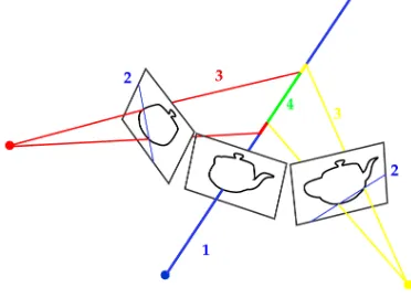
The implementation of silhouette coherence will be as following: for each 2D point in contour, compute the intersection between its corresponding optic ray and the visual hull by a ray-casting approach, this is equivalent to (see Figure 6):
1. project the optic ray into each silhouette 2. compute the 2D intersection intervals
between the projected ray and each silhouette
3. back project all the 2D intervals onto the original 3D optic ray,
4. Compute the intersection on the 3D optic ray of all the intervals of all the silhouettes
For any optic ray, we have a set of remaining depth intervals, possibly empty, which represent the intersection between the optic rays and the implicit visual hull.
Figure 6: 2D Computation Steps, (1) Project The 3D Optic Ray, (2) Compute The 2D Intersection Intervals Between The 3D Optic Ray And Each Silhouette, (3) Back Project All 2D Intervals Onto The 3D Optic Ray,
(4) The Intersection On The 3D Optic Ray (Green Segment).
4 OPTIMIZATION ROUTINES
In order to exploit silhouette coherence for recovering camera parameters and motion under circular motion, the idea is to use the silhouette coherence measure CSC as the cost in an
optimization procedure. In this section, three optimization methods, including a Powell optimizer, Genetic Algorithms, and a hybrid GA-PO, are applied to maximize CSC (Eq. 7) and
[image:4.612.323.509.390.525.2]4.1 Powell Optimizer (PO)
The first optimization method used here is the Powell direction set method. The Powell optimizer applied in this paper is the version described in [12, 13] in which starting points and a set of independent search directions are provided to the program. In each iteration the method serially performs a sequence of line minimizations along the various directions in the space of parameters. At the end of each iteration the method replaces one of the original directions with the line joining the starting and ending points. A special care is taken to ensure that the directions remain linearly independent. This version of the Powell optimizer is applied to the Silhouette coherence maximization problem. Although there are many other implementations of the PO such as described in [14, 15], the current work does not intend to include a comparative study of the merits of each of these implementations.
4.2 Genetic Algorithms (GA)
When solving an optimization problem using GA, each solution is usually coded as an alphabet string of finite length called chromosome. Each string or chromosome is considered as an individual. A collection of N individuals is called population. GA start with a randomly generated population of size N, in each iteration of the algorithm, a new population of the same size is generated from the current population by applying operators, termed selection, crossover and mutation [16], that mimic the corresponding processes of natural selection. Following nature’s example the probability pm of applying the mutation operator is
very low compared to the probability of applying the crossover operator pc.
To improve the search process of the global optimum, an additional operator, elitism, was implemented. The aim of the elitist strategy is to carry the best chromosome from the previous generation into the next. We have implemented this strategy in the following way:
• step 1: Copy the best individual ind0 of the
initial population pop0 in a separate location.
• step 2: Perform selection, crossover and mutation operations to obtain a new population
pop1.
• step 3: Compare the worst individual ind1 in p1
with ind0 in terms of their fitness values. If ind1
is found to be worse than ind0, then replace
ind1 by ind0.
• step 4: Find the best individual ind2 in pop1 and
replace ind0 by ind2.
Note that an individual ind1 is said to be better
than another individual ind2 if the fitness value of
ind2 is less that of ind1, since the problem under
consideration is a maximization problem.
To adapt the GA to the camera parameters estimation problem, the real-valued Coding GA is utilized. The CSC of the chosen Silhouettes is taken
to be the objective function. The camera parameters are encoded as a chromosome string of n+3 genes as shown in Fig. 6. The alleles of each gene are constrained to a bound of values to ensure only feasible solution are adopted for evolution.
There exists no criterion in the literature [17], which ensures the convergence of GA to an optimal solution. But usually, two stopping criteria are used in Genetic Algorithms: In the first, the process is executed for a fixed number of iterations and the best individual obtained is taken to be the optimal one. In the second, the algorithm is terminated if no improvement in the fitness value of the best individual for a fixed number of iterations, and the best chromosome is taken to be the optimal one. We have adopted the second stopping criteria with elitist strategy [18].
θ
aφ
aα
t∆ω
1
…
∆ω
n-1f
Fig. 6 Encoding of camera parameters as chromosome string
4.3 Hybrid approach GA-PO
Although GA can quickly locate the region in which the optimal solution exists, it takes a relatively long time to converge to the optimal solution [10]. On the other hand, the Powell optimizer is known for its fast convergence speed but the correctness of solution is very dependent on the quality of the initial guess. Therefore, we exploited in the CSC maximization problem the
benefit of combining the Powell Optimizer (PO) and the GA. The proposed hybrid method consists of two steps. We start the search for good initial parameter values using GA followed by the refining process using PO in order to get more accurate solution.
5 EXPERIMENTAL RESULTS
In order to test the performance of our hybrid method, several parameters of the GA operators need to be determined. As recommended in [9] the crossover probability pc was set to 0.6 and the
mutation probability pm was set to the inverse of the
population size N. The determination of the population size N depends on the number of parameters to optimize. For a simple case (3 parameters), such as the estimation of focal length f and rotation axis coordinates (θa, φa), a population
with N=50 is sufficient. However, for full motion estimation (n+3 parameters) a small population size can drive the GA to converge to a local maximum. To facilitate the implementation of our algorithm, we have used the GAlib version 2.4 developed by MIT.
5.1 Comparison between PO and GA
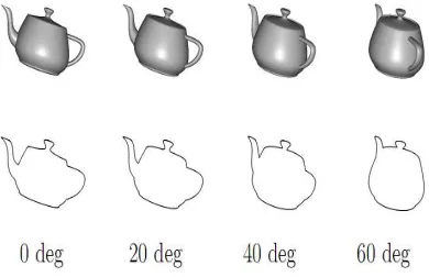
In this experiment, we have used a synthetic Teapot sequence of 18 exact silhouettes shown in Fig. 7. We conducted systematic comparisons between the PO described in [8] and of the GA to estimate the focal length f and the rotation axis coordinates (θa, φa). We found that in this case the
[image:6.612.313.522.71.263.2]PO performs better than the GA, as shown by comparison of the convergence histories in Fig. 8. Both the PO and the basic GA converge correctly to the optimal solution. However, the PO converges to the optimal solution more rapidly than the GA.
Figure 7: Some Views Of Synthetic Teapot Sequence With Their Corresponding Exact Silhouettes And Their
Absolute Camera Angles
Figure 8: Comparison Of The Convergence Histories Of PO And GA For Focal Length And Rotation Axis
Estimation.
In the second test we have increased the complexity of the optimization problem, we have taken 9 views spaced of 20 degrees and we have computed the full circular motion (translation direction αt and rotation axis coordinates (θa, φa),
camera angles ∆ωi) by keeping the focal length to
[image:6.612.94.289.467.593.2]its calibrated value. Fig 9 shows the convergence histories for the basic GA and the PO for this case. As shown in Fig 9 the GA converges correctly to the optimal solution while PO has been trapped in local optimal solution due to bad initialization of starting points. It is important to note that there are different implementations of the PO. Although the version applied in this paper fails to find the global maximum, there may be other versions of the PO that can improve the result. Though, seeking the best version of the Powell optimizer is not the intent of this paper.
[image:6.612.314.525.512.689.2]5.2 Comparison between the GA and Hybrid GA-PO
[image:7.612.316.521.72.256.2]To demonstrate the advantage of the hybrid method over the previous one (basic GA), we applied it to recover camera parameters and motion from real silhouettes. In this experiment, we have used the Hannover dinosaur sequence shown in Fig 10. The dinosaur sequence (36 images) is binarized by a segmentation algorithm, and then the contours are extracted from silhouettes using a GVF snake [19].
Figure 10: Same Images Of Hannover Dinosaur Sequence. From Top To Bottom: Color Images, Binarized
Silhouettes And Contours Extracted From Silhouettes.
Table 1 gives the ranges of values for each parameter that we set for this experiment and the estimation of the rotation axis coordinates (θa, φa),
the translation direction αt and the focal length f by
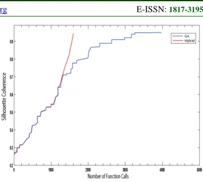
the GA and the Hybrid method. The results are good for both methods. The Hybrid method outperforms the basic GA when computing the rotation axis and the translation direction. The comparison of convergence histories between the both methods is shown in Fig. 11. It is seen that strong improvement is obtained when the PO is launched after 50 generations (1000 function calls). The hybrid method maximizes the CSC faster than
the basic GA.
Table 1: Camera Parameter Estimated By Ga And The Proposed Hybrid Method
Parameters Rotation Translation Focal leght
θa φa αt f
Ground
Truth 92.663 2.261 2.735 3217 Lower range -180 -90 -5 3000
Upper range 180 90 5 3400
Recovered
by GA 92.405 2.272 2.774 3232 Recovered
by Hybrid 92.658 2.257 2.743 3246
Figure 11: Comparison Of The Convergence Histories Of GA And Our Hybrid Method
6 3D MODEL RECOSTRUCTION
The 3D object surface is determined by an octree based algorithm: We dispose of a set of 36 silhouettes (dinosaur sequence in Fig. 10) and their corresponding projection matrices Pi recovered by our hybrid GA-PO method. The algorithm needs two additional input data: the level of detail (the size of the voxel), and an initial bounding box. Starting from the bounding box, the octree approach subdivides a cube into 8 children whenever it is on the isosurface, and iterates the process recursively until the maximum level of depth is attained. To evaluate a given cube, we project it into all the silhouettes to assign it one of the 3 labels [20] depending on whether it lies entirely inside (in), entirely outside (out), or partially intersects the silhouette (on). If the cube is on and the maximum depth is not still reached, we subdivide it and recursively test its children. At the end, only the cubes that are on surface have been subdivided. We can see the result of this step for different levels of resolution in Fig. 13.
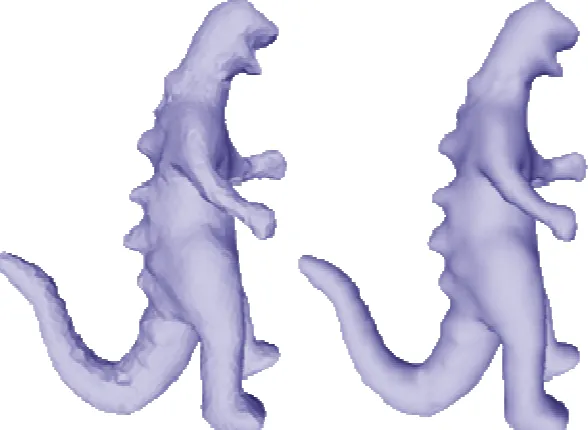
Once the octree is constructed, the next step is to mesh it. Marching cubes algorithm [21] provides an initial consistent surface which is then smoothed using a decimation algorithm. Examples are shown in Fig. 14.
7 CONCLUSION
[image:7.612.91.299.229.366.2]the optimal solution. However, the GA was slower than the PO. Important improvements ware obtained with the hybrid method in term of convergence speed and parameters accuracy. The hybrid method can correctly find the optimal parameters without the need of initial values and successfully avoid to be trapped in local maxima. These characteristics will make the silhouette coherence concept more efficient and powerful to work in general motion instead of circular motion.
ACKNOWLEDGMENT
The dinosaur images used here were provided by Wolfgang Niem at the University of Hannover.
REFRENCES:
[1] R. Hartley and A. Zisserman, Multiple View Geometry, Cambridge University Press, 2000. [2] A. W. Fitzgibbon, G. Cross, and A. Zisserman,
“Automatic 3D model construction for turn-table sequences,” in 3D SMILE, June 1998, pp. 155–170.
[3] G. Jiang, H. Tsui, L. Quan, and A. Zisserman, “Single axis geometry by fitting conics,” in ECCV, vol. 1, 2002, pp. 537–550.
[4] Wong, K.-Y. K. and Cipolla, R. (2001). Structure and motion from silhouettes. In 8th IEEE International Conference on Computer Vision, volume II, pages 217-222, Vancouver, Canada.
[5] Paulo R. S. Mendonca, Kwan-Yee K. Wong, and Roberto Cipolla. Epipolar geometry from profiles under circular motion. IEEE Trans. Pattern Anal. Mach. Intell., 23(6): 604616, 2001.
[6] Carlos Hernndez, Francis Schmitt, and Roberto Cipolla. Silhouette coherence for camera calibration under circular motion. PAMI, 29(2):343349, February 2007.
[7] M. Powell, ”An efficient method for finding the minimum of a function of several variables without calculating derivatives”, Computer Journal, vol. 17, pp. 155162, 1964.
[8] J. H. Holland, Genetic algorithms, Scientif. Am. 44 (1975).
[9] D. E. Goldberg, Genetic Algorithms in Search, Optimization & Machine Learning (Addison-Wesley, Reading, MA, 1989).
[10] A. Mouafi, R. Benslimane, A. El Ouaazizi. A Genetic Algorithm for Recovering Camera Parameters and Motion from Silhouettes. Telecommunications (ICT), 20th International Conference on, 6-8 May 2013.
[11] Matusik, W., Buehler, C., Raskar, R., Gortler, S., and McMillan, L. Image-based visual hulls. SIGGRAPH 2000, pages 369{374.
[12] W. H. Press, S. A. Teukolsky, W. T. Vetterling, and B. P. Flannery, Numerical Recipes, 2nd ed. (Cambrige Univ. Press, Cambridge, UK, 1992). [13] 18. F. S. Acton, Numerical Methods That Work
(Mathematical Association of America, Washington, DC, 1970) p. 464. [1990 corrected edition].
[14] R. P.Brent, in Algorithms for Minimization without Derivatives (Prentice Hall International, Englewood Cliffs, NJ, 1973), Chap. 7.
[15] J. E. Dennis, Jr. and R. B. Schnable, Numerical Methods for Unconstrained Optimization and Nonlinear Equations (Prentice Hall International, Englewood Cliffs, NJ, 1983) [16]Z. Michalewiez,”Genetic Algorithms + Data
Structure = Evolution Programs”, Springer, Berlin, 1992.
[17] A. El ouaazizi, M. Zaim and R. Benslimane, A Genetic Algorithm for Motion Estimation, International Journal of Computer Science and Network Security, VOL.11 No.4, April 2011 [18] A. El ouaazizi, R. Ouremchi and R.
Benslimane, Reconstruction of gray-level image by genetic algorithm , Proceeding of 4th International Conference on Quality Control by Artificial Vision, Japan 1998.
[19] Xu, C. and Prince, J. L. (1998). Snakes, shapes, and gradient vector flow. IEEE Transactions on Image Processing, pages 359-369.
[20] R. Szeliski, Rapid octree construction from image sequence. CVGIP, 58(1):23-32, July 1993.
Figure 13: Octree Generation: The Dinosaur Octree Is Carved From A Single Bounding Box Given 36 Images. From Left To Right: Bounding Box, Level 3, 5, 6 And 7 Of Subdivision.
[image:9.612.162.456.337.552.2]