Computational Fluid Dynamics (CFD) Investigation To Assess Wind Effects On A Tall Structures (Wind Force Parameters)

(1)

COMPUTATIONAL FLUID DYNAMICS (CFD) INVESTIGATION TO ASSESS

WIND EFFECTS ON A TALL STRUCTURES (WIND FORCE PARAMETERS)

G Naga Sulochana

1

_{, H Sarath kumar}

2 1

_{M.Tech Student.}

2

_{Assistant Professor}

1,2

Department of Civil Engineering, AVR & SVR College of Engineering and Technology, Nandyal.

---***---

Abstract

-

The development of high strength concrete,

higher grade steel, new construction techniques and advanced computational technique has resulted in the emergence of a new generation of tall structures that are flexible, low in damping, slender and light in weight. These types of flexible structures are very sensitive to dynamic wind loads and adversely affect the serviceability and occupant comfort. This project presents the results using Computational Fluid Dynamics Technique using Gambit & Fluent software on square building models with an acceptance ratio of 1:1.5:7. The wind force on the models is evaluated from force records obtained from software under Computational Fluid Dynamics Technique using Gambit & Fluent for normal wind directions in a sub-urban terrain conditions for category A.The same rectangle building analyzed manually by IS 875 Part 3: 1987. The value obtained from this are compared with software results. The further study is made for the design and calculation of Gust Response Factor.

Keywords : Windward, Leeward, Guest Response, Acceptance Ratio.

1.INTRODUCTION

Importance Of wind Analysis on Tall Structures:

Wind is air in motion relative to the surface of the earth. The primary cause of wind is traced to earth’s rotation and differences in terrestrial radiation. The radiation effects are primarily responsible for convection either upwards or downwards. The wind generally blows horizontal to the ground at high wind speeds. Since vertical components of atmospheric motion are relatively small, the term ‘wind’ denotes almost exclusively the horizontal wind, vertical winds are always identified as such. The wind speeds are assessed with the aid of anemometers or anemographs which are installed at meteorological observatories at heights generally varying from 10 to30 meters above ground. Very strong winds (greater than 80 km/h ) are generally associated with cyclonic storms, thunderstorms, dust storms or vigorous monsoons. A feature of the. Cyclonic storms over

the Indian area is that they rapidly weaken after crossing the coasts and move as depressions/lows in land. The influence of a severe storm after striking the coast does not, in general exceed about 60 kilometers, though sometimes, it may extend even up to 120 kilometers. Very short duration hurricanes of very high wind speeds called KalBaisaki or Norwesters occur fairly frequently during summer months over east India.

The liability of a building to high wind pressures depends not only upon the geographical location and proximity of other obstructions to air flow but also upon the characteristics of the structure itself

The effect of wind on the structure as a whole is determined by the combined action of external and internal pressures acting upon it. In all cases, the calculated wind loads act normal to the surface to which they apply.

The stability calculations as a whole shall be done considering the combined effect, as well as separate effects of imposed loads and wind loads on vertical surfaces, roofs and other part of the building above general roof level.Buildings shall also be designed with due attention to the effects of wind on the comfort of people inside and outside the building.

2.LITERATURE SURVEY

2.1 Wind Characteristics:.

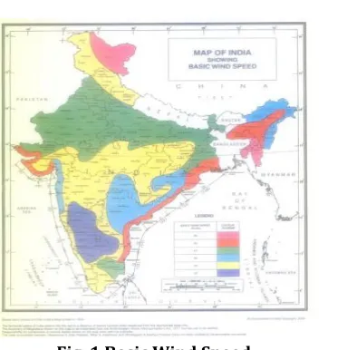
Basic Wind Pressures:

(2)

Fig. 1 Basic Wind Speed

2.2 Gradient Wind Speed:

The gradient wind is a balance of the Pressure Gradient Force, centrifugal and Carioles. A geotropic wind becomes a gradient wind when the wind begins flowing through curved height contours. The curving motion introduces a centrifugal (outward fleeing) force. The centrifugal effect can be felt when turning through a curve in a car. You stay with the car but it feels like you are being pushed sideways.

2.3 Gust Factor:

Only the method of calculating load along wind or drag load by using gust factor method is given in the code since methods for calculating load across-wind or other components are not fully matured for all types of structures. However, it is permissible for a designer to use gust factor method to calculate all components of load on a structure using any available theory. However, such a theory must take into account the random nature of atmospheric wind speed.

2.4Turbulence characteristics

Gustiness occurs due to the velocity fluctuations present in the wind flow and this renders the forces exerted on the structure as dynamic forces. The degree of gustiness is given by standard deviation or RMS velocity value. The turbulent intensity can be obtained from SD and mean velocity and is given in equation.

Iu =( ) or Iu =( )

remains same after gradient height. The variation of wind velocity with time has been illustrated in Fig. 3.3 and is given in equation

Vt = V + V’

Where,

Vt = wind velocity at any given instant of time‘t’

[image:2.612.77.274.89.282.2]

V = average wind V’ = wind gusts

Fig. 2 Variation of wind velocity with time

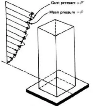
As wind pressures are proportional to the square of velocities, with variation of mean Wind velocity, the mean pressures also fluctuate. The variation of pressure has been shown in Fig.2 and is given by:

Pt = P + P’

Where,

Pt = pressure at any instant of time ‘t’

(3)

Fig 3. Schematic representation of mean and gust pressure at any instant of time‘t’ Along wind and across wind motions

Under the action of wind flow, structure experience aerodynamic forces that include the drag force and lift force. Drag (along-wind) force acting in the direction of the mean wind and the lift (across-wind) force acting perpendicular to that direction. The Along-wind motion primarily results from pressure fluctuations in the windward and the leeward faces, which generally follow the fluctuations in the approach flow. The Across-wind motion is introduced by pressure fluctuations due to vortex shedding in the separated shear layers and wake flow field.

2.5 Wind force F

Along Wind Load - Along wind load on a structure on a strip area ( Ae ) at any height (Z) is given by:

FS = Cf Ae Pz G

where

FS = along wind load on the structure at any height z

corresponding to strip area Ae

Cf = force coefficient for the building,

Ae = effective frontal area considered for the structure at

height Z,

Pz = design pressure at height z due to hourly mean wind

obtained as 0.6 Vz2 (N/m2)

3. Data Collection

Evaluation of wind force

[image:3.612.300.560.92.620.2]

Fig.10 (IS 875-3 Pg.51) shows the different faces of angles considered for the pressure measurement study. The chord length for each face is given as follows: Face A: 0- 10cm, Face B: 10- 25cm, Face C: 25- 35cm, Face D: 35- 50cm

Fig. 4 Forces acting on building

LEVELS Z/H HEIGHT

in cm

Fx1987(00_{) Fy1987(90}0₎

1.000 0.1 7 904 448

2.000 0.2 14 1224 596

3.000 0.3 21 1421 686

4.000 0.5 35 3474 1673

5.000 0.7 49 3874 1859

6.000 0.8 56 2052 984

7.000 0.9 63 2257 1063

8.000 0.95 66.5 1197 586

9.000 1 70 1310 623

[image:3.612.113.210.100.210.2]

1.000 0.1 7 904 448

Table 7 Calculation of force as per IS-875(part-3) 1987 Provisions

Level Leeward (90°) Windward(0°)

[image:3.612.318.555.224.490.2]

(4)

Fig. 5 Forces for manual solutions

4. RESULTS AND DISCUSSION

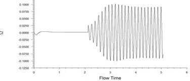
Unsteady numerical simulations have been carried out for a 1:2:5 rectangular building model under uniform wind flow condition using two types of turbulence models available in FLUENT 6.3 software: (i) Realizable k-ε turbulence model, which is single scale type turbulence model and (ii) DES turbulence model with Realizable k-ε option, which is multi-scale type hybrid turbulence model. For the evaluation of pressure coefficients and drag and lift force coefficients, the reference wind velocity is taken as 10 m/s (same as the uniform input wind velocity) and reference area of projected area, i.e. 0.1 m x 0.5 m. Unsteady simulations have been carried out until stabilized mean and standard deviation values of Cd and Cl are obtained with respect to time as shown in Fig.9 in IS 875-3 Pg.50 for Realizable k-ε turbulence model.

[image:4.612.337.525.112.192.2]

A MATLAB program has been developed for processing the numerically simulated Cp values to obtain distributions of mean Cp and standard deviation Cp values at 5 selected levels, viz. 0.05 m, 0.15 m, 0.25 m, 0.35 m, 0.45 m, respectively (correspond to z/H values of 0.1, 0.3, 0.5, 0.7, 0.9 ref. Level 1, Level 2, Level 3, Level 4, Level 5). Further mean Cd and standard deviation Cl values have been at these 5 levels and also for the overall building also. The following sections discuss some these results.

[image:4.612.34.270.129.225.2]

Fig. 6: Variation of drag coefficient with time - Realizable k-ε turbulence model

Fig 7: Variation of lift coefficient with time - Realizable k-ε turbulence model

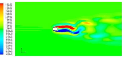
Velocity Vector Plots

Figs. 6 and 7 show the velocity vector plot on center vertical plane for Realizable k-ε case. It can be seen over the roof of building significant increase in wind velocity due to separation from the windward edge of the roof. Further in the wake region, i.e. rear side of the building, flow with recirculation is observed with wind in opposite direction along with vertical wind near to building rear side Fig.10 in IS 875-3 Pg.51 shows the velocity vector plot for DES case. Unlike for Realizable k- ε case, it Can be seen multiple eddies in the wake region of the building, which is due to DES model can simulate multi-scale turbulence, i.e. eddies with different sizes.

Fig. 8: Velocity vector plot on center vertical plane – Realizable k- ε turbulence model

[image:4.612.326.541.572.675.2] [image:4.612.40.238.590.678.2]

(5)

Fig. 10 Velocity vector plot on center vertical plane – DES turbulence model

Vorticity Contours

[image:5.612.327.540.431.537.2]

Vorticity is a measure of the rotation of a fluid element as it moves in the flow field and is defined as the curl of the velocity vector. It is show the vorticity contour plots in horizontal plane at Level 1, Level 3 and Level 5, respectively for Realizable k-ε turbulence model. It can be seen that the vortex shedding is predominant at Level 1 and as the height of the level increases, the vortex shedding phenomenon is observed to be affected. This is due to the wind flow from the top of the building into the wake region affecting the vortex shedding in the top region of the wake. SimilarlyFig.9 in IS 875-3 Pg.50show the vorticity contour plots in horizontal plane at Level 1, Level 3 and Level 5, respectively for DES turbulence model. Similar to Realizable k-ε predictions, the vortex shedding phenomenon is observed to be affected in the top region of the wake. However, DES predictions show vortex shedding with multiple eddies in the wake region.

Fig. 11 Vorticity Contour in horizontal plane at Level 1 – Realizable k-ε turbulence model

Fig. 12 Vorticity Contour in horizontal plane at Level 3 – Realizable k-ε turbulence model

[image:5.612.38.253.470.570.2]

Fig. 13 Vortices Contour in horizontal plane at Level 5 – Realizable k-ε turbulence model

Fig. 14 Vorticity Contour in horizontal plane at Level 1 – DES turbulence model

[image:5.612.323.541.580.678.2]

(6)

[image:6.612.330.568.88.302.2]

Fig. 16 Vorticity Contour in horizontal plane at Level 5– DES turbulence model Mean Cp Distributions

Fig.10 in IS 875-3 Pg.51 show the mean Cp contour on the rectangular building obtained using Realizable k-ε and DES turbulence models, respectively. It can be seen that on the front face, the mean Cp variation along the height is observed to be mostly uniform except at top and bottom regions, where the edge effects are expected. On the back face, the mean Cp values are observed to be negative, i.e

suction pressure and their magnitudes are observed to be increasing with increase in height. However, on the side faces, difference in the mean Cp distributions is observed between the two turbulence models.

Further, mean Cp distributions along the circumference of the building at 5 levels, viz. Level 1, 2, 3, 4 and 5, have been shown in Fig.10 in IS 875-3 Pg.51 based on the Realizable k-ε and DES turbulence models, respectively. It can be seen that for both the turbulence models, on the front face, the mean Cp values are almost same for Levels 2, 3 and 4, whereas at Levels 1 and 5, the mean Cp values are less. On the back face, in general, the mean Cp suction magnitudes are observed to be increasing with increase in height. On the side face, the mean Cp values are observed to be same for all the levels except for Level 1 in the case of Realizable k-ε turbulence model .

Fig.10 in IS 875-3 Pg.51 show the distribution of mean Cp along the circumference for levels 1, 3 and 5, respectively, to study the difference between the predictions of Realizable k-ε and DES turbulence models. It can be seen that on the front face both the turbulence models predict almost same mean Cp values. However, the mean Cp suction magnitudes on the side and back faces are observed to be more in the case of DES turbulence model than those in the case of Realizable k-ε turbulence model. At Level 1, Realizable k-ε turbulence model is observed to predict pressure recovery on the side faces from the windward edge. At Level 5, the mean Cp distribution along the side and back faces are observed to be nearly uniform based on both the turbulence models.

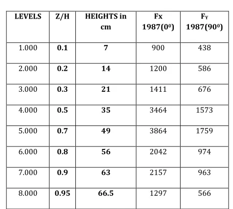
5.000 0.7 49 3864 1759

6.000 0.8 56 2042 974

7.000 0.9 63 2157 963

[image:6.612.37.261.96.200.2] [image:6.612.343.559.357.473.2]

8.000 0.95 66.5 1297 566

Table 7 Calculation of force as per IS-875(part-3) 1987 Provisions

Level Leeward (90°) Windward(0°)

[image:6.612.325.564.497.648.2]

1.000 900 438 2.000 1200 586 3.000 1411 676 4.000 3464 1573 5.000 3864 1759 6.000 2042 974 7.000 2157 963 8.000 1297 566 9.000 622.840 1310.187

(7)

[image:7.612.53.272.120.288.2]

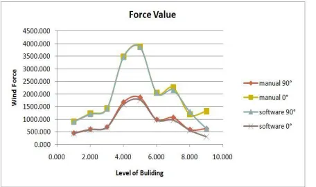
Fig. 17: Forces for software solutions

manual

90° manual 0° software 90° software 0°

[image:7.612.37.265.323.458.2]

1.000 447.813 904.415 900 438 2.000 596.178 1224.411 1200 586 3.000 686.036 1420.865 1411 676 4.000 1673.259 3473.529 3464 1573 5.000 1859.123 3874.313 3864 1759 6.000 983.512 2052.260 2042 974 7.000 1062.681 2256.651 2157 963 8.000 585.652 1196.696 1297 566 9.000 622.840 1310.187 632.840 310.187

Table 7 Comparison of force for both manual and soft ware solutions

Fig. 18 Comparison of force for both manual and soft ware solutions

5. CONCLUSIONS

Mean force value for 00_{for Level 5 is always higher than all}

the other levels due to greater area of projection and edge effect at the ground level. For all other levels, values are almost same with draft code and IS: 875 (part-3) 1987 which indicates that these values are mostly governed by buffeting characteristics of approaching wind flow.

Mean force value for 00_{for Level 5 is always higher than all}

the other levels due to greater area of projection and edge effect at the ground level. For all other levels, values are greater than with draft code and IS: 875 (part-3) 1987 of 0.2 ratio which indicates that these values are not governed by buffeting characteristics of approaching wind flow.

Standard deviation of force coefficients shows decrease in value with height which shows that these parameters depend on the decrease in turbulence intensity with height.

The mean value of drag and lift coefficients obtained from IS: 875 are 2.0547 and 1.9287 and Draft code value obtained 2.1994 and 2.1809 and experimental value obtained is 2.0374 and 1.7845, which is in good agreement with code values for 00 _{but for 90}0_{, these values are differing this is due}

to Wake Effect.

The value of force obtained from IS 875 Part 3 447.813 for 900_{it is the drag coefficient and 900 for 90}0_{with Gambit and}

Fuent. This variation is due to vertex shedding at all levels.

6. REFERENCES

1. Alexandre Luis Braun and Armando Miguel Awruch, 2009. Aerodynamic and aeroelastic analyses on the CAARC standard tall building model using numerical simulation. Computers and Structures, 87, 564–581

2. Huang M.F., HLau I.W., Chan C.M., Kwok K.C.S. and G.Li, 2011. A hybrid RANS and kinematic simulation of wind load effects on full-scale tall buildings. Journal Wind Eng. Ind. Aerodyn, 99, 1126–1138.

3. Shenghong Huanga, Lib Q.S. and Shengli Xua, 2007. Numerical evaluation of wind effects on a tall steel building by CFD. Journal of Constructional Steel Research, 63, 612– 627.

4. Claudio Mannini, Ante Soda and Gunter Schewe, 2011. Numerical investigation on the three-dimensional unsteady flow past a 5:1 rectangular cylinder. Journal Wind Eng. Ind. Aerodyn, 99, 469–482.

5. S. M. Fraser and C. Carey, 1990. Numerical and experimental analysis of flow around isolated and shielded cubes. Appl. Math. Modelling, 14, 588-597.

6. Bosch G. and Rodi W., 1998. Simulation of vortex shedding past a square cylinder with different turbulence models. International Journal for Numerical Methods in Fluids. 28, 601–616.

7. Kimura I. and Hosoda T., 2003. A non-linear k-ԑ model with realizability for prediction of flows around bluff bodies. International Journal for Numerical methods in fluids. 42, 813–837.

(8)