The role of diffusion on the interface
thickness in a ventilated filling box
Kaye, N, Flynn, M, Cook, M and Ji, Y
http://dx.doi.org/10.1017/S0022112010000881
Title
The role of diffusion on the interface thickness in a ventilated filling box
Authors
Kaye, N, Flynn, M, Cook, M and Ji, Y
Type
Article
URL
This version is available at: http://usir.salford.ac.uk/11431/
Published Date
2010
USIR is a digital collection of the research output of the University of Salford. Where copyright
permits, full text material held in the repository is made freely available online and can be read,
downloaded and copied for noncommercial private study or research purposes. Please check the
manuscript for any further copyright restrictions.
doi:10.1017/S0022112010000881
The role of diffusion on the interface thickness
in a ventilated filling box
N. B. K A Y E1, M. R. F L Y N N2†, M. J. C O O K3 A N D Y. J I4
1Department of Civil Engineering, Clemson University, Clemson, SC 29634, USA 2Department of Mechanical Engineering, University of Alberta, Edmonton, AB, Canada T6G 2G8
3Department of Civil and Building Engineering, Loughborough University,
Leicestershire LE11 3TU, UK
4Institute of Energy and Sustainable Development, De Montfort University,
The Gateway, Leicester LE1 9BH, UK
(Received13 October 2009; revised 10 February 2010; accepted 11 February 2010; first published online 9 April 2010)
We examine the role of diffusivity, whether molecular or turbulent, on the steady-state stratification in a ventilated filling box. The buoyancy-driven displacement ventilation model of Linden et al. (J. Fluid Mech., vol. 212, 1990, p. 309) predicts the formation of a two-layer stratification when a single plume is introduced into an enclosure with vents at the top and bottom. The model assumes that diffusion plays no role in the development of the ambient buoyancy stratification: diffusion is a slow process and the entrainment of ambient fluid into the plume from the diffuse interface will act to thin the interface resulting in a near discontinuity of density between the upper and lower layers. This prediction has been corroborated by small-scale salt bath experiments; however, full-scale measurements in ventilated rooms and complementary numerical simulations suggest an interface that is not sharp but rather smeared out over a finite thickness. For a given plume buoyancy flux, as the cross-sectional area of the enclosure increases the volume of fluid that must be entrained by the plume to maintain a sharp interface also increases. Therefore the balance between the diffusive thickening of the interface and plume-driven thinning favours a thicker interface. Conversely, the interface thickness decreases with increasing source buoyancy flux, although the dependence is relatively weak. Our analysis presents two models for predicting the interface thickness as a function of the enclosure height, base area, composite vent area, plume buoyancy flux and buoyancy diffusivity. Model results are compared with interface thickness measurements based on previously reported data. Positive qualitative and quantitative agreement is observed.
1. Introduction
The filling box model, first proposed by Baines & Turner (1969), provides a prediction for the buoyancy distribution in a sealed enclosure with a single-point source of buoyancy. The model has been applied to mixing in the atmosphere and ocean (Baines & Turner 1969; Manins 1979), magma chambers (Huppertet al.1986) and liquid natural gas storage tanks (Germeles 1975). In the filling box analysis, a buoyancy source located in the centre of the enclosure floor creates a plume that rises to the top of the space and forms an expanding buoyant upper layer that is
L L
Q
h H
F0
[image:3.493.154.353.47.177.2]g(z)
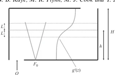
Figure 1. A ventilated filling box, of total heightH, with a nominal interface heighthand an interface thickness 2L.
separated from the lower ambient layer by a sharp density interface or ‘first front’. Baines and Turner’s model (Baines & Turner 1969) was subsequently extended by Linden, Lane-Serff & Smeed (1990) to consider an enclosure connected by upper and lower vents to an extensive external environment, applicable in describing natural ventilation airflows in buildings. In a ventilated filling box, the presence of the upper buoyant layer creates a pressure difference across the vents, which in turn drives a draining flow. Steady state is realized when this draining flow is balanced by the convective plume flow.
In the models described above, diffusive processes are regarded as slow and molecular transport is therefore ignored. Further, observations of small-scale laboratory experiments show interface thicknesses of less than 1 mm, appearing to confirm the no diffusion assumption. However, just as there is a balance between the draining and filling flows in a ventilated filling box, there is also a balance between the rate at which the interface spreads by diffusion and thins by entrainment into the plume. This paper explores the conditions under which diffusion is important.
Firstly, we consider the time scales relevant to a ventilated filling box flow, as depicted schematically in figure 1. The transient model for a single enclosure was presented by Kaye & Hunt (2004). They demonstrated that the time evolution is controlled by the magnitude of the emptying time
Te=
C1/2AH4/3
AF1/3
0
≡ A
A
H gp|z=H
1/2
(1.1)
relative to the filling time
Tf = A
CF01/3H2/3 . (1.2)
Here Te is proportional to the amount of time required for buoyant fluid to drain from a ventilated box after the cessation of convective forcing. Conversely, Tf is proportional to the amount of time required for a closed box to fill with buoyant fluid. In the above equations,A is the floor area,H is the enclosure height andA is the composite effective vent area defined as
A = 2
1/2A
TAB (A2
T+A2B)1/2 ,
constant in which α 0.1 is the entrainment coefficient for an axisymmetric, ‘top hat’ plume. Finally, F0 is the plume source buoyancy flux,zis the vertical coordinate
measured from the floor andgp is the plume-reduced gravity. For ideal plumes whose source volume flux,Q0, is vanishingly small,gp|z=H =C−1F
2/3
0 H−5/3(Baines & Turner
1969). Because the terminal interface height is controlled by the balance of the filling and emptying processes, it too must be a function of Tf andTe, or more specifically their ratio
Tf Te
= A
H2C3/2 . (1.3)
Including diffusive effects through a transport coefficient,κ, adds an additional time scale to the problem, namely the time taken for buoyancy to diffuse over the depth of the enclosure
Tκ = H2
κ . (1.4)
The interface thickness, 2L, is controlled by a balance between diffusion and entrainment and therefore depends on the following ratio of the diffusion and filling time scales:
Tκ Tf
= CF
1/3 0 H8/3
κA . (1.5)
Formally, and for reasons that will become clear in§2.2, it is advantageous to multiply the above ratio by (2α)4/3C−1and thereby define a non-dimensional parameterRsuch
that
R ≡ (2α)4/3
C ·
Tκ Tf
= (2α)
4/3F1/3 0 H8
/3
κA , (1.6)
where R is a ratio relating the rate of convection to diffusion, similar to the P´eclet number Pe, which is a ratio relating the rate of advection to diffusion.
For R 1, diffusion plays only a minor role and a relatively thin interface is anticipated. This is typically the case for similitude experiments of full-scale ventilation flows. In a typical experiment, H 30 cm,A30 cm×20 cm andF0 250 cm4 s−3
(see e.g. Lin & Linden 2002). Selecting the molecular value for the diffusion coefficient appropriate for salt in water yields R 7.5×10⁵. A smaller, possibly significantly
smaller, value for R would be obtained if one chose an eddy, rather than the molecular, diffusivity. However, the magnitude of the eddy diffusivity depends upon the flow and entrainment characteristics inside the particular experimental apparatus; detailed information of this type is typically not recorded or reported in similitude experimental modelling. Conversely, in a full-scale ventilation flow, we consider F0
5.4×10⁻³m4 s−3, corresponding to a 10◦C temperature difference between the source and the surroundings and a source flow rate of 1 air change per hour for a room of dimensions 3 m tall by 20 m2 plan area. Selecting again a value for κ based on
molecular diffusion, in this case for heat through air, givesR 9.2×10², roughly 103
In §2, we present a first-order phenomenological model that balances the rate of thickening of the interface due to diffusion with the rate of thinning due to entrainment into the plume. Also discussed are the integral plume equations that describe a ventilated filling box. Results are contrasted against measured CFD and experimental data as reported in earlier investigations; this discussion appears in§3. Finally, in§4, a series of conclusions are drawn.
2. Role of diffusion
2.1. Approximate solution
We begin with the standard solution to the one-dimensional diffusion equation for an initial step change in the concentrationΥ of an active scalar, say heat or salt:
Υ(z, t) = Υ0 2
1 + erf
z (4κt)1/2
. (2.1)
At arbitrary timet, the interface can be regarded as having diffused a distance
L∼(4κt)1/2. (2.2)
Alternatively, we can regard the diffusion front as a front moving with velocity
u= dL dt =
2κ
L (2.3)
relative to the stationary terminal interface height.
Now consider a ventilated enclosure with an initially sharp interface at height h. Over time the (two-sided) interface will grow in volume with a time rate of change given by
(Q)diffusion = 2A
dL dt =
4κA
L . (2.4)
In addition, buoyant fluid enters the bottom of the diffuse layer and is extracted from the top via the plume. Ignoring stratification effects (This omission is justified
a-posteriori by the results of figure 3), and assuming that the rising flow remains in pure plume balance, the plume volume flux is given byQ=CF01/3(z+z0)5/3 (Woods,
Caulfield & Phillips 2003). Here z0 = [Q0/(CF01/3)]3/5 is the distance of the virtual
source below the actual source. The net rate at which fluid is extracted from the diffuse interface is therefore
(Q)entrainment =CF1
/3 0
(h+z0+L)5/3−(h+z0−L)5/3
. (2.5)
Balancing the rates of diffusion and entrainment yields
4κA
L =CF
1/3 0
(h+z0+L)5/3−(h+z0−L)5/3
⇔ 1 R = 3 20 9 20
1/3 π2/3L
H
ζss+ζ0+
L H
5/3 −
ζss+ζ0−
L H
5/3
, (2.6)
where ζss = h/H and ζ0 = z0/H. Physical insights into the solution structure can
0.02 0.04 1 2 3 0 0.5 1.0
A*/H2 A*/H2
(a) (b)
log10R log10R
[image:6.493.56.427.58.196.2]ζ = z / H 0.02 0.04 1 2 3 0 0.5 1.0
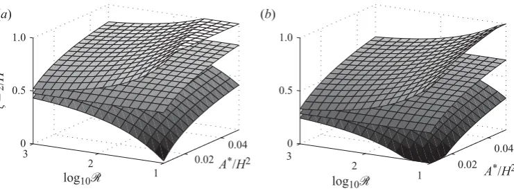
Figure 2. (a) Ideal plume: normalized interface height as a function of A∗/H2 (middle surface) as determined from (2.9). Surfaces showing the thickness of the diffuse interface are also presented; these are based upon the solution to (2.6) withζ0 = 0. (b) Non-ideal plume: as in (a) but withζ0= 0.25. The interface height is now determined by solving (2.10).
L/H ζss+ζ0, the leading-order solution is given by
L
6κA 5CF01/3(h+z0)2/3
1/2
⇔ L
H
2
R
1/2
2×51/2
3π(ζss+ζ0)
1/3
. (2.7)
In the opposite limit, i.e.L/H ζss+ζ0,
L 2κA
CF01/3
3/8
⇔ L
H
20 9π2
1/8
10 3R
3/8
. (2.8)
Here the interface is both thick and close to the floor; the small parameters ζss and ζ0 do not appear in (2.8). Consistent with Baines (1983), (2.7) and (2.8) indicate that
the interface thickness, 2L, grows with increasing floor area and diffusion coefficient. By contrast, 2Lwill be relatively small for larger plume buoyancy fluxes.
The connection between (2.6) and the chamber geometry and source conditions is elucidated as follows: when the plume is ideal i.e.Q0 = 0,ζss, can be determined from
A H2 =C
3/2
ζ5
ss 1−ζss
1/2
(2.9)
(Linden et al. 1990). When the source is non-ideal and AT =AB, ζss is determined instead from (Woods et al.2003)
A H2 =
C3/2(ζ
ss+ζ0)5/6
(1−ζss)1/2
(ζss+ζ0)10/3+ 12ζ10
/3 0 −ζ
5/3
0 (ζss+ζ0)5/3
1/2
. (2.10)
In figure 2, we consider solutions to (2.6), (2.9) and (2.10) for a range ofA∗/H2 and
Rand a pair of values forζ0.
2.2. Ventilated filling box model
buoyancy flux,πF; the latter equation specifies the spatial-temporal variation of the reduced gravityg≡g(ρa−ρ¯p)/ρ00. Hereρ00 is a reference density,ρa is the ambient density and ¯ρp is the horizontal-average plume density. Using subscripts to indicate differentiation with respect to the vertical coordinatezand timet, the equations read (see e.g. Germeles 1975; Manins 1979)
Qz= 2αM1/2, Mz= QF
M , (2.11a, b)
Fz=−Qgz, gt+
Qv−πQ
A g
z=κgzz. (2.12a, b)
In the above, the advection velocity of (2.12b) is equal to the background ambient velocity, which is itself proportional to the difference between the ventilation flow rate Qv and the local plume volume fluxπQ.
With the notable exception of Manins (1979), many previous investigations follow the assumptions applied by Baines & Turner (1969) whereby diffusion is omitted and gt tends to a constant in the long-time limit. Herein, we return to Manins’s approach, albeit in a ventilated rather than a closed filling box, and instead consider steady solutions with a non-vanishing diffusion coefficient. Non-dimensional variables are introduced such that
g= F
2/3 0 δ
(2α)4/3H5/3, z=H ζ , F =F0f , (2.13a, b, c)
Q= (2α)4/3F1/3 0 H5
/3q , M = (2α)2/3F2/3 0 H4
/3m . (2.14a, b)
Applying (2.13) and (2.14) in (2.11) and (2.12) withgt →0 yields
qζ =m1/2, mζ = qf
m , (2.15a, b)
fζ =−qδζ, γζ =Rγ(qv−πq), δζ =γ , (2.16a, b, c) where R, whose magnitude dictates the stiffness of the above system of ordinary differential equations, is defined by (1.6) and the second-order equation (2.12b) has been broken into the two first-order equations (2.16b,c).
Boundary conditions appropriate to the case of an ideal plume are q(0) = 0, m(0) = 0, f(0) = 1 and δ(0) = 0. The numerical value of γ(0) is selected such that f(1) = 0, i.e. the plume buoyancy flux at the top of the chamber vanishes. Unless the interface naturally lies close to the upper boundary and/orR∼ O< (101) such that the
interface is especially broad, f(1) = 0 ⇒δ(1) =π/qv ⇔g(H) = πF /Qv, the latter condition being consistent with the analysis of Linden et al. (1990). When solving the system of ordinary differential equations, a pair of iterations are necessary. For prescribed qv and from a pair of sensible initial guesses for γ(0) (>0), we converge to that unique value of γ(0) satisfying f(1) = 0. Then, by integrating δ with height, the actual non-dimensional ventilation flow rate may be evaluated from (cf. (2.15) of Lindenet al.1990)
qv = 1 4α2
A H2
1
0
δdζ
1/2
⇔
Qv A
2
=
H
0
gdz. (2.17)
The original estimate forqvis updated accordingly and we repeat the above steps until a tolerance of 1×10⁻⁷ onq
−0.20 0 0.2 0.4 0.6 0.8 1.0 1.2 0.2
0.4 0.6 0.8 1.0
q, m, f
[image:8.493.143.334.61.217.2]ζ
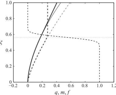
Figure 3. Solutions to the (diffusive) filling box equations (2.15)–(2.16) with
A/H2 = 1.41×10⁻², R= 500 and ζ
0 = 0. The dashed and thick solid and dash-dotted lines show, respectively, f,q andm. The thin solid and dash-dotted lines are described in the text and the thin horizontal line shows the vertical location,ζ = 0.564, whereq=qv/π.
solution behaviour is then governed by the pair of non-dimensional parameters R andA/H2. Whereas a formal investigation of the convergence characteristics for the
above algorithm is deferred to a future investigation, we note in passing that the present approach is largely successful providedR∼< 103–104 (i.e. the system stiffness
is allowed to be large but not extreme) and the centre of the interface (i.e. the location whereπq =qv and, from (2.16b) and (2.16c), whereδζ attains its maximum value) is not too close to the upper boundary.
Representative output for a particular combination of A/H2 and R is given in
figure 3. It shows vertical profiles of q, m and f as determined from (2.15a), (2.15b) and (2.16a), respectively. Outside of the interfacial region, the buoyancy flux is nearly constant, either f 1 in the lower layer or f 0 in the upper layer. Because f
becomes vanishingly small asζ tends to 1,m(denoted by the thick dash-dotted line) approaches a constant value and q(denoted by the thick solid line) becomes a linear function of height. For reference, the thin solid and dash-dotted lines of figure 3 show, respectively, vertical profiles of q and mfor the special case of an unstratified ambient with f(ζ) = 1. The deviation between the thick and thin dash-dotted lines begins abruptly near the vertical location where πq and qv coincide. Conversely, the thick and thin solid lines do not deviate significantly from one another except relatively close to the top of the enclosure, i.e. ζ ∼> 0.7. Note that exact solutions may be derived when f(ζ) = 1 (Morton, Taylor & Turner 1956) and have the form q = (3/5) (9/20)1/3ζ5/3, m= (9/20)2/3ζ4/3.
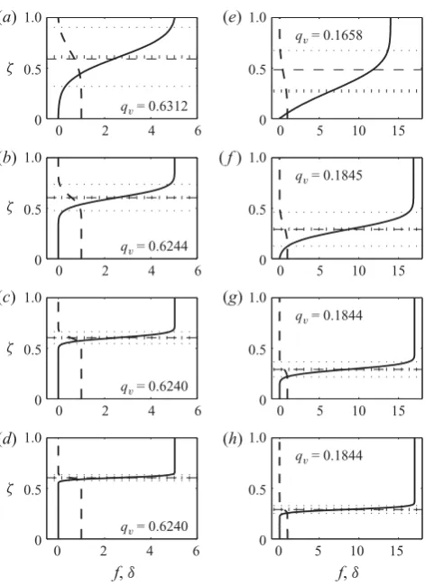
Further solutions to the (diffusive) filling box equations are presented in figure 4, which considers two different values of A/H2, and R spanning two orders of
0 5 10 15 qv = 0.1658
0 5 10 15
qv = 0.1845
0 5 10 15
qv = 0.1844
0 5 10 15
qv = 0.1844
0 2 4 6
0 0.5 1.0
(a) (e)
(b) (f)
(c) (g)
(d) (h)
qv = 0.6312
0 2 4 6
0 0.5 1.0
qv = 0.6244
0 2 4 6
0 0.5 1.0
qv = 0.6240
0 2 4 6
0 0.5 1.0
0 0.5 1.0
0 0.5 1.0
0 0.5 1.0
0 0.5 1.0
f, δ f, δ
qv = 0.6240 ζ
ζ
ζ
[image:9.493.137.373.57.382.2]ζ
Figure 4.Vertical distributions of f (dashed line) and δ (solid line) for ζ0 = 0,
A/H2 = 1.77×10⁻² (a–d),A/H2= 2.12×10⁻³ (e–h) and (a, e) R= 20, (b, f) R= 100, (c, g)R= 500 and (d,h)R= 2×10³. The middle dotted horizontal line (thick) shows the point at which q = qv/π and the upper and lower dotted horizontal lines (thin) indicate the interfacial thickness based on the estimate of (2.6). The dashed horizontal line shows the equivalent interface height assuming an upper layer of uniform buoyancy withδ=π/qv.
3. Comparison with previous analyses
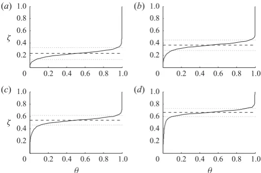
For most cases of architectural interest, and consistent with figure 4, (2.7) is the more relevant approximation to (2.6) than (2.8). Here, we contrast the thin interface approximation (2.7) with previously published measurements of buoyancy profiles in model ventilated enclosures. A representative set of scaled temperature profiles from Kaye, Ji & Cook (2009) is shown in figure 5 along with the interface height predicted from Lindenet al.(1990) and the upper and lower bounds on the interface thickness predicted from (2.7). Positive agreement between the simple scaling model and the full simulation results is observed suggesting that diffusion is the primary cause of interfacial thickening.
0 0.2 0.4 0.6 0.8 1.0
0 0.2 0.4 0.6 0.8 1.0
0.2 0.4 0.6 0.8 1.0 0.2 0.4 0.6 0.8 1.0
0.2 0.4 0.6 0.8 1.0 0.2 0.4 0.6 0.8 1.0
0 0.2 0.4 0.6 0.8 1.0
0 0.2 0.4 0.6 0.8 1.0
(a) (b)
(c) (d)
ζ
ζ
[image:10.493.106.372.60.236.2]θ θ
Figure 5. Scaled temperature profiles, θ = (T −Tf loor)/(Tceiling−Tf loor), plotted against ζ, based on the CFD simulations of Kayeet al.(2009), with the interface limits predicted by (2.7) indicated by the horizontal dotted lines. The horizontal dashed lines show the interface height predicted by Lindenet al.(1990). (a)A/H2= 0.0026, (b)A/H2= 0.0078 (c)A/H2= 0.0208 and (d)A/H2= 0.0624.
Quantitative comparison with full scale results is problematic due to a lack of published data regarding the detailed vertical temperature profile in a full-scale room with well-categorized heat inputs. One might argue that the near full-scale data of Howell & Potts (2002) could suffice. However, in Howell & Potts’s experiments, calculations based on their published data and standard heat transfer correlations show that their heat source had an operating temperature of approximately 165◦C. This is significantly hotter than typical surfaces in most commercial buildings indicating that the collected data may be unduly influenced by radiative and non-Boussinesq effects. As such, there are different, and more complicated, heat transfer effects that come into play in interpreting Howell and Potts’ measured results (Howell & Potts 2002), making a straightforward comparison to the present models nontrivial. Even so, it is worth pointing out the qualitative similarities between the vertical buoyancy profiles of figures 3, 5, 8 and 9 from their paper and the solid curves of figure 4 (e, f). Whereas Howell & Potts (2002) suggest that radiative effects must be incorporated in order to generate buoyancy profiles of such a distinctive shape (i.e. nearly linearly stratified through the lower layer with a uniform temperature in the upper layer), our analysis demonstrates that diffusive effects alone suffice. In a similar vein, Howell and Potts’ criticisms of the two-layer model of Linden
4. Discussion and conclusions
Filling box models such as that first proposed by Baines & Turner (1969) have been broadly applied in describing isolated convection in closed and ventilated geometries. Consistent with their analogue salt-bath experiments, Baines and Turner’s equations neglect diffusion so that there is a discontinuous density jump across the ‘first front’, the interface that separates the uncontaminated ambient from the fluid that previously originated from, or was entrained into, the plume. While this modelling approach can accurately predict, among other quantities, the ventilation flow rate (Lindenet al.
1990), it may fail to reproduce the distributed vertical temperature profiles that are often noted, for example, in full-scale measurements of naturally ventilated buildings (Howell & Potts 2002).
From phenomenological arguments, we give via (2.6) and its approximates equations for the interface thickness as a function of the diffusion and entrainment coefficients, respectively, κ and α; the plan area of the enclosureA; the chamber heightH; the source volume and buoyancy fluxes; and the area of the openings that connect the enclosure to a much more voluminous ambient. Model predictions are corroborated by solving the filling box equations, (2.15) and (2.16), where, as with the earlier analysis of Manins (1979),κis assumed to be non-zero. In both cases, the interface thickness is predicted to be a decreasing function ofR, defined by (1.6), which is analogous to the P´eclet number, Pe. Comparisons are also drawn against related measurements from previous CFD, experimental and full-scale analyses as summarized in§3. Generally positive agreement is noted.
Viewed from a different perspective, (2.6) or the (diffusive) filling box equations may be applied in estimating a representative ambient diffusion coefficient κ in architectural or environmental instances where source conditions and a vertical gradient of temperature are well known. Such an approach has the benefit of simplicity since detailed microstructure measurements are not required, albeit at the expense of providing average rather than spatially detailed predictions for the eddy diffusion coefficient.
Financial support was generously provided by Clemson University and NSERC through the Discovery Grant programme. The helpful comments of three anonymous referees are acknowledged with thanks.
R E F E R E N C E S
Baines, W. D.1983 Direct measurement of volume flux of a plume.J. Fluid Mech.132, 247–256. Baines, W. D. & Turner, J. S. 1969 Turbulent buoyant convection from a source in a confined
region.J. Fluid Mech.37, 51–80.
Germeles, A. E.1975 Forced plumes and mixing of liquids in tanks.J. Fluid Mech.71, 601–623. Howell, S. A. & Potts, I.2002 On the natural displacement flow through a full-scale enclosure
and the importance of the radiative participation of the water vapour content of the ambient air.Build. Environ.37, 817–823.
Huppert, H. E., Sparks, R. S. J., Whitehead, J. A. & Hallworth, M. A.1986 Replenishment of magma chambers by light inputs.J. Geophys. Res.91, 6113–6122.
Kaye, N. B. & Hunt, G. R.2004 Time-dependent flows in an emptying filling box.J. Fluid Mech.
520, 135–156.
Kaye, N. B., Ji, Y. & Cook, M. J.2009 Numerical simulation of transient flow development in a naturally ventilated room.Build. Environ.44, 889–897.
Linden, P. F., Lane-Serff, G. F. & Smeed, D. A.1990 Emptying filling boxes: the fluid mechanics of natural ventilation.J. Fluid Mech.212, 309–335.
Manins, P. C.1979 Turbulent buoyant convection from a source in a confined region.J. Fluid Mech.
91, 765–781.
Morton, B. R., Taylor, G. I. & Turner, J. S. 1956 Turbulent gravitational convection from maintained and instantaneous sources.Proc. R. Soc. A234, 1–23.