2018 3rd International Conference on Computational Modeling, Simulation and Applied Mathematics (CMSAM 2018) ISBN: 978-1-60595-035-8
The Distribution of the Sum of Independent Generalized
Gaussian Signals
Tai-yue WANG
*and Yan-qing DAI
School of Mathematics and Physics, Hubei Polytechnic University, Huangshi, 435003, P. R. China
*Corresponding author
Keywords: Generalized Gaussian distribution, High order statistics, Gaussian signal.
Abstract. The distribution of the sum of independent generalized Gaussian signals is studied in the paper. The properties of the sum of signals in detail are firstly analyzed. The conclusion that the distribution of the sum of generalized Gaussian signals is not generalized Gaussian distribution was obtained; the reasoning for the special case is given to support the proposed conclusion. The simulation results show that applying generalized Gaussian distribution to model the distribution of the sum based on high order statistics, they coincide with each other well except for the vicinity of mean.
Introduction
Generalized Gaussian Distribution(GGD) has a symmetric unimodal density characteristic with variable tail length and contains the Laplacian, Gaussian and uniform distributions as special cases. Therefore, GGD can be used to describe many kinds of noise [1-3], and to model the Probability
Density Function(PDF) of transform and subband coefficients such as DCT[4] and DWT[5-6]
coefficients. So, the signals with generalized Gaussian distribution (GGD) became the research hotspot in the field of signal processing and information security in recent years. Sometimes the sum of independent generalized Gaussian signals need be studied, or the linear system driven by
generalized Gaussian white noise, whose PDF is approximated by PDFof generalized Gaussian [7]. It
is well known the GGD has analytical expression for its probability density function. However, our research shows such is not the case for the sum of independent GG signals. The paper will show that the sum of independent GG signals is no longer GGD, and a new distribution similar to GGD.
Generalized Gaussian Distribution
A detailed treatment of GGD can be found in[8]. The generalized Gaussian PDF[9] is given by
( ; , , ) exp
2 (1 )
x
f x x R
(1)
where 1
0
( )z e t dtt z
,) 3 (
) 1 (
2
, and , ,2 are mean, shape parameter and variance
respectively. The shape parameter0determines the rate of exponential decay of the PDF. Note
[image:1.595.198.383.686.768.2]that for2, the density reduces to the Gaussian density, whereas for1it becomes the Laplacian density. Some members of the class are illustrated in Figure 1 for =0, =10,= 0.7,1,2 and 100.
Based on the PDF of GGD in (1), we can characterize some of the properties as follows.
(1.a) Symmetry f(x) f(x); (2.a) Monotonicity The PDF is strictly monotone increasing forx, strictly monotone decreasing forx, and reaches the maximum forx.
(3.a) Convexity Since 2 1
2
2 (1 )
( ) exp x ( 1)
f x x x
,it is obvious
that
if f x( )0 1,for any x; If 1, f x ( ) 0, for x
1 1
1
and f x( )0 for
1
1 1
x .
(4.a) ( )
1
2 ( )
f
, (5.a) Due to the symmetry of the PDF in(1), the odd moments
2 1
X k
E vanish,
where X is with zero mean. The even moments are given as follows
2 2 (2 1 )
X
(1 )
k k k
E
(2)
(6.a)Eq.(2) and the cumulant properties[10] give the nth-order cumulantCnX
2 2
X
C , 4 4 2
(5 ) (1 )
3
(3 )
X
C
, 2k 1 0
X
C
Sum of Independent Signals with GGD
The sum of independent signals with GGD in this Section is considered. Suppose Z=X+Y and let the density functions of X and Y be f1( ) andf2( ) respectively, where X and Y are independent GG random variables with respective parameters ( 1, 1, 1)and( 2, 2, 2).Then the PDF of Z is
1 2 Z
f f f (3) Thus, we can get some properties of Z as follows
(1.b) Symmetry fZ(12z) fZ(12z) (2.b) Monotonicity
Lemma 1: fZ( )z is strictly monotone increasing for z 1 2, strictly monotone decreasing for
1 2
z , and reaches the maximum at z 1 2. (3.b) Convexity
1 2
( ) ( ) ( )
Z
f z f x f z x dx
2 22 2
1 2
1 2
1 2 2
1 2 2 2
2
1 2 1 2 2 2
( 1)
4 (1 ) (1 )
x z x
z x z x dx
e
. It impliesthat
if 21, f zZ( )0for anyx. Furthermore, we note that2is arbitrary. That is to say, if anyone of
1
and2is
less than or equal to 1, then f zZ( )0.
Lemma 2: f zZ( )0 if at least one of1and2is least than or equal to 1.
(4.b) 1 2
1 2 1 2
1 2 1 2 1 2
( ) exp
4 (1 ) (1 )
Z x x f dx
(5.b) Consider X and Y with zero means. Then the moments of Z follow that 2 1 2 1
Zn (X+Y)n 0
E E , 2
2 2 2 2 2 2
2 2
0 0
Z X Y X Y
n n
n k k n k k k n k
n n
k k
E C E E C E E
, 2Xn
E and 2
Yn
E are showed in Eq. (2).
(6.b) Using the property of cumulant, the nth-order cumu- lant n Z
C is 2 1
0 Z
n
C , Z2 2 X2 2 Y2 2
n n n
If we consider the special model Z=X+cY, where c is a constant and X, Y are iid with the parameters ( , , ) , thus we can also get the same properties of Z from (1.b) to (3.b) motioned above.
Similarly, considering the GG signals X and Y with zero means, properties from (4.c) to (6.c) are as follows
(4.c)
1(0)
1
1 2 ( )
Z
f
c
. (5.c) EZ2n10, 2 2 2 2 2 2 2
0
(1 ) (2 1 ) (2 2 1 ) Z
(3 )
n n
n
n k n k
n n
k
k n k
E C c
(6.c) 2 1
0 n Z
C , 2 2 2
(1 )
n n n
Z X
C c C
From (6.c) and (7.c), we notice that if we denoteZ1X+cY andZ2X-cY, then the nth-order moments and
cumulants ofZ1andZ2are the same for any n. For the relationship between moment and eigenfunction,
1
Z andZ2have the same distribution.
Lemma 3: LetZ1=X+cYandZ =X-cY2 . ThenZ1andZ2 have the same distribution if GG random variables X and Y are iid with zero means, where c is a constant. Furthermore, if let c=1, properties from (4.c) to (6.c) can be simplified as follows
(4.d) 1
(0) 2
1
2 ( )
Z
f
, (5.d) 2 1 2 1
Zn (X+Y)n 0
E E ,
2 2
2 2 2 2 2 2
2 2
0 0
(1 ) (2 1 ) (2 2 1 )
Z X Y
(3 )
n n
n n
n k k n k k
n n n
k k
k n k
E C E E C
, (6.d)CZ2n1 0,CZ2n2 2CX2n2use the Cumulant-Moment formula to obtain the cumulants of Z. But it is more convenient to
get n
Z
C with (6.d).
Distribution of the Sum of GGD Signals
Comparing the properties of Z mentioned in Section III with those of GGD in Section II, it is obvious that there are many similarities between them. Therefore, the question of interest is whether Z has generalized Gaussian distribution. We will show that the distribution of Z cannot be GGD, but a new distribution similar to GGD.
According to the PDF definition in (3), it is impossible to express the density of Z for anywith an analytically exact expression. So we consider the special case that X and Y are independent identical distribution (i.i.d) GGD with 1and 0now. Since fZ( )z is symmetric, we have the analytical expression of the density
2
1
( ) exp
4 4
Z
z z
f z
(4)
Therefore 1
4
(0)
Z f
, which satisfies (4.d) for=1. Comparing Eq.(4) with Eq.(1), it is clear that
the distribution of the sum of two Laplacian distributions is not GGD. In order to show that the conclusion is also true for the other values of , we give a proof of the case for=12
Lemma 4: Let Z=X+Y. Then Z cannot be a GG random variable if GG random variables X and Y are i.i.d with mean zero, shape parameter=12 and variance2=1.
(0)
1
2 ( )
Z z t f t , 4 4 2
(5 ) (1 ) 3 (3 ) Z z t t C t
where
2 1 3 Z Z t t ,On the other hand, for the properties 4.d)-
(6.d), we have 1
(0) 2
1
2 ( )
Z
f
, 2 2 2
z
, 4 4 4
2
(5 ) (1 )
2 2 3
(3 )
Z X
C C
.So, we get two equations
2 2 2 3 3 3 3 ( ) ( ) 1 1
2 ( ) 2 ( )
t t t
(5)
2 2
(5 ) (1 ) (5 ) (1 )
2 3
(3 ) (3 )
t t t
(6)
When =1
2
, Eqs. (5)-(6) become
2
3
3 ( ) 15
1 4 ( ) t t t (7) 2
(5 ) (1 ) 141
(3 ) 10
t t
t
(8)
It shows that
2
(5 ) (1 ) ( )
(3 )
p
is strictly monotone decreasing. and
2 3
(3 ) ( )
(1 )
q
is also strictly
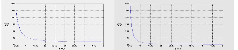
monotone decreasing, which is plotted in Figure2. We havep(0.75)<p(t), q(0.75)>q(t).Hence, Eq.(7) implies t>0.75, while Eq.(8) implies t<0.75. There is a contradiction. Therefore, Z cannot be a GG random variable.It is clear that if Z is GG, the equations (7) and (8) must have the same solution. Solving equations (7) and (8) We can get the solutions t≈0.8033 and t≈0.6260 respectively, which
indicates that Z is not a GG random variable. When the shape parametertakes other values, we can
[image:4.595.96.504.481.567.2]also prove the conclusion with the method employed in the proof in Lemma 4.
Figure 2. Curves forp( ) andq( ) .
The conclusion to the model Z=X+cY is extended, where X, Y are i.i.d with zero means. Since the distribution of Z has nothing with the sign of c as mentioned in Lemma 3, we only consider the case that 0<c≤1.When c=1, the model turns to Z=X+Y. Assuming Z to be a GG random variable with shape parameter t, we can get two equations in the same way employed in the proof Lemma 4.
2 2 2 2 3 3 3 3 ( ) ( ) 1(1 ) ( ) 1 (1 )
t t
c t c
(9)
2 2 4
2 2
(5 ) (1 ) (5 ) (1 )
(1 ) 3 (1 ) 3
(3 ) (3 )
t t c c t
(10)
In order to show the relationship betweenand t, we define thetcurves satisfying equations (9) and (10),which are presented in Figure. 3 for several values of c. In each figure, the curves
Figure 3. -t curves with model Z=X+cY, (a) c=0.5 (b) c=1.
From Figure.3, it is easy to see that if 2, it can’t satisfy equations (9) and (10) at the same time, so Z is no longer GGD. In the other words, Z is a GG random variable if X and Y are Gaussian random variables, and here Z is also a Gaussian random variable. To sum up, the distribution of Z is a kind of new distribution similar to GGD.
Simulation
From the model analysis above, we notice that the distribution of Z is different from GGD, though
there are many similarities between Z and GGD. If we fit Z with GGD modelZGbased on HOS. In this
Section, we will show the relation between Z andZGwith simulation.
Let f z( )andg z( )be the density functions of Z=X+Y and ZG,where X,Y are i.i.d with shape
parameterandZGwith shape parameter t satisfies
2 2 4 4
0, ( ) , ( )
G G G
Z Z Z
E EZ E EZ E EZ (11)
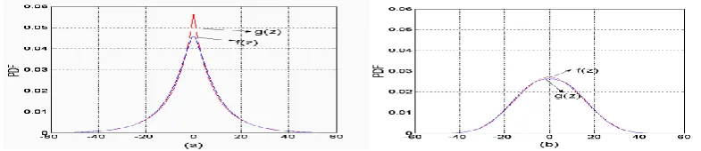
Then t andsatisfy Eq.(6), from which we can get the solution of t. The corresponding shape parameters ofZGare shown in table 1 for=0 and= 0.7, 1, 2 and 3, which are corresponding to the cases that X are super-Gaussian, Gaussian and sub-Gaussian distributions respectively. f z( )andg z( )
are illustrated in Figure.4.
Table 1. The values of t,f(0)andg(0)corresponding to different.
0.7 1 2 3
t 0.8996 1.2568 2 2.3663
f(0) 0.0459 0.0354 0.0282 0.0272 g(0) 0.0576 0.0390 0.0282 0.0262
Table 1shows that if X has super-Gaussian distribution such as=0.7 and 1, so doesZG. Similarly,
if X is Gaussian or sub-Gaussian distribution, it is the same withZG.
Figure 4. The densities of Z and
1
X for several values of, (a)=0.7 (b) =3.
Note that in Figure 4, the two densities coincide with each other well except for the vicinity of zero which is the mean of Z andZG. In addition, g(0)> f(0)whenZGis super- Gaussian distribution in
(a);g(0)< f(0)whenZGis sub- Gaussian in (b).
[image:5.595.96.489.581.666.2]vicinity of zero among the histogram and g(x) as shown in Figure 5. All of these implies that the distribution of Z=X+Y cannot be GGD except that X has Gaussian distribution.
Figue 5. Fitting of histogram with GG density g(z) for several values of (a)=0.7 (b) =3.
Conclusion
The properties of Z=X+Y and GGD were derived. From these properties, we obtained the conclusion that the distribution of the sum of independent GG signals cannot be GGD. As special cases, the PDF
of Z for GG signals with=1 and the proof for GG signals with=½ were given. The simulation
results also lend support to the proposed conclusion and show that there is some difference especially in the vicinity of mean among the densities if applying GGD to model the sum of independent GG signals based on HOS. These properties and results can be useful in analyzing the sum of independent signals with GGD, and the linear system driven by of generalized Gaussian signals.
Acknowledgments
The research was supported by the Nature Science Foundations of Hubei Province (No. 2017CFB730) and the innovative personnel Foundation of Hubei Polytechnic University (No. 14xjz02C) and Major teaching project of Hubei Polytechnic University (No. 2015A08).
References
[1] M L Honig, K Steiglitz, V Balakrishnan, et al. Discrete-time signal design for maximizing separation in amplitude[J]. IEEE Transactions on Information Theory, 2016, 41(1):164-170.
[2] T, Elguebaly, N Bouguila. Bayesian Learning of Generalized Gaussian Mixture Models on Biomedical Images[C]// Iapr Tc3 Conference on Artificial Neural Networks in Pattern Recognition. Springer-Verlag, 2010:207-218.
[3] A. Tesei, and C. S. Regazzoni, "Application to Locally Optimum Detection of Detection of A
New Noise Model", Proc. IEEE ICASSP’96, Vol. 5, pp. 2467-2470, 1996.
[4] J Meuller, X Hu, C Bunthof, et al. Determining intra prediction Mode of Image Coding Unit and Image Decoding Unit[J]. Biochimica Et Biophysica Acta, 2017, 1273(3):191-194.
[5] P Slusarczyk, R Baran. Piecewise-linear subband coding scheme for fast image decomposition[J]. Multimedia Tools & Applications, 2016, 75(17):649-666.
[6] S R Dubey, S K Singh, R K Singh. Multichannel Decoded Local Binary Patterns for Content-Based Image Retrieval[J]. IEEE Transactions on Image Processing A Publication of the IEEE Signal Processing Society, 2016, 25(9):4018-4026.
[7] E Bahar. Computations of the transmission and reflection scattering coefficients in an irregular spheroidal model of the earth-ionosphere waveguide[J]. Radio Science, 2016, 15(5):987-1000.
[9] S S Jin, J Kim, J Park. An investigation of subband decomposition and feature-dimension reduction for musical genre classification [J]. 2017, 36(2):144-150.