R E S E A R C H
Open Access
A selected method for the optimal
parameters of the AOR iteration
Luna Ren
1, Fujiao Ren
1*and Ruiping Wen
2*Correspondence: [email protected] 1Department of Mathematics, Taiyuan Normal University, Taiyuan 030012, Shanxi, P.R. China Full list of author information is available at the end of the article
Abstract
In this paper, we present an optimization technique to find the optimal parameters of the AOR iteration, which just needs to minimize the 2-norm of the residual vector and avoids solving the spectral radius of the iteration matrix of the SOR method.
Meanwhile, numerical results are provided to indicate that the new method is more robust than the AOR method for larger intervals of the parameters
ω
andγ
.Keywords: linear systems; AOR iteration; optimal parameter; optimization
1 Introduction
In recent years, the iterative solvers of a large sparse linear system of equations
Ax=b (.)
are considered in many scientific computing and engineering problems, where the coef-ficient matrixA∈Rn×nis a nonsingular matrix,b∈Rnis a given right-hand vector, and x∈Rnis an unknown vector.
The accelerated overrelaxation (AOR) method, which have been proven to be a pow-erful tool for solving the linear system of equations (.), was introduced firstly by Had-jidimos []. In particular, he showed that when the two parameters are easily obtainable, the AOR method converges faster than the other methods of the same type. Thus, the matter about the determination of the optimal acceleration and overrelaxation parame-ters has to be further investigated. Lots of significant results about the optimal parameparame-ters of the AOR method were given by Hadjidimos []. Analytic formulas about the optimal parameters were put forward by Martins [] in the cases where the coefficient matrixAis a weakly diagonally dominant matrix or anH-matrix. Besides, analytic formulas for optimal parameters were also provided by Hadjidimos [, ] in those cases where the coefficient matrixAis a consistently ordered -cyclic matrix, an irreducibly weakly diagonally domi-nant matrix, anL-matrix, or a real symmetric positive definite matrix. In order to compute the optimal parameters, the spectral radius of the corresponding SOR iteration matrix is required, which may greatly decrease the computing efficiently of the AOR iteration. In addition, the computation of this spectral radius is usually a difficult task. Furthermore, the choice of an analytic formula for a general nonsymmetric matrix is little known to us. Thus, applications of the AOR method to widespread real problems are seriously re-stricted.
The asymptotically optimal successive overrelaxation method of choosing the optimal factor in a dynamic fashion according to known information at the current iterate step was proposed by Bai and Chi []. Besides, a quasi-Chebyshev accelerated iteration method for solving a linear system was presented by Wen, Meng, and Wang [], who obtained the optimal parameter by an optimization model. Similarly, a method of determining the optimal parameter of the SOR method was also introduced by Meng []. Based on the facts mentioned, an optimization technique relating to choosing the optimal parameters is put forward. Here, the optimal parametersωandγ are computed by solving a lower-order nonlinear system that is determined by the residual vector and the coefficient matrixA. Furthermore, the optimal parameters are selected by the Newton iteration method instead of specific analytic formulas in [, , ]. In this study, applying this optimization technique to the AOR iteration, we present a modified method called the asymptotically optimal AOR (AOAOR) method, which is more stable and effective for large linear systems than the AOR method.
In Section , we first briefly review the AOR method and its properties. Then we put forward the AOAOR method in Section . In Section , we use numerical experiments to show the stability of the AOAOR method. We end the paper with conclusions in Section .
2 AOR method and its properties
Hadjidimos [] proposed the following splitting method with two parameters of the coef-ficient matrixA:
A=Mγ,ω–Nγ,ω
with
Mγ,ω=
ω(AD–γAL), Nγ,ω=
ω
( –ω)AD+ (ω–γ)AL+ωAU, (.)
where γ,ω= , AD is the diagonal part ofA, and –AL and –AU are strictly lower and strictly upper triangular parts ofA, respectively. The iteration format of the AOR method for solving the linear systems (.) is
xp+=Lγ,ωxp+gγ,ω,
where
Lγ,ω= (AD–γAL)–
( –ω)AD+ (ω–γ)AL+ωAU, gγ,ω=ω(AD–γAL)–b.
We observe the specific values of the parametersγ andωin [] when the AOR method can be reduced into:
• the Jacobi method ifω= ,γ = ;
• the Simultaneous Overrelaxtion method ifγ = ; • the Gauss-Seidel method ifω= ,γ = ;
• the Successive Overrelaxation method ifω=γ.
Theorem . (Theorems ., ., ., and . of []) Let A be a nonsingular matrix with nonzero diagonal entries.Then {xp}∞
p=generated by the AOR method converges to the unique solution x∗of the linear system(.)in the following cases:
(a) ifAis an irreducibly weakly diagonally dominant matrix;for <γ ≤,a sufficient condition is <ω< γ/[ +ρ(Lγ,γ)];
(b) ifAis a real symmetric positive definite matrix;for <γ < ,a sufficient condition is
<ω< γ/[ +ρ(Lγ,γ)];
(c) ifAis anL-matrix;for <γ ≤,sufficient conditions are
(i) <ω< γ/[ +ρ(Lγ,γ)], (ii)Ais anM-matrix;
(d) ifAis anM-matrix;for≤γ ≤,a sufficient condition is <ω≤max{,+ρ(Lγγ
,γ)}.
Remark In order to compute the optimal parameters, theρ(Lγ,ω) is quite expensive and
may greatly decrease the computing efficiency of the AOR iteration method from Theo-rem .. Hence, the formulas for the optimal parameters in TheoTheo-rem . are only of the-oretical meaning and far away from practical applications. To further derive a reasonably applicable rule for choosing the optimal parameters, the properties of the errors or resid-uals of the AOR method need to be still investigated.
Letεpandrpdenote the error and residual vectors of the AOR method at thepth iterate
step, respectively, that is,εp=xp–x
∗,rp=b–Axp, and let
Hγ,ω=AM–γ,ω–I, (.)
whereM–
γ,ωhas been defined by (.). Then we have the following results.
Theorem . For the AOR method,
(a) ifAis a symmetric positive definite matrix,then:
εp+A=rpTHTγ,ωA–Hγ,ωrp,
∂ ∂γε
p+ A=
ω
rpTHTγ,ωMγ–,ωALM–γ,ωrp,
∂ ∂ωε
p+ A=
ω
rpTHTγ,ωM–γ,ωrp;
(b) ifAis a general nonsymmetric matrix,then:
rp+=rpTHγT,ωHγ,ωrp,
∂ ∂γr
p+ =
ω
rpTHTγ,ωAMγ–,ωALM–γ,ωrp,
∂ ∂ωr
p+ =
ω
rpTHT
γ,ωAM
–
γ,ωrp.
Proof By computing we have
εp+A=εp+,Aεp+=εp+M–
γ,ωrp,Aεp+AM–γ,ωrp
=A––rp+AM–γ,ωrp
, –rp+AM–γ,ωrp
=A–Hγ,ωrp,Hγ,ωrp
=rpTHTγ,ωA–Hγ,ωrp
and
rp+=rp–AM–γ,ωrp,rp–AM–γ,ωrp
=–Hγ,ωrp, –Hγ,ωrp
=rpTHTγ,ωHγ,ωrp.
Because of the equalities
∂(M–
γ,ω)
∂γ = –M –
γ,ω
∂(Mγ,ω)
∂γ M
–
γ,ω and
∂(Mγ,ω)
∂γ = –
ωAL,
∂(M–
γ,ω)
∂ω = –M –
γ,ω
∂(Mγ,ω)
∂ω M
–
γ,ω and
∂(Mγ,ω)
∂ω = –
ω(AD–γAL),
we have
∂(M–
γ,ω)
∂γ =
ωM –
γ,ωALM–γ,ω and
∂(Hγ,ω)
∂γ =
ωAM –
γ,ωALM–γ,ω,
∂(M–
γ,ω)
∂ω =
ωM –
γ,ω and
∂(Hγ,ω)
∂ω =
ωAM –
γ,ω.
Thus,
∂ ∂ωε
p+ A=
rpT
∂H
γ,ω
∂ω T
A–Hγ,ωrp+
rpTHTγ,ωA–
∂Hγ,ω
∂ω r p
=
ω
rpTM–γT,ωHγ,ωrp+
rpTHTγ,ωM–γ,ωrp
=
ω
rpTHTγ,ωM–γ,ωrp,
∂ ∂γε
p+ A=
rpT
∂Hγ,ω
∂γ T
A–Hγ,ωrp+
rpTHTγ,ωA–∂Hγ,ω ∂γ r
p
=
ω
rpTM–γT,ωATLM–γT,ωHγ,ωrp+
rpTHTγ,ωM–γ,ωALM–γ,ωrp
=
ω
rpTHγT,ωMγ–,ωALM–γ,ωrp,
∂ ∂ωr
p+ =
rpT
∂Hγ,ω
∂ω T
Hγ,ωrp+
rpTHγT,ω
∂Hγ,ω
∂ω r p
=
ω
rpTM–γT,ωATHγ,ωrp+
rpTHTγ,ωAM–γ,ωrp
=
ω
∂ ∂γr
p+ =
rpT
∂Hγ,ω
∂γ T
Hγ,ωrp+
rpTHTγ,ω
∂Hγ,ω
∂γ r p
=
ω
rpTM–γT,ωATLMγ–T,ωATHγ,ωrp+
rpTHγT,ωAMγ–,ωALM–γ,ωrp
=
ω
rpTHTγ,ωAMγ–,ωALM–γ,ωrp.
The theorem is proved.
The asymptotically optimal AOR (AOAOR) method for both cases of symmetric posi-tive definite and general nonsymmetric linear systems can be established by Theorem ..
3 The asymptotically optimal AOR method
In this section, we establish the asymptotically optimal AOR method by using the idea of [–].
Since (AD–γAL)–= (I–γL)–A–
D withL=A–DALis a strictly lower triangular matrix, Ln=O(the zero matrix), andρ(γL) < , (I–γL)–can be written in the form of Taylor
expansion ([]). Then
(I–γL)–= n–
k=
(γL)k. (.)
Therefore,M–γ,ωcan be expressed as
M–
γ,ω=ω(AD–γAL)–=ω(I–γL)–A–D =ω n–
k=
(γL)kA–D. (.)
Evidently,M–
γ,ωcan be approximated by a lower-order truncation of the matrix series on
the right-hand side of (.). In general,
M–
γ,ω≈ω
I+αγL+βγLA–D ≡μ(γ,ω,α,β), (.)
whereαandβare two real parameters. In terms of (.) and (.), we have
Hγ,ω=AM–γ,ω–I=ωA
I+αγL+βγLAD––I≡ν(γ,ω,α,β). (.)
Now, applying (.) and (.) to Theorem ., we get the following results:
(a) whenAis a symmetric positive definite matrix,
∂ ∂γε
p+ A≈
ω
rpTν(γ,ω,α,β)Tμ(γ,ω,α,β)ALμ(γ,ω,α,β)rp
= –ωrpTLAD–rp– ωγ αrpTLA–Drp+ωrpTA–DALA–Drp
+ωγαrpTA–DALA–Drp+αrpTAD–LTALA–Drp
+ ωγαβrpTAD–LTALA–Drp
= –ηω– αηωγ+ηω+ (αη+αη)ωγ
+α+βηωγ+ αβηωγ
,
∂ ∂ωε
p+ A≈
ω
rpTν(γ,ω,α,β)Tμ(γ,ω,α,β)rp
= –rpTAD–rp+ωrpTA–DAA–Drp–γ αrpTLA–Drp
–γβrpTLA–Drp+ ωγ αrpTA–DALA–Drp
+ωγβrpTA–DALA–Drp+αrpTA–DLTALA–Drp
+ ωγαβrpTA– D
LTALA– Drp
+ωγβrpTA–DLTALA–Drp
= –η+ηω–αηγ –βηγ+ αηωγ +
βη+αη
ωγ
+ αβηωγ+βηωγ , where ⎧ ⎪ ⎪ ⎪ ⎪ ⎪ ⎪ ⎪ ⎪ ⎪ ⎪ ⎪ ⎪ ⎪ ⎪ ⎪ ⎨ ⎪ ⎪ ⎪ ⎪ ⎪ ⎪ ⎪ ⎪ ⎪ ⎪ ⎪ ⎪ ⎪ ⎪ ⎪ ⎩
η= (rp)TA–Drp, η= (rp)TA–DAA–Drp,
η= (rp)TLA–Drp, η= (rp)TLA–Drp, η= (rp)TA–DALA–Drp, η= (rp)TAD–ALA–Drp,
η= (rp)TAD–LTALA–Drp, η= (rp)TA–D(LT)ALA–Drp, η= (rp)TA–D(LT)ALA–Drp;
(b) whenAis a general nonsymmetric matrix,
∂ ∂γr
p+ ≈
ω
rpTν(γ,ω,α,β)TAμ(γ,ω,α,β)ALμ(γ,ω,α,β)rp
= –ωrpTALA–Drp– ωγ αrpTALA–Drp
+ωrpTA–DATALA–Drp
+ωγαrpTA–DATALA–Drp+αrpTA–DLTATALA–Drp
+ωγα+βrpTA–DLTATALA–Drp
+ ωγαβrpTA– D
LTATALA– Drp
= –ξω– αξωγ +ξω+ (αξ+αξ)ωγ
+α+βξωγ+ αβξωγ
,
∂ ∂ωr
p+ ≈
ω
rpTν(γ,ω,α,β)TAμ(γ,ω,α,β)rp
–γβrpTALA–Drp+ ωγ αrpTA–DATALA–Drp
+ωγβrpTA–DATALA–Drp+αrpTAD–LTATALA–Drp
+ ωγαβrpTA–DLTATALA–Drp
+ωγβrpTA–DLTATALA–Drp
= –ξ+ξω–αξγ –βξγ+αξωγ +
βξ+αξ
ωγ
+ αβξωγ+βξωγ
,
where
⎧ ⎪ ⎪ ⎪ ⎪ ⎪ ⎪ ⎪ ⎪ ⎪ ⎪ ⎪ ⎪ ⎪ ⎪ ⎪ ⎨ ⎪ ⎪ ⎪ ⎪ ⎪ ⎪ ⎪ ⎪ ⎪ ⎪ ⎪ ⎪ ⎪ ⎪ ⎪ ⎩
ξ= (rp)TAA–Drp, ξ= (rp)TAD–ATAA–Drp, ξ= (rp)TALA–Drp,
ξ= (rp)TALA–Drp, ξ= (rp)TAD–ATALA–Drp, ξ= (rp)TA–D(LT)ATAA–Drp, ξ= (rp)TA–DLTATALA–Drp,
ξ= (rp)TA–D(LT)ATALA–Drp, ξ= (rp)TA–D(LT)ATALA–Drp.
Our discussion can be summarized as the following theorems.
Theorem . Let A be a symmetric positive definite matrix.Then reasonable
approxima-tionsγp,ωpsatisfyingarg min>ω≥γ>εp+Aare given by solving the nonlinear system ⎧
⎪ ⎪ ⎪ ⎨ ⎪ ⎪ ⎪ ⎩
–ηˆω– αηˆωγ+ηˆω+ (αηˆ+αηˆ)ωγ + (α+β)ηˆωγ
+ αβηˆωγ= ,
–ηˆ+ηˆω–αηˆγ –βηˆγ+ αηˆωγ+ (βηˆ+αηˆ)ωγ
+ αβηˆωγ+βηˆωγ= ,
(.)
where
ρ=A–Drp, ρ=Lρ, ρ=Aρ,
ρ=Aρ, ρ=Lρ, ρ=Aρ.
(.)
Hence,
⎧ ⎪ ⎨ ⎪ ⎩
ˆ
η= (rp)Tρ, ηˆ=ρTρ, ηˆ= (rp)Tρ,
ˆ
η= (rp)Tρ, ηˆ=ρTρ, ηˆ=ρTρ,
ˆ
η=ρTρ, ηˆ=ρTρ, ηˆ=ρTρ.
Theorem . Let A be a general nonsymmetric matrix.Then reasonable approximations γp,ωpsatisfyingarg min
>ω≥γ>rp+are given by solving the nonlinear system ⎧
⎪ ⎪ ⎪ ⎨ ⎪ ⎪ ⎪ ⎩
–ξˆω– αξˆωγ +ξˆω+ (αξˆ+αξˆ)ωγ + (α+β)ξˆωγ
+ αβξˆωγ= ,
–ˆξ+ξˆω–αξˆγ –βξˆγ+ αξˆωγ+ (βξˆ+αξˆ)ωγ
+ αβξˆωγ+βξˆωγ= ,
(.)
where
δ=A–Drp, δ=Aδ, δ=Lδ,
δ=Aδ, δ=Lδ, δ=Aδ.
(.)
Hence,
⎧ ⎪ ⎨ ⎪ ⎩
ˆ
ξ= (rp)Tδ, ξˆ=δTδ, ξˆ= (rp)Tδ,
ˆ
ξ= (rp)Tδ, ξˆ=δTδ, ξˆ=δTδ,
ˆ
ξ=δTδ, ξˆ=δTδ, ξˆ=δTδ.
(.)
By Theorems .-. the asymptotically optimal AOR (AOAOR) method can be con-structed for the cases whereAis a symmetric positive definite matrix or a general non-symmetric matrix.
Method .(AOAOR method for a symmetric positive definite matrix)
S. Given an initial vectorx∈Rn, a precisionε
, and two parametersα,β, for p= , , , . . .:
S. Computerp=b–Axp.
S. Compute (.). S. Compute (.).
S. Solve (.) by the Newton method (see []) for obtainingγp,ωp. S. Determineγp,ωpthat make the Hessian matrix positive definite.
S. Solve(AD–γAL)yp=rpto getyp.
S. Computexp+=xp+ωyp.
Method .(AOAOR method for a nonsymmetric matrix)
S. Given an initial vectorx∈Rn, a precisionε
, and two parametersα,β, for p= , , , . . .:
S. Computerp=b–Axp. S. Compute (.). S. Compute (.).
S. Solve (.) by the Newton method (see []) for obtainingγp,ωp.
S. Determineγp,ωpthat make the Hessian matrix positive definite. S. Solve(AD–γAL)yp=rpto getyp.
S. Computexp+=xp+ωyp.
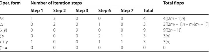
Methods .-. both shared the same cost. Method . requires nine vectorsx,y,r,ρi
Table 1 Operation forms and flops at each step of the iteration
Oper. form Number of iteration steps Total flops
Step 1 Step 2 Step 3 Step 6 Step 7 Total
Ax 1 3 0 0 0 4 4[(2m– 1)n]
Lx 0 2 0 1 0 3 3[(2ml– 1)n–ml(ml– 1)]
(x,y) 0 0 9 0 0 9 9[(2n– 1)]
ζy 0 0 0 2 1 3 3[n]
x+y 1 0 0 1 1 3 3[n]
ζ·κ 0 0 0 0 0 0 0
nine inner products (S of Method .), three operations of the formζx, three operations of the formx+y, and no operations of the formζ κ, whereζ andκare scalars. Thus, if the number of nonzero entries on each row of the matrixAismand that of the matrixLis
ml, then the details are listed in Table .
4 Numerical experiments
The test example is the following two-dimensional partial differential equation with Dirichlet boundary condition ([]):
–∂∂u
t –
∂u
∂t +
ξ∂∂tu
+ζ
∂u
∂t+ σu=f(t,t), (t,t)∈,
u(t,t) = , (t,t)∈∂,
(.)
whereξ, ζ, andσ are all constants, is the unit square (, )×(, ) inR,∂is the
boundary of the domain, andf(t,t) :→Ris a given function.
Ifui,jandfi,jdenote the approximate solution of (.) and an approximation of the
func-tionf(t,t) at the grid point (ih,jh), respectively, then a discretized approximation of (.)
is the following linear system of equations:
μui+,j+ηui–,j+μui,j++ηui,j–+μui,j=hfi,j, i,j= , , . . . ,N, (.)
where (N+ )h= , and
μ= ( +σh), μ= –( –ξh), μ= –( –ζh),
η= –( +ξh), η= –( +ζh).
Let
xT= (u,, . . . ,u,N,u,, . . . ,u,N, . . . ,uN,, . . . ,uN,N).
The linear system (.) can be written as the linear system (.) with
A=
⎛ ⎜ ⎜ ⎜ ⎜ ⎜ ⎜ ⎜ ⎝
T μI ηI T μI
. .. . .. ...
ηI T μI ηI T
⎞ ⎟ ⎟ ⎟ ⎟ ⎟ ⎟ ⎟ ⎠
with
T=
⎛ ⎜ ⎜ ⎜ ⎜ ⎜ ⎜ ⎜ ⎝
μ μ η μ μ
. .. ... ...
η μ μ η μ
⎞ ⎟ ⎟ ⎟ ⎟ ⎟ ⎟ ⎟ ⎠
∈RN×N
and
bT=h(f,, . . . ,f,N,f,, . . . ,f,N, . . . ,fN,, . . . ,fN,N),
wheren=N×N.
In practical computations, the right-hand sideb is generated byb=Ae, in whiche= (, , . . . , )T∈Rn, the initial vectorx∈Rnis taken to be zero, and all runs are terminated
if the current iteration satisfies either the value of residual
RES≡rp ≤εr
(.)
or the number of iteration steps exceeds ,. The iteration indexp, namely, the number of iteration steps satisfying (.), is particularly denoted as “IT”, and the running time in seconds is denoted as “CPU”. In addition, all experiments are performed in MATLAB Ra on PC with . GHz processor, GB memory, and -bit operating system, “†” indicates that the number of iterations is greater than ,, that is, the iteration fails, “-” indicates that the computing is out of memory.
With different selections ofξ,ζ,σ, different forms of the coefficient matrix are given. Particularly, the coefficient matrixAis a symmetric matrix whenξ =ζ =σ= . orξ=
ζ = .,σ= ., and it is a nonsymmetric matrix forξ= .,ζ= .,σ= . orξ= .,
ζ = .,σ= .. In Tables -, we list the numbers of iteration steps, the -norms of the residual vectors, and the computing times for different choices ofξ,ζ,σ.
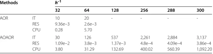
From Tables - we can see that although the IT and CPU of the AOR method are less than those of the AOAOR method whenh–< , the AOR method is out of memory,
whereas the AOAOR method can continue to run forh–≥. Moreover, in the iteration process, (AD–γAL)–of dimensionNrequires to be solved for the AOR method. The AOAOR method, however, only needs to solve the inverse ofN-dimensionalT. Thus, the AOAOR method is better than the AOR method with respect to the increase of the size of the coefficient matrix.
Table 2 Numerical results whenξ=ζ=σ= 0.0 (ε=h2/5)
Methods h–1
32 64 128 256 288 300
AOR IT 41 89 - - -
-RES 1.9e–3 7.38e–4
CPU 0.20 4.18
AOAOR IT 216 895 3,816 16,200 † †
RES 2.1e–3 7.68e–4 2.76e–4 9.71e–5
[image:11.595.118.479.234.324.2]CPU 10.84 58.96 275.80 2,300.30
Table 3 Numerical results whenξ=ζ= 0,σ= 2.5 (ε=h2/5)
Methods h–1
32 64 128 256 288 300
AOR IT 36 78 - - -
-RES 1.86e–3 7.0e–4
CPU 0.18 4.08
AOAOR IT 154 641 2,688 11,613 † †
RES 2.1e–3 7.8e–4 2.7e–4 9.75e–5
CPU 7.74 40.31 189.08 1,560.23
Table 4 Numerical results whenξ= 30.0,ζ= 0.0,σ= 10.0 (ε=h2)
Methods h–1
32 64 128 256 288 300
AOR IT 23 51 - - -
-RES 9.99e–3 3.42e–3
CPU 0.18 3.64
AOAOR IT 61 259 1,078 4,526 5,772 6,279
RES 1.18e–2 3.9e–3 1.38e–3 4.8e–4 4.1e–3 3.86e–4
CPU 2.54 13.21 52.06 288.58 379.42 434.97
Table 5 Numerical results whenξ= 0.0,ζ= 30.0,σ= 10.0 (ε=h2)
Methods h–1
32 64 128 256 288 300
AOR IT 10 20 - - -
-RES 9.36e–3 2.6e–3
CPU 0.28 5.70
AOAOR IT 30 126 537 2,261 2,884 3,137
RES 1.09e–2 3.8e–3 1.37e–3 4.8e–4 4.09e–4 3.86e–4
CPU 3.80 31.29 132.69 400.02 560.39 1,092.20
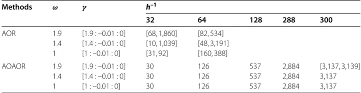
From Tables - we note that:
(a) Whenωis a specific value, as forω= .andh–= , the IT of the AOR method is
[image:11.595.118.479.368.460.2] [image:11.595.118.479.503.595.2]Table 6 The gap of IT whenξ=ζ=σ= 0.0 (ε=h2/5)
Methods ω γ h–1
32 64 128 256
AOR 1.9 [1.9 : –0.01 : 0] [95, 782] [120, 2,822] 1.4 [1.4 : –0.01 : 0] [121, 1,699] [513, 8,265] 1 [1 : –0.01 : 0] [282, 573] [1,197, 2,438]
AOAOR 1.9 [1.9 : –0.01 : 0] 216 [895, 916] [3,904, 3,907] 16,200
1.4 [1.4 : –0.01 : 0] 216 [896, 903] 3,907 16,200
[image:12.595.118.480.235.328.2]1 [1 : –0.01 : 0] 216 [896, 906] [3,901, 3,907] 16,200
Table 7 The gap of IT whenξ=ζ= 0.0,σ= 2.5 (ε=h2/5)
Methods ω γ h–1
32 64 128 256
AOR 1.9 [1.9 : –0.01 : 0] [95, 529] [120, 4,585] 1.4 [1.4 : –0.01 : 0] [87, 7,872] [365, 1,305] 1 [1 : –0.01 : 0] [202, 405] [852, 1,715]
AOAOR 1.9 [1.9 : –0.01 : 0] 154 641 [2,689, 2,709] 11,613
1.4 [1.4 : –0.01 : 0] 154 641 [2,693, 2,701] 11,613
1 [1 : –0.01 : 0] 154 641 [2,688, 2,703] 11,613
Table 8 The gap of IT whenξ= 30.0,ζ= 0.0,σ= 10.0 (ε=h2)
Methods ω γ h–1
32 64 128 288 300
AOR 1.9 [1.9 : –0.01 : 0] [199, 1,824] [215, 526] 1.4 [1.4 : –0.01 : 0] [23, 2,765] [84, 1,137] 1 [1 : –0.01 : 0] [50, 96] [196, 387]
AOAOR 1.9 [1.9 : –0.01 : 0] 61 259 [1,078, 1,081] 5,772 6,279 1.4 [1.4 : –0.01 : 0] 61 259 [1,079, 1,081] 5,772 6,279 1 [1 : –0.01 : 0] 61 259 [1,079, 1,081] 5,772 6,279
Table 9 The gap of IT whenξ= 0.0,ζ= 30.0,σ= 10.0 (ε=h2)
Methods ω γ h–1
32 64 128 288 300
AOR 1.9 [1.9 : –0.01 : 0] [68, 1,860] [82, 534] 1.4 [1.4 : –0.01 : 0] [10, 1,039] [48, 3,191] 1 [1 : –0.01 : 0] [31, 92] [160, 388]
AOAOR 1.9 [1.9 : –0.01 : 0] 30 126 537 2,884 [3,137, 3,139]
1.4 [1.4 : –0.01 : 0] 30 126 537 2,884 3,137
1 [1 : –0.01 : 0] 30 126 537 2,884 3,137
(b) Whenωis variable andγ is a suitable fixed value, the minimal IT of the AOR method is forω= .andh–= , and it is forω= andh–= in Table .
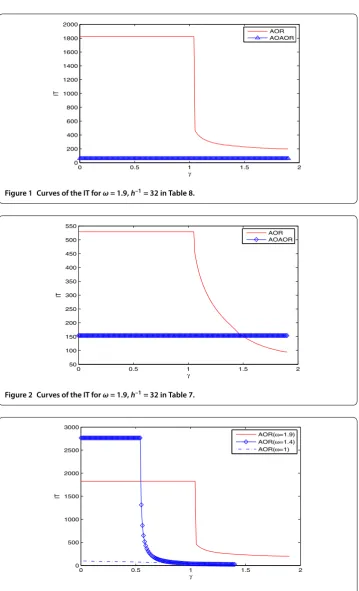
[image:12.595.116.479.373.466.2] [image:12.595.116.478.509.602.2]Figure 1 Curves of the IT forω= 1.9,h–1= 32 in Table 8.
Figure 2 Curves of the IT forω= 1.9,h–1= 32 in Table 7.
Figure 3 Curves of the IT forω= 1.9,ω= 1.4, andω= 1 withh–1= 32 in Table 8.
Figure clearly depicts the variation with respect toω. We notice that the graph of the AOR method is vertically descending, whereas that of the AOAOR method is completely flat, which shows that the IT of the AOAOR method is independent of the choice ofγ. So does Figure .
Whenωis not an exact value, the numbers of IT of the AOR method are dramatically different for invariableγ, that is, it depends on the choice ofω. However, the IT of the AOAOR method remains at . Therefore, the conclusion that the IT of the AOAOR method is independent of the choice ofωis illustrated in Figure .
Thus, from Figures - we see that both AOR and AOAOR methods are sensitive to the parametersωandγ. For the larger intervals of the parametersωandγ, the IT of the AOR method varies according to the curve wave; however, that of the AOAOR method is almost at the same level. This means that the AOR method is more sensitive to the initial guesses of the optimal parametersωandγ, whereas the AOAOR method is more stable.
5 Conclusions
The asymptotically optimal accelerated overrelaxation (AOAOR) method for linear sys-tems (.) has been presented. Especially, the optimal parameters are discussed. The nu-merical experiments have shown that the AOAOR method is efficient when the dimension of the coefficient matrix is over . Furthermore, the AOAOR method is more stable with
respect the initial guesses of relaxation factorsωandγ.
Competing interests
The authors declare that they have no competing interests.
Authors’ contributions
All authors contributed equally to the writing of this paper. All authors read and approved the final manuscript.
Author details
1Department of Mathematics, Taiyuan Normal University, Taiyuan 030012, Shanxi, P.R. China.2Higher Education Key Laboratory of Engineering and Scientific Computing, Taiyuan Normal University, Taiyuan 030012, Shanxi, P.R. China.
Acknowledgements
The authors are very much indebted to the anonymous referees for their helpful comments and suggestions, which greatly improved the original manuscript of this paper. This work is supported by grants from the NSF of Shanxi Province (201601D011004).
Received: 30 June 2016 Accepted: 4 October 2016
References
1. Hadiiidmos, A: Accelerated overrelaxation method. Math. Comput.32, 149-157 (1978)
2. Hadiiidmos, A: A survey of the iterative methods for the solution of linear systems by extrapolation, relaxation and other techniques. J. Comput. Appl. Math.20, 37-51 (1987)
3. Martins, MM: Generalized diagonal dominance in connection with the accelerated overrelaxation method. BIT Numer. Math.22, 73-78 (1982)
4. Hadiiidmos, A, Yeyios, A: The principle of extrapolation in connection with the accelerated overrelaxation method. Linear Algebra Appl.30, 115-128 (1980)
5. Bai, ZZ Chi, XB: Asymptotically optimal successive overrelaxation method for systems of linear equations. J. Comput. Math.21(5), 503-612 (2003)
6. Wen, RP, Meng, GY, Wang, CL: Quasi-Chebyshev accelerated iteration methods based on optimization for linear systems. Comput. Math. Appl.66, 934-942 (2013)
7. Meng, GY: A practical asymptotical optimal SOR method. Appl. Math. Comput.242, 707-715 (2014)
8. Hadiiidmos, A, Yeyios, A: On some extensions of the accelerated overrelaxation (AOR) theory. J. Math. Sci.5, 49-60 (1982)
9. Higham, NJ: Functions of Matrices Theory and Computation. SIAM, Philadelphia (2008)