R E S E A R C H
Open Access
A Schrödinger-type algorithm for solving the
Schrödinger equations via
Phragmén–Lindelöf inequalities
Lingling Zhao
1**Correspondence:
[email protected] 1School of Information and Electrical Engineering, Ludong University, Yantai, P.R. China
Abstract
In this article, we consider the numerical method for solving the Schrödinger equations via Phragmén–Lindelöf inequalities under the order induced by a symmetric cone with the function involved being monotone. Based on the
Phragmén–Lindelöf inequalities, the underlying system of inequalities is reformulated as a system of smooth equations, and a Schrödinger-type method is proposed to solve it iteratively so that a solution of the system of the Schrödinger equations is found. By means of the Schrödinger type inequalities, the algorithm is proved to be well defined and to be globally convergent under weak assumptions and locally quadratically convergent under suitable assumptions. Preliminary numerical results indicate that the algorithm is effective.
Keywords: Schrödinger equation; Phragmén–Lindelöf inequality; Schrödinger type inequality; Convergence
1 Introduction
In this paper, we consider the following Schrödinger equation (see [18,19]):
–u+V(x)u=
1
|x|α ∗ |u|
p
|u|p–2u, x∈ n, (1.1)
wheren≥3, 0 <α<n, 2 –α
n<p≤2∗α=2nn–2–α and
(A1) V∈C(Rn,R+)is coercive, that is,
lim
|x|→+∞V(x) = +∞.
In 2016, Qiao et al. [19] first considered the bound and ground states for the nonlinear Schrödinger equations under the condition
(A2) infRnV> 0, and there exists a positive constantrsatisfying
measx∈Rn,|x–y| ≤r,V(x)≤M→0
as|y| → ∞, whereM> 0and meas stands for the Lebesgue measure.
The nonlinear system (1.1) has been proved to possess wide application fields in many real world problems such as anomalous diffusion [2,4,15], disease models [6,9,21], eco-logical models [26], synchronization of chaotic systems [1,27], etc.
Put
ν(x) :=1 2u(x)
2
is the Nevanlinna norm (see [8]), problem (1.1) is equivalent to the following Schrödinger problem defined by
minν(x), (1.2)
wherex∈ n.
The Phragmén–Lindelöf inequalities (see [23]) have the main objective to solve the so-called Schrödinger Phragmén–Lindelöf subproblem model to get the trial stepτk
Min T Wk(τ) =1
2u(xk) +∇S(xk)τ
2
,
τ ≤ .
In 2015, a modified Phragmén–Lindelöf inequality was proved by Wan [23]:
Min φk(τ) =1
2u(xk) +∇u(xk)τ
2
,
τ ≤cpu(xk)γ,
wherep,c, andγ are three positive numbers.
Recently, another adaptive Schrödinger Phragmén–Lindelöf inequality has been defined by Qiao et al. [17]:
Min T Mk(τ) =1
2u(xk) +Bkτ
2
,
τ ≤cpu(xk),
(1.3)
whereBkis defined by
Bk+1=Bk–Bk
sksTk Bk
sTk Bksk +ykyk
T
ykTsk
, (1.4)
We further consider the Schrödinger Phragmén–Lindelöf model for the nonlinear sys-temu(x) atxk(see [17])
ϑ(xk+τ) =u(xk) +∇u(xk)Td+ 1 2Tkd
2, (1.5)
where∇u(xk) is the Jacobian matrix ofu(x) atxk.
It is well known that the above model (1.5) can be written as the following extension (see [20,23,24]):
ϑ(xk+τ) =u(xk) +∇u(xk)Td+ 3 2
sTk–1τ2sk–1. (1.6)
If we set the Schrödinger Phragmén–Lindelöf matrix ∇u(xk), then we can use the Schrödinger Phragmén–Lindelöf matrix Bk instead of it. Thus, our Schrödinger Phragmén–Lindelöf model can be defined as follows:
Min Nk(τ) = 1 2
u(xk) +Bkd+ 3 2
sTk–1τ2sk–1
2,
τ ≤cpu(xk)γ,
(1.7)
whereBk=Hk–1andHkis generated by
Hk+1=VkTHkVk+ρksksTk
=VkT VkT–1Hk–1Vk–1+ρk–1sk–1sTk–1
Vk+ρksksTk =· · ·
= VkT· · ·VkT–m+1Hk–m+1[Vk–m+1· · ·Vk]
+ρk–m+1 VkT–1· · ·VkT–m+2
sk–m+1sTk–m+1[Vk–m+2· · ·Vk–1]
+· · ·
+ρksksTk, (1.8)
whereρk=sT1
k yk,Vk=I–
ρkyksTk (see [23] etc.). Letτkpbe the solution of (1.7). Define
Aτk
τkp=νxk+τkp
–ν(xk), (1.9)
and predict reduction by
Pτk
τkp=Nk
τkp–Nk(0). (1.10)
Based on definitions ofAτk(τkp) andPτk(τkp), we design their ratio by
rpk= Aτk(τ p k)
Pτk(τkp). (1.11)
Algorithm
Initial: LetB0=H–10 ∈ n×nbe a symmetric and positive definite matrix.x0∈ nand
= 0.ρ,c, andare three positive constants. Letl:= 0; Step 1: Stop ifχ(xl)<holds;
Step 2: Solve (1.7) with=lto obtainςl;
Step 3: ComputeAςl(ςl),Pςl(ςl), and the ratiorl. Ifrl <ρ, let=+ 1, go to Step 2. Ifrl≥ρ, go to the next step;
Step 4: Set xl+1=xl+ςl,yl=χ(xl+1) –χ(xl), updateBl+1=H–1l+1 by (1.8) ifyTl ς p l > 0,
otherwise setBl+1=Bl;
Step 5: Letl:=l+ 1and= 0. Go to Step 1.
In this paper, we further focus on convergence results of the above algorithm under the following assumptions.
Assumptions
(A) Define the setΩby
Ω=x|ϕ(x)≤ϕ(x0)
. (1.12)
It is easy to see thatΩis bounded.
(B) The nonlinear system χ(x)is twice continuously differentiable inΩ1, which is an
open convex set containingΩ.
(C) The following Phragmén–Lindelöf relation
∇χ(xl) –Bl
χ(xl)=Oςlp (1.13)
holds.
(D) The sequence matrices{Bl}are uniformly bounded inΩ1.
It follows from Assumption (B) that (see [10,22])
∇χ(xl)T∇χ
(xl)≤ML, (1.14)
whereMLis a positive real number.
2 Convergence results
We first have the following new Phragmén–Lindelöf inequalities.
Lemma 2.1 Letτkpbe the solution of(1.1).Then
Pτk
τkp≤–1
2Bku(xk)min
k,Bku(xk)
Ml2
+O2k (2.1)
holds.
Proof Define
J(u) =1 2
n|∇
u|2+u2dx– 1 2p
n
n
|u(x)|p|u(y)|p
It follows from (1.7) that
j0<j1=inf
N–J(u) <j0+
p– 1 2p S
p p–1 α,p.
ConsiderV(x) is a minimizer for bothSα,p. By the continuity ofJ, we know that
J(u0+tV) <j0+
p– 1 2p S
p p–1 α,p,
where 0≤t<γ. So
J(u0+tV) =
1
2u0+tV
2– 1
2pB˜(u0+tV) –
nh(u0+tV)dx
=J(u0) +
t2
2
V2–t p–2
p B˜(V)
+B˜(u0) +B˜(tV) –B˜(u0+tV)
<j0+
p– 1 2p S
p p–1 α,p.
It follows fromt≥γ that
J(u0+tV) =
1
2u0+tV
2– 1
2pB˜(u0+tV) –
nh(u0+tV)dx
=1 2u0
2+t
n∇
u0∇V+u0V dx+
t2
2V
2– 1
2pB˜(u0)
+ 1
2p B˜(u0) +B˜(tV) –B˜(u0+tV)
– 1 2pB˜(tV)
–
nhu0dx–
nhtV dx
=J(u0) +
t2
2
V2–t
2(p–1)
2p B˜(V)
+ 1 2p
˜
B(u0) +B˜(tV)
–B˜(u0+tV) + 2p
n
n
|u0(x)|p|u0(y)|p–2u0(y)
|x–y|α dx dy
<j0+
p– 1 2p S
p p–1 α,p.
Here, we use thatJ(u0),tV= 0 andV(x) is a solution of (1.1). By the definition ofτkp [14,16] and it being the solution of (1.7), we get
Pτk
τkp≤Pτk
–α k
Bku(xk)
Bku(xk)
= 1 2
α22kBkBku(xk)
2
Bku(xk)2
+α44k9
4
(sTk–1Bku(xk))4
Bku(xk)4
+ 3α22k(s
T
k–1Bku(xk))2
Bksk–12
u(xk)Tsk–1– 2αk
(u(xk)TBkBku(xk))
Bku(xk)
– 3α33k(s
T
k–1Bku(xk))2sTk–1BkBku(xk)
Bku(xk)3
= 1 2
α22kBkBku(xk)
2
Bku(xk)2
– 2αk
(u(xk)TBkBku(xk))
Bku(xk)
+O2k
≤–αkBku(xk)+ 1 2α
22
kM2l +O
2
k
for anyα∈[0, 1]. Therefore
Pτk
τkp≤ min 0≤α≤1
–αkBku(xk)+ 1 2α
22
kM2l
+O2k
≤–1
2Bku(xk)min
k,Bku(xk)
M2
l
+O2k.
Lemma 2.2 Let Assumptions(A), (B), (C),and(D)hold.Then
Aτk
τkp–Pτk
τkp=Oτkp2,
whereτkis the solution of(1.7).
Proof It follows from (1.9) and (1.10) that
Aτk
τkp–Pτk
τkp=νxk+τkp
–Nk
τkp
= 1 2
u(xk) +∇u(xk)τkp+Oτkp22
–u(xk) +Bkτkp+ 3 2
sTk–1τkp2sk–1
2
=u(xk)T∇u(xk)τkp–u(xk)TBkτkp+Oτ p k
2
+Oτkp3+Oτkp4
≤ ∇u(xk) –Bk
u(xk)τkp+Oτkp2
+Oτkp3+Oτkp4
=Oτkp2.
Theorem 2.1 Let Assumptions(A), (B), (C),and(D)hold.Then Algorithm either finitely stops or generates an infinite sequence{xk}satisfying
lim
k→∞u(xk)= 0, (2.2)
where{xk}is defined as in Algorithm.
Proof We know thatt–(u) is a continuous function ofu. Consequently, the manifoldΛ–
disconnectsD1,2(n) in exactly two connected componentsU1andU2, where
U1=
u∈D1,2n:u= 0 oruD<t–
u uD
,
U2=
u∈D1,2n:uD>t–
u uD
SoD1,2(n) =Λ–∪U
1∪U2. In particular,u0∈Λ+⊂U1. Since
t–
u0+tW
u0+tWD
u0+tW
u0+tWD ∈
Λ,
we have
0 <t–
u0+tW
u0+tWD
<C0
uniformly fort∈R. On the other hand,
u0+tWD≥tWD–u0D≥C0,
wheret≥ ˜t.
So that we can fix a positive numbert0such that
u0+t0WD>t–
u0+t0W
u0+t0WD
,
which yields that
u0+t0W∈U2.
Combining this and the factu0∈U1, we know that
u0+t1W∈Λ–
for some 0 <t1<t0.
So
c1=inf
Λ–I(u)≤0max≤t≤t 0
I(u0+tW) <c0+
N+ 2 –α
4N– 2α S
2N–α N+2–α H,L .
And there exists a minimizing sequence{un} ⊂Λ–satisfying
I(un) <c1+
1
n;
I(w)≥I(un) –1
nu–wD,
wherew∈Λ–. So that
c1+ 1 >I(un) =
1 2un
2
D– 1
2·2∗αB(un) –
nh(x)undx
≥
1 2–
1 2·2∗α
un2D–
1 – 1
2·2∗α
hH–1unD,
It follows from{un} ⊂Λ–that
un2D≤
2·2∗α– 1un
2∗α D
S2∗α H,L
.
Thus,unDhas a uniform positive lower bound. Similarly,
I(un)→c1, I(un)→0 inH–1.
By Lemma2.2and
c1<c0+
N+ 2 –α
4N– 2α S
2N–α N+2–α H,L ,
we obtain that
nh(x)u1dx> 0 and u1∈
Λ+,
which leads to a contradiction.
In the caseh> 0. Applying Lemma2.1tou1and|u1|, we know that there existst–(|u1|)
such that
t–|u1|
|u1| ∈Λ–.
Moreover,
t–|u1|
≥t0
|u1|
=t0(u1) =
A(u1)
(2∗α– 1)B(u1)
1 2∗α–2
.
So
nh(x)u1dx=
nh(x)|u1|dx,
which implies thatu1≥0. According to the maximum principle, we getu1> 0.
It is easy to see thatunis bounded, which yields that
un2=wn2+v2+o(1), n→ ∞,
and
n
|wn(x)|p|wn(y)|p
|x–y|α dw
=
n
|wn(x)|p|wn(y)|p
|x–y|α dw+
n
|w(x)|p|w(y)|p
|x–y|α dw+on(1)
So
c←J(wn) = 1 2wn
2– 1
2p
n
|wn(x)|p|wn(y)|p
|x–y|α dw–
nh(x)wndx
=1 2wn
2– 1
2p
n
|wn(x)|p|wn(y)|p
|x–y|α dw–
nh(x)wndx
+1 2v
2– 1
2p
n
|v(x)|p|v(y)|p
|x–y|α dw–
nh(x)v dx+on(1)
=J(v) +1 2wn
2– 1
2pB˜(wn) +on(1)
and
1 2wn
2– 1
2pB˜(wn) +on(1) < p– 1
2p S
p p–1
α,p. (2.3)
Notice that
o(1) =J(un),un
=J(v),v+wn2–B˜(wn) +o(1),
which yields that
wn2–B˜(wn) =o(1). (2.4)
It follows from (2.4) that
wn2=B˜(wn)≤
wn2p
Spα,p
and
1 2
p– 1
p S
p p–1 α,p =
1 2
1 –1
p
S
p p–1
≤1
2
1 –1
p
wn2
=1 2wn
2– 1
2pB˜(wn) +on(1)
<p– 1 2p S
p p–1 α,p,
which also leads to a contradiction. Suppose that
lim
k→∞Bku(xk)= 0 (2.5)
holds. Using Assumption (C) we get (2.2). It follows from (2.5) that the subsequence{kj} satisfies
Set
K=k|Bku(xk)≥ε
.
So we assume that
u(xk)≥ε
holds, wherek∈K.
It follows from the definition of Algorithm and Lemma2.1that
k∈K
ν(xk) –ν(xk+1)
≥–
k∈K
ρPτk
τpk k
≥
k∈K
ρ1
2min
cpkε, ε
M2l
ε.
Lemma2.2gives us that the sequence{ν(xk)}is convergent, which yields that
k∈K
ρ1
2min
cpkε, ε
M2
l
ε< +∞.
Thenpk→+∞whenk→+∞andk∈K. It follows that
min qk(τ) =1 2
u(xk) +Bkτ+ 3 2
sTk–1τ2sk–1
2,
s.t. τ ≤cpk–1u(xk)
(2.7)
is unacceptable.
If we putxk+1=xk+τk, then we have
ν(xk) –ν(xk+1)
–Pτk(τk)
<ρ. (2.8)
By applying Lemma2.1and the definition ofk, we know that
–Pτk
τk≥1
2min
cpk–1ε, ε
M2
l
ε.
By applying Lemma2.2, we know that
νxk+1–ν(xk) –Pτk
τk=Oτk2=Oc2(pk–1). So
ν(xk+1) –ν(xk)
Pτk(τk) – 1
≤ O(c2(pk–1))
0.5min{cpk–1ε, ε
M2l}ε+O(c
2(pk–1)ε2). By applyingpk→+∞ask→+∞, we know that
ν(xk) –ν(xk+1)
–Pτk(τk) →1, k∈K,
3 Numerical results
This section reports some numerical results of Algorithm.
3.1 Problems
Define
u(x) =υ1(x),υ2(x), . . . ,υn(x)
T
.
Problem 1 The Schrödinger differential function (see [12])
υl(x) = 2
n+l(1 –cosxl) –sinxl– n
j=1 cosxj
(2sinxl–cosxl),
wherel= 1, 2, 3, . . . ,n.
Initial guess:
x0=
101 100n,
101 100n, . . . ,
101 100n
T
.
Problem 2 Logarithmic function
υl(x) =ln(xl+ 1) –
xl
n,
wherel= 1, 2, 3, . . . ,n.
Initial points:
x0= (1, 1, . . . , 1)T.
Problem 3 Schrödinger differential function (see [5, pp. 471–472])
υ1(x) = (2 – 0.2x1)x1–x2+ 1,
υl(x) = (2 – 0.2xl)xl–xi–1+xi+1+ 1,
υn(x) = (2 – 0.2xn)xn–xn–1+ 1,
wherel= 1, 2, 3, . . . ,n.
Initial points:
x0= (–1, –1, . . . , –1)T.
Problem 4 Trigexp function (see [5, p. 473])
υ1(x) = 3x31+x2– 4 + 2sin(x1–x2)sin(x1+x2),
υl(x) = –2xi–1exi–1–xl+ 3xl
–sin(xl–xi+1)sin(xl+xi+1) – 2,
υn(x) = –2xn–1exn–1–xn+ 3xn– 2, wherel= 1, 2, 3, . . . ,n.
Initial guess:
x0= (0, 0, . . . , 0)T.
Problem 5 Letu(x) be the gradient of
h(x) = n
l=1
exl–x
l
.
Then
υl(x) =exl– 1, wherel= 1, 2, 3, . . . ,n.
Initial points:
x0=
1
n,
2
n, . . . , 1 T
.
Parameters:c= 0.2,= 10–2,ρ= 0.03,p= 3,m= 6H
0is the unit matrix.
The method for(1.3)and(1.7): theDoglegmethod [13,25].
Code experiments: run on a PC with Intel Pentium(R) Xeon(R) E5507 CPU 2.27 GHz, 6.00 GB of RAM, and Windows 7 operating system.
Code software: MATLAB r2017a.
Stop rules: the program stops ifu(x) ≤1e– 4 holds.
Other cases: we will stop the program if the iteration number is larger than ten hundred.
3.2 Results and discussion
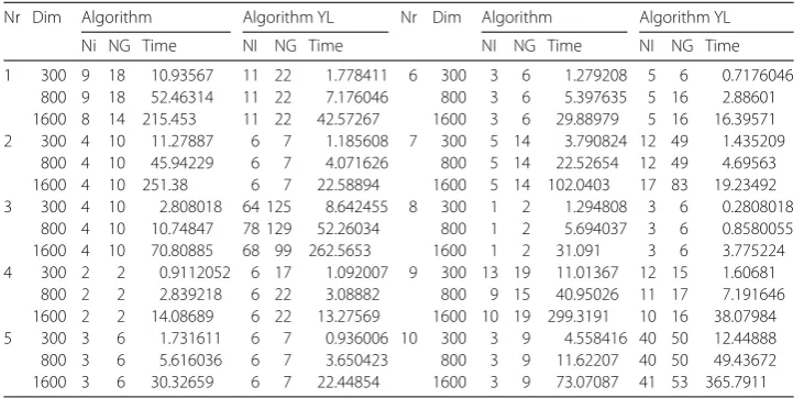
The column meaning in the following tables: Dim: the dimension. NI: the number of iterations.
NG: the norm function number. Time: the CPU-time in seconds.
Numerical results of Table1show the performance of these two algorithms about NI, NG, and Time. It is not difficult to see that both of these algorithm can successfully solve all these ten nonlinear problems.
It is easy to see that the NI and the NG of Algorithm have won since their performance profile plot is on top right. And the Time of Algorithm YL has superiority over Algorithm. Both of these two algorithms have good robustness.
4 Conclusions
Table 1 Experiment results
Nr Dim Algorithm Algorithm YL Nr Dim Algorithm Algorithm YL
Ni NG Time NI NG Time NI NG Time NI NG Time
1 300 9 18 10.93567 11 22 1.778411 6 300 3 6 1.279208 5 6 0.7176046
800 9 18 52.46314 11 22 7.176046 800 3 6 5.397635 5 16 2.88601
1600 8 14 215.453 11 22 42.57267 1600 3 6 29.88979 5 16 16.39571
2 300 4 10 11.27887 6 7 1.185608 7 300 5 14 3.790824 12 49 1.435209
800 4 10 45.94229 6 7 4.071626 800 5 14 22.52654 12 49 4.69563
1600 4 10 251.38 6 7 22.58894 1600 5 14 102.0403 17 83 19.23492
3 300 4 10 2.808018 64 125 8.642455 8 300 1 2 1.294808 3 6 0.2808018
800 4 10 10.74847 78 129 52.26034 800 1 2 5.694037 3 6 0.8580055
1600 4 10 70.80885 68 99 262.5653 1600 1 2 31.091 3 6 3.775224
4 300 2 2 0.9112052 6 17 1.092007 9 300 13 19 11.01367 12 15 1.60681
800 2 2 2.839218 6 22 3.08882 800 9 15 40.95026 11 17 7.191646
1600 2 2 14.08689 6 22 13.27569 1600 10 19 299.3191 10 16 38.07984
5 300 3 6 1.731611 6 7 0.936006 10 300 3 9 4.558416 40 50 12.44888
800 3 6 5.616036 6 7 3.650423 800 3 9 11.62207 40 50 49.43672
1600 3 6 30.32659 6 7 22.44854 1600 3 9 73.07087 41 53 365.7911
the function involved being monotone. Based on the Phragmén–Lindelöf inequalities, the underlying system of inequalities was reformulated as a system of smooth equations, and a Schrödinger-type method was proposed to solve it iteratively so that a solution of the system of the Schrödinger equations was found. By means of the Schrödinger type in-equalities, the algorithm was proved to be well defined and to be globally convergent un-der weak assumptions and locally quadratically convergent unun-der suitable assumptions. Preliminary numerical results indicate that the algorithm was effective.
Acknowledgements
Not applicable.
Funding
Not applicable.
Abbreviations
Not applicable.
Availability of data and materials
Not applicable.
Competing interests
The author declares that she has no competing interests.
Authors’ contributions
The author read and approved the final manuscript.
Publisher’s Note
Springer Nature remains neutral with regard to jurisdictional claims in published maps and institutional affiliations.
Received: 12 February 2019 Accepted: 13 May 2019 References
1. Antoine, X., Besse, C., Klein, P.: Absorbing boundary conditions for general nonlinear Schrödinger equations. SIAM J. Sci. Comput.33, 1008–1033 (2012)
2. Bertsekas, D.P.: Nonlinear Programming. Athena Scientific, Belmont (1995)
3. Borzi, A., Decker, E.: Analysis of a leap-frog pseudospectral scheme for the Schrödinger equation. J. Comput. Appl. Math.193, 65–88 (2006)
4. Bratsos, A.G.: A modified numerical scheme for the cubic Schrödinger equation. Numer. Methods Partial Differ. Equ.
27, 608–620 (2011)
5. Gomez-Ruggiero, M., Martinez, J.M., Moretti, A.: Comparing algorithms for solving sparse nonlinear systems of equations. SIAM J. Sci. Stat. Comput.23, 459–483 (1992)
7. He, J., Zhang, X., Liu, L., Wu, Y., Cui, Y.: Existence and asymptotic analysis of positive solutions for a singular fractional differential equation with nonlocal boundary conditions. Bound. Value Probl.2018, Article ID 189 (2018) 8. Huang, J., Tao, X.: Weighted estimates on the Neumann problem for Schrödinger equations in Lipschitz domains.
Acta Math. Sci. Ser. A36(06), 1165–1185 (2016)
9. Kermack, W.O., M’Kendrick, A.D.: A contribution to the mathematical theory of epidemics. Proc. R. Soc. Lond. Ser. A
115, 700–721 (1997)
10. Ladde, G.S., Lakshmikatham, V.: Random Differential Inequalities. Academic Press, New York (1980) 11. Li, Y., Sun, Y., Meng, F., Tian, Y.: Exponential stabilization of switched time-varying systems with delays and
disturbances. Appl. Math. Comput.324, 131–140 (2018)
12. Liu, Z.: Existence results for the general Schrödinger equations with a superlinear Neumann boundary value problem. Bound. Value Probl.2019, Article ID 61 (2019)
13. Lu, Y., Kou, L., Sun, J., Zhao, G., Wang, W., Han, Q.: New applications of Schrödinger type inequalities in the Schrödingerean Hardy space. J. Inequal. Appl.2017, Article ID 306 (2017)
14. Ma, W.X., Zhou, Y.: Lump solutions to nonlinear partial differential equations via Hirota bilinear forms. J. Differ. Equ.
264(4), 2633–2659 (2018)
15. Nocedal, J., Wright, S.J.: Numerical Optimization. Springer, New York (1999)
16. Ortega, J.M., Rheinboldt, W.C.: Iterative Solution of Nonlinear Equations in Several Variables. Academic Press, New York (1970)
17. Qian, X., Chen, Y., Song, S.: Novel conservative methods for Schrödinger equations with variable coefficients over long time. Commun. Comput. Phys.15(3), 692–711 (2014)
18. Qiao, B., Ruda, H.: Generalized Schrödinger equation and quantum measurement. Phys. A355(2–4), 333–345 (2005) 19. Qiao, L., Tang, S., Zhao, H.: Single peak soliton and periodic cusp wave of the generalized Schrödinger–Boussinesq
equations. Commun. Theor. Phys.63(6), 731–742 (2016)
20. Raydan, M.: The Barzilai and Borwein gradient method for the large scale unconstrained minimization problem. SIAM J. Optim.7, 26–33 (1997)
21. Reichel, B., Leble, S.: On convergence and stability of a numerical scheme of coupled nonlinear Schrödinger equations. Comput. Math. Appl.55, 745–759 (2008)
22. Taniguchi, T.: Almost sure exponential stability for stochastic partial functional differential equations. Stoch. Anal. Appl.16(5), 965–975 (1998)
23. Wan, L.: Some remarks on Phragmén–Lindelöf theorems for weak solutions of the stationary Schrödinger operator. Bound. Value Probl.2015, Article ID 239 (2015)
24. Wang, Y., Liu, Y., Cui, Y.: Infinitely many solutions for impulsive fractional boundary value problem with p-Laplacian. Bound. Value Probl.2018, Article ID 94 (2018)
25. Wang, Y.J., Xiu, N.H.: Theory and Algorithm for Nonlinear Programming. Shanxi Science and Technology Press, Xian (2004)
26. Yan, Z., Park, J., Zhang, W.: A unified framework for asymptotic and transient behavior of linear stochastic systems. Appl. Math. Comput.325, 31–40 (2018)
27. Yuan, Y.: Trust region algorithm for nonlinear equations. Information1, 7–21 (1998)