The optical/X-ray connection: intra-cluster medium iron content
and galaxy optical luminosity in 20 galaxy clusters
T. F. Lagan´a,
1R. A. Dupke,
2L. Sodr´e Jr,
1G. B. Lima Neto
1and F. Durret
31Instituto de Astronomia, Geof´ısica e C. Atmosf./USP, R. do Mat˜ao 1226, 05508-090. S˜ao Paulo/SP, Brazil 2University of Michigan, Ann Arbor, MI 48109-1090, USA
3Institut d’Astrophysique de Paris, CNRS, UMR 7095, Universit´e Pierre et Marie Curie, 98bis Bd Arago, 75014 Paris, France
Accepted 2008 November 21. Received 2008 November 21; in original form 2008 August 13
A B S T R A C T
X-ray observations of galaxy clusters have shown that the intra-cluster gas has iron abundances of about one-third of the solar value. These observations also show that part (if not all) of the intra-cluster gas metals was produced within the member galaxies. We present a systematic analysis of 20 galaxy clusters to explore the connection between the iron mass and the total luminosity of early- and late-type galaxies, and of the brightest cluster galaxies (BCGs). From our results, the intra-cluster medium (ICM) iron mass seems to correlate better with the luminosity of the BCGs than with that of the red and blue galaxy populations. As the BCGs cannot produce alone the observed amount of iron, we suggest that ram-pressure plus tidal stripping acts together to enhance, at the same time, the BCG luminosities and the iron mass in the ICM. Through the analysis of the iron yield, we have also estimated that SN Ia are responsible for more than 50 per cent of the total iron in the ICM. This result corroborates the fact that ram-pressure contributes to the gas removal from galaxies to the ICM, being very efficient for clusters in the temperature range 2<kT(keV)<10.
Key words: galaxies: clusters: general – galaxies: evolution.
1 I N T R O D U C T I O N
The detection of the Fe line from the X-ray spectral analysis of the intra-cluster medium (ICM; Mitchell et al. 1976; Serlemitsos et al. 1977) indicates that it does not have a primordial chemical composition but was enriched with material processed in stars. The relative importance of the mechanisms that transport metal-rich gas to the ICM is not well known. The measurement of heavy element abundances in the ICM can provide important clues on the chemical evolution inside galaxy clusters.
Difficulties in determining the nature of metal enrichment in clusters are enhanced by the variety of astrophysical processes and spatial scales involved: yields from different supernova (SNe) types, the role of galactic winds (e.g. Dupke & White 2000), ram-pressure (e.g. Gunn & Gott 1972) and tidal stripping (e.g. Toomre & Toomre 1972) as mechanisms of metal transport from galax-ies to the ICM, star formation efficiency and the influence of the environment, among other issues.
An important step in clarifying this problem was taken by Arnaud et al. (1992). These authors investigated the correlations between some properties of the ICM, like the gas mass, with the optical lu-minosity in clusters, finding that the gas mass correlates well with the luminosity of E+S0 galaxies but not with the luminosity of
E-mail: [email protected]
spirals. For a sample of six clusters with measured iron abundances and at low redshift, they also found a good correlation between the iron mass and the luminosity of red galaxies (E+S0). They then concluded that ellipticals and lenticulars are dominant in enriching the ICM, indicating that the protogalactic winds driven by Type II SNe at the early stages of cluster formation play a major role in the ICM metal enrichment. Another relevant enrichment mechanism is ram-pressure stripping (hereafter RPS; Gunn & Gott 1972). Current observations indicate that RPS is more common than previously be-lieved, acting also in low-density environments such as poor groups and in the outskirts of clusters (Solanes et al. 2001; Kantharia et al. 2005; Levy et al. 2007; Kantharia, Rao & Sirothia 2008). This is also supported by recent numerical simulations (e.g. Vollmer, Huchtmeier & van Driel 2005; Hester 2006; Br¨uggen & De Lucia 2008). Ram-pressure-stripped gas is more enriched by SN Ia ejecta and can continuously provide an inflow of iron to the ICM through the cluster history (Renzini et al. 1993).
Table 1. Clusters from Maughan et al. (2008) data sample which were observed by SDSS and have X-ray flux high enough for the analysis presented here. Column (1): cluster name; col. (2): right ascension; col. (3): declination; col. (4): redshift; col. (5):r500radius; col. (6): mean
temperature derived from the X-ray emission withinr500; col. (7): mean metallicity inside withinr500; col. (8): gas mass withinr500.
Cluster RA Dec. z r500 kT Z Mgas
(J2000) (J2000) (h−701) Mpc (keV) 1013M
A267 01:52:42.12 +01:00:41.4 0.230 1.04 4.9−+00..33 0.49+
0.18
−0.17 5.74+ 0.10 −0.07
MS0906.5+1110 09:09:12.72 +10:58:33.6 0.180 1.06 5.3+−00..22 0.31+−00..0707 5.27+−00..0504 A773 09:17:52.80 +51:43:40.4 0.217 1.25 7.4+−00..33 0.48−+00..0606 9.09+−00..0606 MS1006.0+1202 10:08:47.52 +11:47:40.6 0.221 1.11 5.9+−00..44 0.16+−00..1010 5.29+−00..0606 A1204 11:13:20.40 +17:35:39.1 0.171 0.92 3.4+0−0..11 0.37−+00..0505 3.10+0−0..2106 A1240 11:23:37.68 +43:05:44.5 0.159 0.92 3.9+−00..33 0.19−+00..1009 2.75+−00..0403 A1413 11:55:18.00 +23:24:17.6 0.143 1.26 7.2+−00..22 0.41−+00..0303 7.95+−00..0405 A1682 13:06:51.12 +46:33:29.5 0.234 1.13 6.2+0−0..88 0.42−+00..2725 7.07+0−0..1312 A1689 13:11:29.52 −01:20:30.4 0.183 1.37 9.0+−00..33 0.42−+00..0404 11.26+−00..1106 A1763 13:35:18.24 +40:59:59.3 0.223 1.32 7.8+−00..44 0.29−+00..0707 11.47+−00..1007 A1914 14:26:01.20 +37:49:35.4 0.171 1.37 9.8+−00..33 0.34−+00..0505 10.69+−00..0907 A1942 14:38:22.08 +03:40:06.2 0.224 0.94 4.3+−00..32 0.27−+00..0808 3.59+−00..0303 RXJ1504−0248 15:04:07.44 −02:48:18.4 0.215 1.34 6.8+−00..22 0.35+−00..0404 10.9+−00..0447 A2034 15:10:12.48 +33:30:28.4 0.113 1.22 6.7+0−0..22 0.38+0−0..0404 6.88+0−0..0203 A2069 15:24:09.36 +29:53:10.0 0.116 1.20 6.3+−00..22 0.29−+00..0505 6.56+−00..0303 A2111 15:39:41.28 +34:25:10.2 0.229 1.18 6.8+0−0..95 0.23−+00..1515 7.44+0−0..1005 RXJ1701+6414 17:01:23.04 +64:14:11.4 0.225 0.93 5.2+−00..64 0.60+−00..1817 4.21+−00..02806 A2259 17:20:08.64 +27:40:09.8 0.164 1.09 5.6+−00..44 0.28−+00..1110 5.29+−00..0807 RXJ1720.1+2638 17:20:10.08 +26:37:29.3 0.164 1.24 6.1+0−0..11 0.48+0−0..0303 7.46+0−0..3101
RXJ2129.6+0005 21:29:40.08 +00:05:19.6 0.235 1.20 5.6+0−0..33 0.50+0−0..1010 8.02+0−0..1414
there are currently a number of studies providing ICM physical parameters from large cluster samples homogeneously determined (e.g. Zhang et al. 2007; Maughan et al. 2008).
To readdress this question, we investigate in this work the relation between the metallicity (iron abundance) of the intra-cluster gas and some optical properties of galaxy clusters, in search for clues on how metals got into the ICM.
The outline of the paper is as follows. In Section 2, we describe the sources of the data analysed. In Section 3, we present the photo-metric analysis, describing the separation between the red and blue populations and the determination of their total luminosity. The in-fluence of the Butcher–Oemler (BO) effect is also discussed in this section. In Section 4, we discuss the dominant population in the iron enrichment by means of the correlation between the iron mass and the total luminosity of the different populations, the mechanism responsible for the metal transport from galaxies to the ICM and the role of SN II and SN Ia. Finally, we present our conclusions in Section 5.
2 T H E D ATA
We describe in this section the X-ray and optical data used in our analysis.
2.1 X-ray Data
Maughan et al. (2008) carried out an X-ray analysis of a homo-geneous sample of 115 galaxy clusters in the redshift range 0.1<
z<1.3. The sample was assembled from publicly available Chan-dradata and selected in order to ensure cluster emission detection up tor500(the radius within which the cluster mean density exceeds
the critical value by a factor of 500), allowing cluster properties to be directly measured up to this radius. We have selected a subsam-ple of galaxy clusters that were analysed by Maughan et al. (2008) and observed by theSloan Digital Sky Survey(SDSS; York et al. 2000). Out of 115 clusters, 20 were selected (Table 1), and will be the object of the analysis presented in this paper. All the X-ray data used here (metallicity, gas mass and temperature) are taken from Maughan et al. (2008) and are also presented in Table 1.
In order to check if the 20 clusters analysed in this work are a fair sample of the original one, we present in Fig. 1 the metallicity (iron abundance) for all the clusters studied by Maughan et al. (2008). The mean metallicity value [Z=(0.34±0.15) Z] obtained for our selected subsample agrees well with the mean value [Z=(0.39± 0.14) Z] obtained for the original 115 clusters.
2.2 SDSS data
The photometric data used in our analysis come from SDSS Data Release 5 (DR5; Adelman-McCarthy et al. 2007), which contains spectroscopic and photometric data for a large number of galaxies observed within almost a quarter of the sky.
Figure 1.Distribution of iron abundance determined withinr500 for our
selected subsample (in dark blue) and for the whole sample analysed by Maughan et al. (2008) (filled with dashed lines). Our mean value isZ= (0.34±0.15) Z, while the average mean for the whole sample isZ= (0.39±0.14) Z.
of each cluster centre (adopted as the X-ray centre from Maughan et al. 2008). This magnitude limit ensures a significant number of objects for the galaxy population analysis. In this study, we will adopt the (g−r) colour, from the DERED tables which are tables of magnitudes already corrected for galactic extinction.
We have also downloaded the same type of data in an annular control field around each cluster (see Section 3), for the statistical subtraction of foreground/background galaxies.
3 P H OT O M E T R I C A N A LY S I S
Since the number of galaxies with measured redshifts in the field of each cluster is small, we have adopted a statistical approach, based on the analysis of the colour–magnitude diagram (CMD) of each cluster, to estimate some properties of the cluster galaxies.
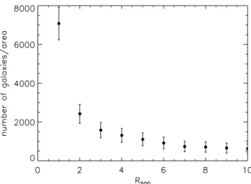
We present in Fig. 2 the (g−r) versusrCMD of A2034 for all galaxies withinr500. Early-type galaxies in clusters present a tight
Figure 2.Colour–magnitude diagram for galaxies insider500for A2034,
divided in the three groups discussed in the text: red, blue and background galaxies.
correlation between their optical colours and luminosity, known as colour–magnitude relation or red sequence (RS), which is very use-ful for their identification. In general, galaxies significantly above the RS are in the cluster background (since they are redder than the reddest cluster galaxies). We call those galaxies below the RS as blue galaxies (see Fig. 2), which comprise clusters and non-clusters members.
We have used the control fields to obtain the field contamination and the correction required to estimate the numbers and luminosities of cluster galaxies. The procedure we adopt is the following: the first step is to determine, for each field, the position of the RS. Bower, Lucey & Ellis (1992), Gladders et al. (1998) and Romeo et al. (2008), among others, have shown that the slope of the RS in CMDs is almost constant up to redshiftz=0.5. For this reason, given that all clusters in our sample have redshifts well below this value, we assume that this slope is the same for all clusters in Table 1. Thus, we have used the CMDs of the five clusters of our sample (MS0906.5+1110, A2034, A2069, A2259 and RXJ1720.1+2638) with the most prominent RS to estimate this slope through a linear fit, obtaining∼ −0.055 (g−r)/r(see Fig. 2).
For all clusters, we fitted the RS as a function ofr-band magnitude according to
(g−r)= −0.055r+A (1)
to obtain the zero-point coefficient (A). Then, in each cluster, we divided the galaxies in three groups.
(i)Red galaxies: those galaxies within 0.3 mag (De Lucia & Poggianti 2008) from the best-fitting colour–magnitude relation. That is (g−r)±0.3 mag zone.
(ii) Blue galaxies: galaxies bluer than the (g−r)−0.3 mag. This group contains mainly star-forming galaxies, both in the cluster and in the field.
(iii)Background galaxies: galaxies redwards of the upper limit of the RS. We assume that these galaxies are not cluster members.
We estimate the cluster contamination by background/foreground galaxies using a control field around the cluster defined as an annular region between 7 ×r500 and 8 ×r500 from the cluster centre.
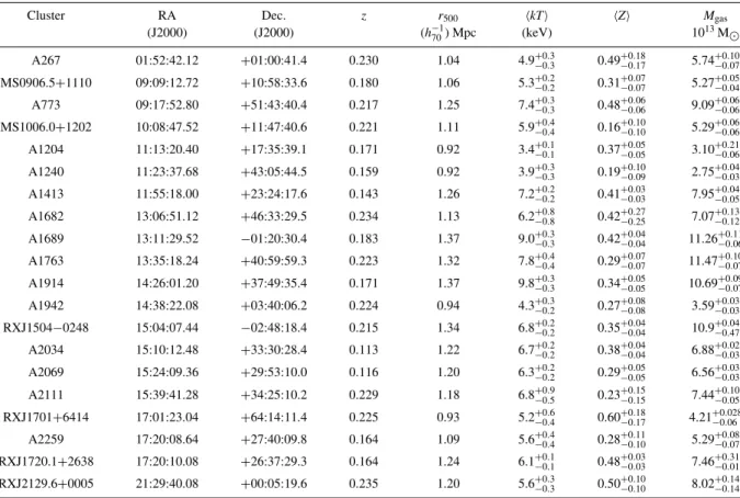
This region is far enough from the centre to allow the estimation of background densities, as shown in Fig. 3. We used the CMDs of the galaxies in the control fields to estimate the background
Figure 3. Galaxy counts distribution as a function of the mean radius of each annulus, given as a function ofr500, for A1689. The background is
Figure 4. Colour–magnitude diagrams withinr500for the 20 clusters in our sample.
contamination (in the number of galaxies and luminosity) for red and blue galaxies in the cluster. The CMDs for the clusters in our sample are shown in Fig. 4.
For each bin of magnitude, the number count of galaxies is given by
Ncl(m)=Ncl+bkg(m)−γ Nbkg(m), (2)
whereNcl(m) is the expected number of cluster galaxies at a
cer-tain magnitude interval,Ncl+bkg(m) is the total number of galaxies
along the line of sight in the same magnitude interval,Nbkg(m) is
the number of background and foreground galaxies in the same magnitude interval,γis the ratio between cluster and control field areas andmis the mean magnitude of the interval. After subtract-ing the background and foreground contamination, cluster counts per magnitude bin in therband were determined and converted to luminosity.
3.1 Luminosity of the brightest galaxies
The division of our sample in groups described above enables us to separately calculate the total luminosity of the red and the blue pop-ulation. We obtained ther-band luminosity of the brightest cluster galaxies (BCGs),LBCG, directly from the SDSS.
We used the distance modulus given by
Mr =mr−25−5 log(dL/1 Mpc)−k(z), (3)
where dL is the luminosity distance (computed assuming m =
0.3, λ = 0.7 and h= 0.7) and k(z) is the k-correction
com-puted by Poggianti (1997). Converting magnitudes to luminosities, we integrated the luminosity function in order to obtain the total luminosity for each population. These luminosities are given in Table 2.
Table 2. Properties derived from optical data. Column (1): cluster name; col. (2): total luminosity of the red population withinr500; col. (3): total
luminosity of the blue population withinr500; col. (4): luminosity of BCGs;
col. (5): iron mass derived from equation (4) withinr500.
Cluster Lred Lblue LBCG MFe
(1012L) (1012L) (1011L) (1011M) A267 2.19±0.03 1.82±0.01 1.84 0.52±0.18 MS0906.5+1110 2.69±0.05 1.00±0.01 0.92 0.30±0.06 A773 3.82±0.07 2.08±0.01 0.68 0.80±0.10 MS1006.0+1202 1.85±0.05 1.45±0.01 1.22 0.16±0.09 A1204 0.66±0.02 0.74±0.02 0.54 0.21±0.03 A1240 0.79±0.02 0.73±0.07 0.13 0.10±0.05 A1413 0.79±0.04 0.83±0.01 1.71 0.60±0.04 A1682 2.9±0.08 2.34±0.02 0.94 0.54±0.32 A1689 2.31±0.04 1.21±0.07 0.76 0.87±0.01 A1763 3.21±0.02 2.18±0.03 0.83 0.61±0.02 A1914 1.77±0.03 0.92±0.04 0.46 0.67±0.09 A1942 2.22±0.08 1.44±0.01 0.89 0.18±0.05 RXJ1504−0248 1.66±0.04 1.35±0.08 1.66 0.70±0.05 A2034 0.53±0.02 0.35±0.06 0.87 0.48±0.05 A2069 0.89±0.04 0.34±0.04 0.41 0.35±0.06 A2111 4.16±0.02 2.06±0.02 0.54 0.31±0.20 RXJ1701+6414 2.02±0.05 1.59±0.01 0.06 0.46±0.16 A2259 0.92±0.05 1.02±0.07 1.22 0.27±0.09 RXJ1720.1+2638 1.13±0.03 0.94±0.07 1.23 0.66±0.38 RXJ2129.6+0005 2.15±0.01 2.08±0.02 1.15 0.73±0.14
3.2 Butcher–Oemler effect
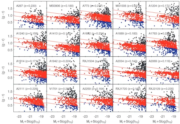
Figure 5.Spiral fraction as a function of redshift. The dashed line is our best fit for this sample. The filled circles are the sample analysed in this work, while the green points were taken from Rakos & Schombert (1995) and the upside down blue triangles are taken from Margoniner & de Carvalho (2000) for this redshift interval.
environment of galaxy clusters, most of their interstellar medium (ISM) gas ends up being transferred to the ICM, contributing to its chemical enrichment. We call attention to the fact that the time-scale of colour (spectral) evolution is shorter than that of the morpholog-ical evolution (Goto et al. 2004), meaning that some passive spiral galaxies through their evolution may be observed as red objects.
An observational evidence of the hierarchical scenario is the BO effect (Butcher & Oemler 1984). We have noted that this effect can be detected with our data (and has been previously detected by Rakos & Schombert 1995; Margoniner & de Carvalho 2000), and Fig. 5 shows that this trend can be detected even in low-redshift clusters. We define the fraction of blue galaxies as the ratio between the number of blue galaxies (see Section 3) and the total number of galaxies in a cluster after background correction, indicating an extremely rapid change in the fraction of blue galaxies from∼10 to more than 30 per cent at onlyz∼0.25. In contrast, evolutionary models for passive evolution of simple stellar populations predict that colour changes were not as dramatic as found here (Rakos & Schombert 1995).
4 T H E I R O N C O N T E N T / O P T I C A L L I G H T C O N N E C T I O N I N 2 0 G A L A X Y C L U S T E R S
In this section, we investigate the links between the iron content and the luminosities of the red and blue populations of each cluster.
4.1 The iron mass and its relation to the luminosity of the galaxy populations withinr500
In clusters, there are a number of emission lines over the continuum bremsstrahlung spectrum, the most prominent being those in the iron complex at∼7 keV. X-ray observations have revealed the presence of heavy elements in the ICM, providing direct evidence that this gas was enriched by metals processed by stars (e.g. Mitchell et al. 1976; David, Forman & Jones 1991; Mushotzky et al. 1996). Studies of large samples of clusters have shown that the Fe abundance is distributed around a value of 0.3 solar (Mushotzky & Loewenstein 1997; Allen & Fabian 1998; Tozzi et al. 2003; Ettori 2005), which is consistent with the mean value of our sample,Z=0.34±0.15.
The metallicity derived from X-ray spectra is emission-weighted, so that the values from the central regions tend to overpower global spectral fittings. Therefore, a single global abundance value may lead to erroneous results when associating metals to galaxy lumi-nosities in the whole cluster.Chandra’s excellent spatial resolution is greatly advantageous over previous satellites for this analysis for intermediate-redshift clusters because it can separate the inner and outer regions extremely well (not including projection effects), so that accurate average abundances out of the cooling core region can be measured, making our analysis more realistic. While Arnaud et al. (1992) used one single value for abundances, we are using two different values (one for the internal regions, within 0.15r500,
and the other for the annulus 0.15r500<r<r500), and the results
are very similar (Section 4.2). Naturally, one single value for the outer abundances is still susceptible to the above-mentioned biases, but there were simply not enough photons to subdivide the outer regions in several annuli and still have abundances with satisfactory significance.
In the present work, the iron mass of each cluster enclosed within
r500was estimated as the product of the iron abundance by the gas
mass and by the solar photospheric abundance by mass (0.00197; Anders & Grevesse 1989)
MFe=Mgas(< r500)×Z×0.00197, (4)
whereMgasis the gas mass andZis the metallicity, both computed
withinr500.
Equation (4) gives the relation between the iron mass in the ICM and the gas mass for our sample. The iron mass is consistent with a linear scaling with the gas mass, which is expected if ZFe ≈
constant.
To explore what is the dominant population responsible for the metal enrichment in galaxy clusters, we show, in Fig. 6, the de-pendence of the iron mass with the luminosity of red, blue and BCG galaxies. Given the large scatter observed, we adopt the ro-bust Spearman correlation coefficient ρ and the null probability (NP; i.e. the probability of failing to reject the null hypothesis) to evaluate the significance of the correlations (see Press et al. 1992). We obtainρvalues equal to 0.021 (NP=92 per cent), 0.15 (NP= 52 per cent) and 0.41 (NP=8 per cent) for the red, blue and BCG galaxies, respectively. The statistical significance of the correlations between luminosities of different populations and ICM iron mass is very low, as seen in Fig. 6. Fig. 6 shows that all the correlations are very poor and it is not obvious that a given galaxy population is more significantly correlated with the iron mass than the others. To address this question, we adopted a bootstrap resampling technique to estimate for what fraction of a sample a correlation is better than another in the sense that it has a larger Spearman rank-order coef-ficientρ(Press et al. 1992). We found that the correlation between the iron mass and BCG luminosities is better than that with the luminosities of the red galaxies at the 90 per cent confidence level and of the blue population at the 85 per cent confidence level. We also found that the significance of the correlations between the blue and red populations with iron mass is barely distinguishable and, in consequence, we cannot draw any firm conclusion about the relative importance of these two populations in the ICM iron enrichment.
Figure 6. Left-hand panel: iron content as a function of total luminosity for red galaxies. Middle panel: iron content as a function of total luminosity for blue galaxies. Right-hand panel: iron content as a function of BCG luminosities. The regression line has a slope ofα=0.75. The 1σerror onαis±0.33.
between the iron mass and the BCGs luminosities. Note that their best fit for the iron mass as a function of the ‘E+S0’ luminosities has a slope ofα=1.0±0.25, which is, given the uncertainties, con-sistent with the poor correlation obtained here between the BCGs and the iron mass. Including the BCGs in the sample of red galaxies changes the correlation coefficient between the total galaxy lumi-nosity and the iron mass fromρ=0.021 to 0.31, closer to that found for BCGs alone, as expected for the case of contamination by the BCGs.
Since the iron mass scales with the gas mass and with the Fe abundance, we separately plot the relations between the metallicities (see upper panels of Fig. 7) and gas masses (see bottom panels of Fig. 7) versus the optical galaxy luminosities. From these figures, we still have low statistical correlations but the ones between the BCGs luminosities and either the gas mass or the metallicity are somewhat more visible than the others. We obtained correlation coefficients equal toρ=0.075,ρ=0.17 andρ=0.26 for the metallicity and the luminosities of the red, blue and BCGs galaxies, respectively. For the correlations between the gas mass and the luminosities, we obtainedρ=0.31,ρ=0.21 andρ=0.33 for the red, blue and BCG population, respectively. The slightly better correlation of gas mass withLred(as opposed toLblue) is consistent with the enhancement
of the fraction of elliptical galaxies with richness (Dressler 1980), given the somewhat high-temperature range of our sample (T > 3.4 keV).
4.2 The iron mass and its relation with the luminosity of the galaxy populations within an external annulus
De Grandi et al. (2004) found that the iron mass associated to abundance excess, which is normally found at the centre of cool-core clusters, can be entirely produced by the BCGs. In order to take into account possible biases due to contamination by cool-core processes, we present here the same correlations computed within an external annulus, (0.15–1)r500, to exclude the inner parts.
The iron mass of each cluster enclosed within (0.15<r<1)R500
was estimated from equation (4) and the gas mass was computed as
Mgas=
r500
0.15r500
ρg4πr2dr =4π mHZ
r500
0.15r500
ne(r)r2dr, (5)
whereZ=1.25 is the mean atomic weight for a H+He plasma,
mHis the hydrogen mass andne(r) is the electron density which was
fitted with a modified version of the standardβ-model (as proposed by Vikhlinin et al. 2006, withγ=3 fixed for all fits). The best-fitting parameters were taken from Maughan (private communication). In Table 3, we present the values for the iron mass for our sample.
We show in Fig. 8 the plots between the iron mass and the lu-minosity of red, blue and BCG galaxies within (0.15–1)r500. We
obtainedρvalues equal to 0.15 (NP=48 per cent), 0.16 (NP= 49 per cent) and 0.41 (NP=17 per cent) for the correlation between the iron mass and red, blue and BCG galaxies, respectively. Hence, we verified that even excluding the central region, where we could find an iron excess due to the BCGs (De Grandi et al. 2004), the iron mass present in the ICM seems to still correlate better with the BCG population. In the next section, we discuss a possible scenario to explain this dependence.
4.3 The source of ICM metals
The plots obtained in Figs 6 and 8 suggest that the BCGs could play a significant role in the ICM iron enrichment. The most parsimonious scenario is that a mechanism simultaneously contributes to enhance the metal mass and the luminosity of the BCG. Such a mechanism can be, for example, RPS with tidal disruption of the galaxy near the centre of the cluster (e.g. Cypriano et al. 2006; Murante et al. 2007).
RPS can be a significant contributor to metal injection in the ICM. From the theoretical side, the ISM of galaxies will be stripped if the ICM density is as low as 5×10⁻⁴ atoms cm−3 (Gunn &
Gott 1972). This rough estimate (other factors, such as the direction along which the galaxy is travelling through the ICM, may affect this number) suggests that RPS could be effective at large spatial scales in most galaxy clusters (Tonnesen & Bryan 2008).
Figure 7.Upper panels: Fe abundance withinr500as a function of the total luminosity of the red galaxies (left-hand panel), total luminosity of the blue
galaxies (middle panel) and as a function of the BCG luminosities (right-hand panel). Bottom panels: gas mass as functions of the total luminosity of the red galaxies (left-hand panel), total luminosity of the blue galaxies (middle panel) and the BCG luminosities. We do not find any significant trend in these panels.
in principle, play a significant role. Using hydrodynamical simu-lations to study RPS, McCarthy et al. (2008) found that∼70 per cent of the galactic halo is stripped for typical structural and orbital parameters.
If RPS is important and has a dependence on cluster mass we should see a trend between gas temperature and metallicity, since the higher the mass (or the temperature) the more metals are stripped from galaxies and injected into the ICM. However, we do not see this trend (Fig. 9) within the temperature range of our sample [2<
kT (keV)<10]. Therefore, either RPS is negligible, which con-tradicts the theoretical expectations and the observations described in the previous paragraphs, or RPS is equally significant for all clusters, once the threshold ICM density is reached. Since RPS is not biased by galaxy morphology, this would be consistent with the lack of a correlation between iron mass and galaxy morphology.
Chemical evolution models have been invoked to analyse the iron metallicity, suggesting that the number of SN Ia that ever occurred relative to SN II isNIa/NII=0.12, with more than 50 per cent of
the56Fe mass coming from SN Ia (Yoshii, Tsujimoto & Nomoto
1996; Nomoto et al. 1997). The iron yield (p) is given by (Arnaud et al. 1992)
[MFe]ICM+[MFe]≤pM, (6)
where the two terms in the left-hand side are the total iron mass in the ICM, [MFe]ICM, and in stars, [MFe], andMis the total stellar
mass. Since the ratio ([MFe]ICM +[MFe])/Mcannot exceed the
iron yield, if we assume that all the iron ever produced goes to the ICM, we have
[MFe]ICM
M
≤p, (7)
that is,MFe/Mgives an upper limit for the iron yield, since some
recycling must have occurred.
The total mass in stars can be computed by multiplying the to-tal luminosity (Lred+Lblue) by an appropriate mass-to-light ratio.
The late- and early-type mass-to-light ratios were estimated from Kauffmann et al. (2003) and converted to the r band accord-ing to Fukugita, Shimasaku & Ichikawa (1995), and areM/L=
3.27 M/Lfor a red population andM/L=1.64 M/Lfor a blue population. This procedure is explained in details in Lagan´a et al. (2008).
For our sample, the mean iron-to-stellar mass ratio is [MFe]ICM/M=(6.0±0.5)×10−3. David, Forman & Jones (1990)
calculated the amount of iron that type II driven winds can inject in the ICM. These authors obtained [MFe]ICM/Mranges from 0.65×
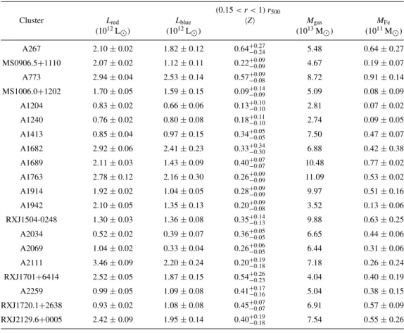
Table 3. Properties derived from optical data. Column (1): cluster name; col. (2): total luminosity of the red population inside (0.15–1)r500; col. (3): total luminosity of the blue population inside (0.15–1)r500; col. (4): luminosity of BCGs;
col. (5): iron mass derived from equation (4) within (0.15–1)r500.
(0.15<r<1)r500
Cluster Lred Lblue Z Mgas MFe
(1012L
) (1012L
) (1013M
) (1011M
)
A267 2.10±0.02 1.82±0.12 0.64−0+0..2724 5.48 0.64±0.27 MS0906.5+1110 2.07±0.02 1.12±0.11 0.22−0+0..0909 4.67 0.19±0.07 A773 2.94±0.04 2.53±0.14 0.57+−00..0908 8.72 0.91±0.14 MS1006.0+1202 1.70±0.05 1.59±0.15 0.09−+00..1409 5.09 0.08±0.09 A1204 0.83±0.02 0.66±0.06 0.13+−00..1010 2.81 0.07±0.02 A1240 0.76±0.02 0.80±0.08 0.18−0+0..1110 2.74 0.09±0.05 A1413 0.85±0.04 0.97±0.15 0.34+−00..0505 7.50 0.47±0.07 A1682 2.92±0.06 2.41±0.23 0.33+−00..3430 6.88 0.42±0.38
A1689 2.11±0.03 1.43±0.09 0.40−0+0..0707 10.48 0.77±0.02 A1763 2.78±0.12 2.16±0.30 0.26−0+0..0909 11.09 0.53±0.02 A1914 1.92±0.02 1.04±0.05 0.28+−00..0909 9.97 0.51±0.16 A1942 2.10±0.05 1.35±0.13 0.20+−00..0908 3.52 0.13±0.06 RXJ1504-0248 1.30±0.03 1.36±0.08 0.35+−00..1413 9.88 0.63±0.25
A2034 0.52±0.02 0.39±0.07 0.36+−00..0505 6.65 0.44±0.06 A2069 1.04±0.02 0.33±0.04 0.26+−00..0605 6.44 0.31±0.06 A2111 3.46±0.09 2.20±0.24 0.20−0+0..1918 7.18 0.26±0.24 RXJ1701+6414 2.52±0.05 1.87±0.15 0.54−+00..2623 4.04 0.40±0.19 A2259 0.99±0.05 1.09±0.08 0.41+−00..1716 5.04 0.38±0.15 RXJ1720.1+2638 0.93±0.02 1.08±0.08 0.45−+00..0707 6.91 0.57±0.09 RXJ2129.6+0005 2.42±0.09 1.95±0.14 0.40−+00..1918 7.54 0.55±0.26
Figure 8. Correlations between the total luminosities and the iron mass within (0.15–1)r500. Left-hand panel: iron content as a function of the total luminosity
of the red galaxies. Middle panel: iron content as a function of the total luminosity of the blue galaxies. Right-hand panel: iron content as a function of the BCG luminosities.
assumption. Our results show much higher values suggesting that more than 50 per cent of the iron present in the ICM is probably produced in SN Ia. Most of the iron produced by SN Ia is preferen-tially injected into the ICM by RPS. Since RPS is equally efficient within the temperature range of our sample, the suggestion that more than half of the iron mass is produced in Type Ia SN
corrob-orates the result of a lack of trend between the metallicity and the ICM temperature.
Figure 9. Metallicity as a function of temperature for the clusters analysed in this work. The dashed line represents the mean value of the iron abundance in this sample.
for part of the iron found in the ICM, followed by a secondary phase, associated to the BCG formation, contributing with more than 50 per cent of the ICM iron, where most of the metals were produced by SN Ia and injected in the ICM by RPS.
5 C O N C L U S I O N S
We have carried out a detailed analysis of the iron mass in the ICM and its correlation with optical properties for 20 galaxy clusters previously studied by Maughan et al. (2008) and available in the SDSS. Our main results are as follows.
(i) We could not confirm a previous correlation between the ICM iron mass and the total luminosity of the red population, found by Arnaud et al. (1992). Since our results indicate that the BCGs seem to play a major role in the ICM iron enrichment, we suggest that the trend found by Arnaud et al. (1992) is biased by the BCGs as these authors did not exclude them from the ‘E+S0’ population. As the BCGs alone cannot produce the observed metallicity within
r500, we explain the correlation between the iron mass and the BCG
luminosities through a scenario in which a mechanism simultane-ously enhances the luminosity of the BCG and the iron mass in the ICM. We suggest RPS with tidal disruption near the cluster cen-tre as a possible mechanism, the importance of which is supported by recent hydrodynamical simulations (mechanism III of Murante et al. 2007).
(ii) The lack of trend between the iron metallicity and the cluster temperature indicates that RPS is equally efficient in all clusters within the range 2<kT (keV)<10. This is in agreement with current observational and theoretical (Tonnesen & Bryan 2008) studies, which suggest that RPS is more common in low-density environments than previously thought. Thus, RPS is a significant mechanism for transferring iron from galaxies to the intra-cluster gas.
(iii) The comparison of our results with predictions of chemical evolution models suggests that more than 50 per cent of the iron has come from Type Ia SNe. Since most of the iron produced by SN Ia is preferentially injected into the ICM by RPS, the iron yield corroborates the efficiency of RPS within the temperature range of this sample analysed here. There have been observational evidence, supported by hydrodynamical simulations, that the RPS mechanism
is contributing to the gas removal from galaxies that merged to form the BCGs (Murante et al. 2007).
(iv) We suggest that the complex history of galaxy populations in clusters, from galaxy infall followed by the action of severe environmental effects, leads to galaxy morphological (and colour) evolution and, at the same time, to a progressive enrichment of the ICM, diluting the role of any single population. Clearly, larger samples are needed to verify if these correlations are actually real.
AC K N OW L E D G M E N T S
The authors thank B. J. Maughan for making available the best-fitting parameters of the density profiles and the anonymous ref-eree for constructive suggestions. The authors also acknowledge financial support from the Brazilian agencies FAPESP, CNPq and CAPES (grants: 03/10345-3 and BEX1468/05-7), as well as the Brazilian–French collaboration CAPES/Cofecub (444/04). R. Dupke acknowledges partial support from NASA (grants: GO5-6139X, NNX06AG23G, NNX07AH55G and NNX07AQ76G). We also wish to thank the team of the SDSS for their dedication to a project which has made the present work possible.
R E F E R E N C E S
Adelman-McCarthy J. K. et al., 2007, ApJS, 172, 634 Allen S. W., Fabian A. C., 1998, MNRAS, 297, L63
Anders E., Grevesse N., 1989, Geochimica Cosmochimica Acta, 53, 197 Arnaud M., Rothenflug R., Boulade O., Vigroux L., Vangioni-Flam E., 1992,
A&A, 254, 49
Bower R. G., Lucey J. R., Ellis R. S., 1992, MNRAS, 254, 601
Bravo-Alfaro H., Cayatte V., van Gorkom J. H., Balkowski C., 2000, AJ, 119, 580
Br¨uggen M., De Lucia G., 2008, MNRAS, 383, 1336 Butcher H., Oemler A. Jr, 1984, ApJ, 285, L426
Cypriano E. S., Sodr´e L. J., Campusano L. E., Dale D. A., Hardy E., 2006, AJ, 131, 2417
David L. P., Forman W., Jones C., 1990, ApJ, 359, 29 David L. P., Forman W., Jones C., 1991, ApJ, 380, 39
De Grandi S., Ettori S., Longhetti M., Molendi S., 2004, A&A, 419, 7 De Lucia G., Poggianti B. M., 2008, ASP Conf. Ser., 399, 314 Dressler A., 1980, ApJ, 236, 351
Dupke R. A., White R. E. III, 2000, ApJ, 528, 139
Elbaz D., Arnaud M., Vangioni-Flam E., 1995, A&A, 303, 345 Ettori S., 2005, MNRAS, 362, 110
Fukugita M., Shimasaku K., Ichikawa T., 1995, PASP, 107, 945
Gladders M. D., Lopez-Cruz O., Yee H. K. C., Kodama T., 1998, ApJ, 501, 571
Goto T., Yagi M., Tanaka M., Okamura S., 2004, MNRAS, 348, 515 Gunn J. E., Gott J. R. I., 1972, ApJ, 176, 1
Haynes M. P., Giovanelli R., Chincarini G. L., 1984, ARA&A, 22, 445 Hester J. A., 2006, ApJ, 647, 910
Kantharia N. G., Ananthakrishnan S., Nityananda R., Hota A., 2005, A&A, 435, 483
Kantharia N. G., Rao A. P., Sirothia S. K., 2008, MNRAS, 383, 173 Kauffmann G. et al., 2003, MNRAS, 341, 33
Lagan´a T. F., Lima Neto G. B., Andrade-Santos F., Cypriano E. S., 2008, A&A, 485, 633
Levy L., Rose J. A., van Gorkom J. H., Chaboyer B., 2007, AJ, 133, 1104 Margoniner V. E., de Carvalho R. R., 2000, AJ, 119, 1562
Matteucci F., Gibson B. K., 1995, A&A, 304, 11
Maughan B. J., Jones C., Forman W., Van Speybroeck L., 2008, ApJS, 174, 117
Mitchell R. J., Culhane J. L., Davison P. J. N., Ives J. C., 1976, MNRAS, 175, 29P
Murante G., Giovalli M., Gerhard O., Arnaboldi M., Borgani S., Dolag K., 2007, MNRAS, 377, 2
Mushotzky R. F., Loewenstein M., 1997, ApJ, 481, L63
Mushotzky R., Loewenstein M., Arnaud K. A., Tamura T., Fukazawa Y., Matsushita K., Kikuchi K., Hatsukade I., 1996, ApJ, 466, 686 Nomoto K., Iwamoto K., Nakasato N., Thielemann F.-K., Brachwitz F.,
Tsujimoto T., Kubo Y., Kishimoto N., 1997, Nucl. Phys. A, 621, 467 Poggianti B. M., 1997, A&AS, 122, 399
Press W. H., Teukolsky S. A., Vetterling W. T., Flannery B. P., 1992, Nu-merical Recipes in FORTRAN. The Art of Scientific Computing, 2nd edn. Cambridge Univ. Press, Cambridge
Rakos K. D., Schombert J. M., 1995, ApJ, 439, 47
Renzini A., Ciotti L., D’Ercole A., Pellegrini S., 1993, ApJ, 419, 52 Romeo A. D., Napolitano N. R., Covone G., Sommer-Larsen J.,
Antonuccio-Delogu V., Capaccioli M., 2008, MNRAS, 389, 13
Serlemitsos P. J., Smith B. W., Boldt E. A., Holt S. S., Swank J. H., 1977, ApJ, 211, L63
Sodr´e L. J., Capelato H. V., Steiner J. E., Mazure A., 1989, AJ, 97, 1279
Solanes J. M., Manrique A., Garc´ıa-G´omez C., Gonz´alez-Casado G., Giovanelli R., Haynes M. P., 2001, ApJ, 548, 97
Sun M., Donahue M., Voit G. M., 2007, ApJ, 671, 190
Thielemann F.-K., Hashimoto M.-A., Nomoto K., 1990, ApJ, 349, 222 Tonnesen S., Bryan G. L., 2008, ApJ, 684, L9
Toomre A., Toomre J., 1972, ApJ, 178, 623
Tozzi P., Rosati P., Ettori S., Borgani S., Mainieri V., Norman C., 2003, ApJ, 593, 705
Vikhlinin A., Kravtsov A., Forman W., Jones C., Markevitch M., Murray S. S., Van Speybroeck L., 2006, ApJ, 640, 691
Vollmer B., Huchtmeier W., van Driel W., 2005, A&A, 439, 921 White R. E. III, 1991, ApJ, 367, 69
York D. G. et al., 2000, AJ, 120, 1579
Yoshii Y., Tsujimoto T., Nomoto K., 1996, ApJ, 462, 266
Zhang Y.-Y., Finoguenov A., B¨ohringer H., Kneib J.-P., Smith G. P., Czoske O., Soucail G., 2007, A&A, 467, 437