arXiv:0706.1073v1 [astro-ph] 8 Jun 2007
Draft version February 1, 2008
Preprint typeset using LATEX style emulateapj v. 14/09/00
THE MERGER IN ABELL 576: A LINE OF SIGHT BULLET CLUSTER?
Renato A. Dupke, Nestor Mirabal, Joel N. Bregman & August E. Evrard
University of Michigan, Ann Arbor, MI 48109-1090
Draft version February 1, 2008
ABSTRACT
Using a combination ofChandraand XMMobservations, we confirmed the presence of a significant
velocity gradient along the NE/E–W/SW direction in the intracluster gas of the cluster Abell 576. The results are consistent with a previousASCASIS analysis of this cluster. The error weighted average over
ACIS-S3, EPIC MOS 1 & 2 spectrometers for the maximum velocity difference is>3.3×10³km s−1at the
90% confidence level, similar to the velocity limits estimated indirectly for the “bullet” cluster (1E0657-56). The probability that the velocity gradient is generated by standard random gain fluctuations with
Chandraand XMMis<0.1%. The regions of maximum velocity gradient are in CCD zones that have
the lowest temporal gain variations. It is unlikely that the velocity gradient is due to Hubble distance differences between projected clusters (probability∼<0.01%). We mapped the distribution of elemental abundance ratios across the cluster and detected a strong chemical discontinuity using the abundance ratio of silicon to iron, equivalent to a variation from 100% SN Ia iron mass fraction in the West– Northwest regions to 32% in the Eastern region. The “center” of the cluster is located at the chemical discontinuity boundary, which is inconsistent with the radially symmetric chemical gradient found in some regular clusters, but consistent with a cluster merging scenario. We predict that the velocity gradient as measured will produce a variation of the CMB temperature towards the East of the core of the cluster that will be detectable by current and near-future bolometers. The measured velocity gradient opens for the possibility that this cluster is passing through a near line-of-sight merger stage where the cores have recently crossed.
Subject headings: galaxies: clusters: individual (Abell 576, 1E0657-56) — intergalactic medium —
cooling flows — X-rays: galaxies —
1. introduction
The characterization of the internal dynamics of the in-tracluster medium is very important for determining the evolutionary stage of galaxy clusters (Beers et al. 1982), to study cluster formation and to assess the systematics of us-ing clusters of galaxies as cosmological tools. The presence of surface brightness features detected by the Chandra
satellite such as cold fronts, shock fronts and X-ray cavi-ties shows that the intracluster gas (ICM) is often dynam-ically active. Furthermore, departure from assumptions such as hydrostatic equilibrium has been justified theoret-ically (e.g. Kay et al. 2004; Rasia, Tormen & Moscardini 2004, 2006; Pawl, Evrard & Dupke 2005), but detection of bulk gas velocities became possible only with the launch of theASCAsatellite and more recently with the
spectrom-eters on-boardChandraandXMM-NEWTON.
The key ingredient to quantify the level of activity is the determination of gas bulk (or turbulent) velocities. In order to assess the gas dynamics we would ideally like to have a “direct” measurement of intracluster gas veloci-ties. Since the intracluster medium is enriched with heavy elements, this can be done, for example, by measuring the Doppler shift of the spectral lines in X-ray frequencies (Dupke & Bregman 2001a,b) or by measuring changes in line broadening due to turbulence (Inogamov & Sunyaev 2003; Sunyaev, Norman & Bryan 2003; Pawl et al. 2005). The former can currently be done only if there are enough photon counts within the spectral lines, if the instrumen-tal gain is stable and well known and if the instrument has good spectral resolution. Doppler shift analysis of
clusters started with the ASCA satellite, which set
con-straints on bulk velocity gradients in 14 nearby clusters (Dupke & Bregman 2001a,b, 2005). However, ASCA
rel-atively high gain temporal variation limited velocity con-straints to≥2000 km/s, so that it is crucial to corroborate and improve previous measurements of velocity gradients found in the ASCA sample with other instruments if we
wish to investigate intracluster gas dynamics.
The higher stability and better spectral resolution of ACIS-S3 and MOS 1 & 2 on-board Chandraand XMM-Newtonsatellites provide, currently, a unique opportunity
to improve the constraints on ICM velocity gradients, al-lowing a factor of
∼
>2 improvement in the uncertainties of velocity measurements. The two clusters found to have the most significant velocity gradients with ASCA were
the Centaurus cluster (Abell 3526) and Abell 576. Veloc-ity gradients have been confirmed in the Centaurus cluster in two off-center Chandra pointings (Dupke & Bregman
2006, hereafter DB06; however, see Ota et al. 2007) and here we show a combined velocity analysis ofChandraand XMM-Newtonpointings of Abell 576.
2
1000 galaxies in a radius of 4 h−1 Mpc from the
clus-ter’s center. They found that the mass of the central Mpc was more than twice of that found from X-ray measure-ments, suggesting that nonthermal pressure support may be biasing the X-ray derived mass. Additional evidence for strong departures from hydrostatic equilibrium comes from energy excess of the X-ray emitting gas with respect to the galaxies (Benatov et al. 2006). These character-istics can be partially explained by non-thermal pressure support and significant departures from spherical symme-try due to a line of sight merger. Mohr et al. (1996), using galaxy photometric data, found a high velocity tail separated by∼3000 km/s from the cluster’s mean.
Kempner & David (2004), hereafter KD04, analyzed a Chandra observation of the core of this cluster and found brightness edges corresponding to mild jumps in gas den-sity and pressure roughly in the N-S direction. The X-ray image of the cluster also shows an “arm” extending to the SW and mild evidence of wakes (“fingers”) in the N-NW direction (Figure 1a). The authors suggested that the core substructures are caused by a current merger with core velocities of ∼750 km s−1, to maintain the gas confined
across the surface brightness edge towards the N. In their scenario the merging cluster came in from the direction of the “fingers” (N-NW), has passed the core of the main cluster, created the SW and W edges and is now near the second core passage. In this paper, we perform a velocity analysis of Abell 576 using the full field of view covered by
Chandra’s ACIS-S3 and combine it with twoXMM’s EPIC
MOS 1 & 2 from two observations, specifically tailored to minimize random gain variations across the CCDs. We also present an analysis of the distributions of intracluster gas temperature, velocity and individual elemental abun-dances and use them to determine the evolutionary stage of this cluster. All distances shown in this work are cal-culated assuming a H0 = 70 km s−1Mpc−1 and Ω0 = 1
unless stated otherwise.
2. data reduction and analysis
2.1. Chandra
Abell 576 was observed for 39 ksec on Oct 2002 cen-tered on ACIS-S3. Nearly a fourth of the observation was affected by flares and we here show the analysis of the unaffected initial 29 ksec of observation. We used CIAO 3.2.1 with CALDB 3.1.0 to screen the data. The data were cleaned using standard procedure1. Grades 0,2,3,4,6
were used. ACIS particle background was cleaned as pre-scribed for VFAINT mode. A gain map correction was ap-plied together with PHA and pixel randomization. Point sources were extracted and the background used in spec-tral fits was generated from blank-sky observations using theacis bkgrnd lookupscript.
In order to obtain a overall distribution of the spec-tral parameters we developed an “adaptive smoothing” code that selects regions for spectral extraction based on a pre-determined minimum number of counts, which for the cases shown here was 5000 cnt/cell. The overlap of extraction regions is therefore stronger in the low surface brightness regions, away from the cluster’s core. We also excluded the CCD borders by ∼ 1′ to avoid “border ef-fects”, characteristic of these type of codes. The responses
were created for each individual region with the CIAO tools makeacisrmf and mkwarf. Spectra and background spectra were generated and fitted with XSPEC V11.3.1 (Arnaud 1996) with an absorbedVAPECthermal emission models. Metal abundances are measured relative to the solar photospheric values of Anders & Grevesse (1989). Galactic photoelectric absorption was incorporated using the WABS model (Morrison & McCammon 1983). Red-shifts were determined through spectral fittings using a broad energy range. In the spectral fits we fixed the Hy-drogen column density NH at its corresponding Galactic value of 5.7×1020 cm−2. Spectral channels were grouped
to have at least 20 counts/channel. Energy ranges were restricted to 0.5–9.0 keV. The spectral fitting parameter errors listed here are 1-σunless stated otherwise. For all spectral fittings used here we applied the recursive pro-cess to find the best-fit redshift with ”true”χ2 minimum
as described in DB05.
2.2. XMM
Abell 576 was observed with XMM–Newton on 2004
March 23 for ∼ 22 ksec. A second observation was ob-tained a few days later on 2004 March 27 for a total of
∼20 ksec. The observations were planned in such a way as to overlap the cluster’s core, while providing sufficient coverage on the northeast and southwest of the cluster, which were the regions expected to have the strongest ve-locity gradient from a previousASCAobservation (DB05)
(Figure 1b). This observational strategy was designed to minimize the impact that spatial variations of the gain (conversion between pulse height and energy of an incom-ing photon) has on redshift measurements.
Initial inspection of the EPIC MOS and PN data re-vealed a number of strong background flares. In order to exclude these periods of high background, good time intervals were produced from events where the threshold did not deviate more than 3σfrom the extrapolated mean count rate in the 10–15 keV band. In addition, only events satisfying grade patterns ≤12 have been used. The ef-fective exposure times after removal of background flares correspond to ∼ 12 ksec (55% of the total) for the first pointing, and ∼ 16 ksec (80% of the total) for the sec-ond. Using these cleaned event lists, background spectra were produced from several source-free regions on the de-tector away from the source. Blank-sky backgrounds were also used for comparison with no significant changes in the resulting best-fit parameters. The data presented here were processed with XMM-Newton Science Analysis Sys-tem SAS 6.0.0. Response files for each region have been generated using the SAS tasksrmfgenandarfgen. Bright point sources were extracted and the spectral fitting rou-tine was identical to that used with theChandradata
de-scribed in the previous section. Only MOSs 1 & 2 were used because of the high number of interchip boundaries within our regions of interest in the PNs, which would af-fect significantly the estimation of gain fluctuations. Fur-thermore, the loss of data due to flares was especially strong for the PNs. Despite the relatively small number of counts the XMM observation helped to constrain the
spectral parameters derived fromChandra.
1
3
3. projected temperature and velocity contour maps
The resulting temperature and velocity distributions from the adaptive smoothing routine applied to the Chan-dradata are shown in Figures 2a,b. The colors are chosen
in a way as to show the average 1-σvariations.
The temperature map shows that the cluster’s core re-gions is relatively cold (∼ 3.5 keV) and has an overall asymmetric distribution. The coldest region (∼3.0 keV) is not found in the core but at the NE region. Interest-ingly, it can also be seen that the highest gas temperature is found 2′–3′ towards the NW direction and reaches ≈5 keV. This was not noted in KD04, due to their choice of orientation for selection of the extraction regions. Overall, the temperature distribution follows roughly a configura-tion where a cold core is surrounded by a hotter elliptical ring elongated along the NW-SE direction (shown by the dashed lines in Figure 2a). There are also marginal indica-tions that the temperature decreases again at regions>3′ to the E and S directions.
The velocity map (Figure 2b) is not smooth and shows higher velocities in the Southern regions, and a clear zone of lower redshifts to the NE that extends to the central region. Even though the highest redshift zone is appar-ently in the SE corner, analysis of the error map in Fig-ure 2c shows that region has very high uncertainties. To find the regions of maximum significance of velocity mea-surements, in each cell we divided the difference of the best fit redshift from the average over the CCD (denoted by <>) by the error of the measured redshift δz. i.e., z−<z>
δz (see DB05 & DB06 for details). We denote this error-weighted-deviation simply as deviation significance and plot its color contours in Figure 2c. In Figure 2c the black and white represent negative and positive velocities, respectively, with respect to the CCD average velocity. The magnitude of the deviation significance shows how significant the velocity structure is. We can see that the region of maximum negative significance is located slightly to the E of the cluster center. There is also a region of marginally higher positive significance (∼3σ) to the SW, in good agreement with previous observations with
ASCA. Based on these two deviation significance peaks
we selected two regions for a more detailed study, shown in Figure 1b as black rectangles; a high (redshifted) and low (blueshifted) redshift regions, hereafter called S
¯OUTH and E
¯AST, respectively. Although the cluster core seems to be included in the blueshifted zone in bothChandra, XMM (and was also in ASCA SISs) we, conservatively,
avoid including it in our velocity analysis due to modeling uncertainties (see DB05 for a more extended discussion on the effects of multiple models in the best-fit redshift with the technique used here). Below we explore in more detail the spectral analysis of these regions.
4. chandra and xmm velocity analysis of selected regions
The best-fit gas temperatures, iron abundances and ve-locities for the two regions with highest deviations from the average redshift are plotted in Figure 3a and listed in Table 1. The spectra corresponding two these two regions are shown in Figures 3b,c,d for different spectrometers.
Individual spectral fits of these regions show very simi-lar gas temperatures, with an error weighted average of 3.87±0.11 keV for S
¯OUTH and 4.00±0.11 keV for E¯AST, and also similar iron abundances, with an error weighted average of 0.54±0.06 solar for S
¯OUTH and 0.52±0.05 solar for E
¯AST).
However, they show very discrepant radial velocities. With Chandra, S
¯OUTH shows a best-fit redshift of (3.71+0−0..2460),×10−2consistent with the overall redshift
de-termined optically (0.039±0.0003, Mohr et al. 19962).
The E
¯AST region shows a much lower best-fit redshift of
∼
<0.016 (the lower limits are not well constrained and are consistent with 0), implying a velocity difference of>3900 km s−1at the 90% confidence level. The velocity difference
is consistent and better constrained than those obtained for similar regions with the ASCAspectrometers.
XMMMOSs analysis of the same regions show similar
velocity gradient. With MOS 2 the upper limit of the red-shift values is not well constrained (there is a secondaryχ2
minimum for the best-fit redshift at ∼0.035). Since the overall results are very consistent between the two MOSs, we fitted MOS 1 & 2 spectra simultaneously to improve statistics. The results of the simultaneous fittings are also displayed in Table 1. The best fit redshift difference be-tween these two regions is found to be>4000 km s−1 at
the 90% confidence level.
We can assess the statistical uncertainties of the veloc-ity differences between these two region using the F-test, i.e., fitting the spectra of the two regions simultaneously with the redshifts locked together and comparing the re-sulting χ2 to that of simultaneous fittings where the red-shifts are allowed to vary independently. The F-test indi-cates that the velocity differences in these two regions is significant at the 99.8%, 97.6% confidence level for Chan-dra ACIS-S3, and MOS 1 & 2, respectively. The
error-weighted average velocity difference from all three detec-tors is (5.9±1.6)×103km s−1(the errors are 1-σ).
4.1. Inclusion of Gain
The significance of the velocity gradient described above only includes statistical uncertainties. The major source of uncertainty in velocity measurements with current spec-trometers is the temporal and spatial variations of the in-strumental gain. As in DB06, we can estimate the effects of residual gain fluctuations through Monte Carlo simula-tions. Given the relatively early date of the observations, we used the study of the gain variations in the first 20 rows of Chandra ACIS-S3 by Grant (2001) and assume that
they also represent the expected variation for the MOSs as well. For a discussion on the gain stability in theXMM
detectors see Andersson & Madejski (2004).
In order to assess the impact that random gain fluctua-tions would have on our results we simulated 500 spectra for Chandra, MOS 1 and MOS 2 using the XSPEC tool
FAKEIT. The simulated spectra had the same input val-ues as those obtained through spectral fittings of the real data in regions S
¯OUTH and E¯AST for NH, temperature, oxygen, neon, magnesium, silicon, sulfur, argon, calcium, iron, nickel, normalization and were set at some interme-diary redshift (z=0.029). The background and responses corresponded to that of the real data. Poisson errors were
2
4
included. The simulated spectra was then used to esti-mate the probability that a velocity difference similar or greater than that observed in the real data in ACIS-S3, MOS 1 and MOS 2 could be generated by chance and how this probability depended on the magnitude of gain fluctu-ations. The results are shown in Figure 4a, where we plot the probability that c(zS
¯OU T H – zE¯AST)
>∆V as a func-tion of the 1-σvariation of the gain assumed 300 km s−1
for individual velocity measurements, (Grant 2001)3. We
can see from Figure 4a that the significance of the velocity gradient is>99% assuming a 3-σgain variation.
4.2. Temporal and Spatial Gain Stability
The twoXMMpointings from which the extraction
re-gions were analyzed were taken with a separation of four days. We checked for possible anomalous gain variations that might have occurred between the two off-center ob-servations by using a large elliptical region surrounding the cluster’s center discussed in section 6.2 (seen in Fig-ure 2a as the outer dashed lines). We fitted an absorbed APEC model and checked for redshift differences between different epochs in MOS 1 & 2 data individually. The best fit redshifts in the two epochs for MOS 1 are (3.98±0.39)
×10−2 and (3.61
±0.26)× 10−2. For MOS 2 the
corre-sponding values are (3.56±0.39)×10−2and (3.66
±0.13)×
10−2. There were no significant changes in best-fit global
redshift between the two observations and also between different detectors.
Given the random variation of instrumental gain with position and time in the CCDs, it is useful to check whether some particular CCD region has been more af-fected than others. Similarly to DB06, we split the cleaned final ACIS-S3 event file into 3 different epochs (with
∼9.7 ksec each) and performed the same velocity map-ping as that described previously, i.e., through an adaptive smoothing routine that keeps a fixed minimum number of counts per region (5000 counts) maintaining the range of fitting errors more or less constant for different regions. We then determined the standard deviation of the best fit velocities for the same region over different time peri-ods. We plot the results in Figure 4b, where regions of high scatter are brighter. The color steps in Figure 4b represent the average 1σ fitting errors of the individual regions used to construct the velocity map. From Figure 2d, we can see that the regions of significant low and high velocities are located in the zones with minimum redshift scatter (σz ∼0.004). This suggests that the velocity gra-dient is not dominated by local temporal variations of the gain. That was the only instrument with enough counts to perform this analysis, given the loss of photons to flares with theXMMdata.
5. individual lines and abundance ratios
Elemental abundance ratios can be used to deter-mine the enrichment history of the intracluster gas (e.g. Mushotzky et al. 1996; Loewenstein & Mushotzky 1996) and can, potentially, be used to characterize the ICM and to trace the origin of the undisturbed gas during merging (e.g. Dupke & White 2003). This is because the internal
variation of these ratios is not random, but show typi-cally a central dominance of SN Ia ejecta (Dupke & White 2000a,b; Finoguenov et al. 2000; Allen et al. 2001) 4.
Dupke & White (2003) have used the “lack” of a chemical discontinuity in some cold fronts to point out that the sce-nario that cold fronts are caused by the unmixed remnant core of an accreted subsystem (Markevitch et al. 2002) is not the unique way to make cold fronts. Here we use abundance ratios to test the merging scenario, i.e., looking for a discontinuity that separates two different media with different enrichment histories.
Given the low temperatures and poor photon statistics for bothChandraandXMMobservations the abundances
of silicon and iron are the best defined and isolated lines in the X-ray spectra in our usable frequency range. The Si/Fe ratio spans a relatively wide range of values between SN Ia and II yields, even when taking into account the theoret-ical yield uncertainties of different SN models (Gibson et al. 1997; Dupke & White 2001a,b). Using the same adap-tive smoothing routine as described above we mapped the Si/Fe ratio throughout the cluster region with ACIS-S3. The results are shown in Figure 5a. The cluster’s core sits on a clear separation between two media, highly discrepant in SN Type dominance. The Fe mass fraction towards the W and NW is strongly dominated by SN Ia ejecta while the E side is SN II ejecta dominated. The transition from SN Ia to II dominance is nearly centered along the arrow shaped brightness edge.
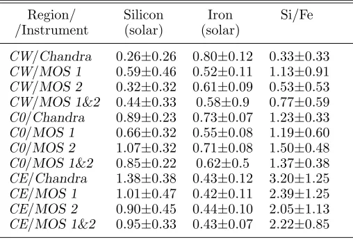
Based on the Si/FeChandramap we selected three
char-acteristic regions for a direct comparison of the chemi-cal enrichment gradient measured withChandra&XMM.
These regions are circular and are denoted by CW (circle west), C0 (circle center), CE (circle east) in Figure 1b. Individual silicon and iron abundances are shown in Ta-ble 2 and their ratios derived from different instruments are plotted in Figure 5b. In Figure 5b we also show the theoretical limits for 100% SN II Fe mass fraction (top horizontal line) and 100% SN Ia Fe mass fraction for four theoretical supernova explosion models that differ in their explosion characteristics (Nomoto et al. 1997a, b). The error weighted average of the SN Ia Fe mass fraction con-tribution for CW is found to be 100+0.00
−0.09% as opposed to
33±22% found for the CE region.
6. discussion
In this work we re-analyzed the Chandra observation
of Abell 576 and determined the spatial distribution of temperatures, individual elemental abundances and radial velocities of the ICM, using the full field of view of the ACIS-S3 and also two new XMM observations covering
similar spatial scales. This allowed us to compare the re-sults obtained with different instruments having different systematic uncertainties. The velocity distribution near the core of the cluster shows a strong velocity gradient, in very good agreement both in magnitude and direction with the velocity gradient found with both SISs onboard
ASCA. The error weighted average (over ACIS-S3, MOS
1 & MOS 2) maximum velocity difference is found to be (5.9±1.6)×103km s−1. The combined set of observations
makes the significance of velocity detection>99.9%
confi-3
There is evidence that both spatial and temporal variations can be larger at later times (DB06).
4
5
dence, when standard (1σ) gain fluctuations are taken into account.
We also found a strong chemical gradient in the intr-acluster gas of this cluster. The distribution of iron and silicon abundances is asymmetric in such a way as to pro-duce a clear separation of the Si/Fe ratio at the cluster’s center. If converted to SN Type enrichment, the results indicate that nearly 67% of the Fe mass has been produced by SN II towards the E and that the Fe mass content in the ICM towards the W and NW direction has been fully pro-duced by SN Ia (<9% produced by SN II). This chemical gradient is very asymmetric, not consistent with the ra-dial chemical gradients found in some other clusters (e.g. Dupke 1998; Dupke & White 2000a,b 2003; Finoguenov et al. 2000; Allen et al. 2001; De Grandi et al. 2004 Baumgartner et al. 2005). The general characteristics of this cluster are consistent with a merging origin as pro-posed by KD04. However, the velocity gradient in A576 suggests a larger line-of-sight component for the merger axis.
The distribution of galaxy velocities in the field of A576 do not show any clear spatial segregation (Rines et al. 2000). However, the distribution of galaxies (from the NED database5) with redshift within r
200 shows at least
two large concentrations between 0.03<z<0.07 (Figure 6a). The first one is centered at z∼0.0387, which is the characteristic cluster redshift. Since the velocity gradi-ent found with Chandra & XMM is very high we
con-sider also the second galaxy clump at z∼0.065. We sepa-rate three galaxy groups based on redshift: a low z group (0.03<z<0.0387), a high z group (0.0387<z<0.05) and a very high z group (0.057<z<0.07). We plot the galax-ies for these three groups in Figures 6b,c. It can be seen from Figure 6b that the distribution of the 97 low z galax-ies (blue) seem more isotropic than that of the 76 high z galaxies (red) , which seems to be more concentrated to-wards the SW of the cluster. The distribution of the 24 very high z galaxies (magenta) is displaced even more to the SW. Figure 6c shows a blow-up of Figure 6b with the velocity centroids of the three redshift groups (shown by “X”s with the corresponding group colors). The velocity centroids are 2′.4 (2′.2) away form the X-ray center for the low (high) z group. The X-ray center is also ∼>1′.3 from the line connecting the centroids of the two groups, This difference is significantly out of the error ellipsoid for the velocity centroid (assuming 6×10⁻⁵and 2′′.5 errors for
redshift & position, respectively (NED)).
It is very difficult to make a direct comparison between the velocity measurements obtained from galaxy veloci-ties and X-ray measurements given the difference of spa-tial scales. In general, the optical results are not inconsis-tent with the X-ray measurements. However, the absolute values between the redshifts of the galaxy concentrations and those obtained from X-ray spectroscopy are discrepant and the results can only be compatible if there is an over-all gain correction upwards. We do not have an external source to calibrate global gain corrections but it is unlikely that the same correction would affect all three different instruments in different epochs. On the other hand, the methodology used here is sensitive to gain dependence on frequency (e.g., Dupke & Bregman 2001b) and this is likely
the reason for this discrepancy given the low temperatures of teh cluster (the redshift fitting process is weighted by the FeL complex). Even though theabsoluteredshift val-ues may be inaccurate, the redshiftdifferencesshould not be affected, since the same methodology was applied to all regions/and observations. So, we will assume that a cor-rection ofδz∼0.015–0.02 should be applied to all measured redshifts when comparing the data in X-ray and optical frequencies.
The orientation of the low–high velocity regions is very similar to that found in X-ray velocity measurements (NE– SW). We also show the centroid of the joint high & very high z group in yellow. The centroid of this group coin-cides with the most significant high velocity region (Figure 2d). The above mentioned results using galaxy velocities can also be interpreted as due to an unusual amount of interlopers (e.g. Wojtak & Loas 2007) and in this section we discuss two scenarios that can explain the observations, i.e., projection of a background cluster and post-core cross-ing line of sight mergcross-ing.
6.1. Projection Scenario
The results presented above can be at least partially interpreted as resulting from a scenario where A576 is, in reality, two clusters closely aligned in the line of sight. The two clusters could be gravitationally unbound or in a pre-merger stage, in which case the velocity gradient would be mostly attributed to the clusters’ Hubble distances. In this scenario the cores of both clusters would have to be near aligned in order to escape easy identification of a sec-ondary peak in surface brightness.
Optical studies of A576 show several peculiarities that can be interpreted either as consequences of a cluster-cluster merging or as due to projection effects. Rines et al. (2000 - hereafter R00) used the kinematics of the infall region (Diaferio and Geller 1997) of Abell 576 to calculate the mass distribution out to several Mpc. Their method does not need the equilibrium assumptions typically used in X-ray mass estimations and relies on the fact that the velocity field around clusters is determined by the local dynamics of the dark matter halo. The amplitude of the characteristic “trumpet shaped” caustics in their velocity
×radius plot is related to the escape velocity around ha-los. From their analysis one can infer that this cluster is passing through a major disturbance for several reasons, among them, (1) a “finger” in phase space with high ve-locities for radii < 2.9 h−701 Mpc (Figure 4 of R00; see also Rines et al. 2003 and Rines & Diaferio 2006), (2) an apparent deficit of galaxies in the NW of the cluster (Fig-ure 6 of R00), (3) a similar geometrical configuration of high-velocity “background” system (centered nearly 8200 km s−1 over the cluster’s redshift) to the geometrical
con-figuration of the cluster (Figures 14 & 6 of R00), (4) an inferred total mass 2.5 times higher than that found from X-ray analysis in the same spatial scale (see also Mohr et al. 1996).
In order to estimate the likelihood that the velocity gra-dient is due to projection effects we looked at the distribu-tion of galaxy clusters from cosmological N-body Hubble volume simulations. For that we use the positions of clus-ters in a 3 Gpc cube at z≈0 selected in the data generated
5
6
in Evrard et al. (2002). The virtual clusters were gener-ated in a flat ΛCDM model, with Ωm and ΩΛ of 0.3 and
0.7, respectively and σ8=0.9. Clusters were found using
an algorithm that identifies halos as spheres, centered on local density maxima, with radii defined by a mean inte-rior isodensity condition (see Appendix A of Evrard et al. 2002 for details).
We searched within 500000 mock clusters those that had a projected core separation within 180 h−1
70 kpc,
cor-responding to 3.5′ at a redshift ∼0.04. To be conserva-tive we searched for a radial distance separation within 2σ above and below the average redshift difference value of (5.9±1.6)×103 km s−1. The results showed 265
sys-tems that satisfied this criteria indicating a probability of 5×10⁻⁴ to find such systems in the nearby universe.
6.2. Merging Scenario
Local mergers are, however, much more frequent. The same above mentioned Monte Carlo strategy applied to angular scales equivalent to the virial radius of a 4 keV cluster, i.e., r200∼0.85√kTkeV h−701Mpc = 1.7h−701 Mpc,
finds 3.9×10⁴in 5
×105clusters, i.e., a probability of 0.078.
This estimate includes pairs of all relative velocities, but a recent analysis of subhalo–host halo velocity differences found for “bullet clusters” type (1E 0657-56 – Markevitch et al. 2002) halos in the Millennium Simulation (Hayashi & White 2006) indicates that large velocity differences are not uncommon. They find that 40% of all host halos would have 1 out of the 10 most massive sub-halos with a velocity as high as that of the “bullet cluster”. From these stud-ies, we roughly estimate that the likelihood of an ongoing merger with sufficiently high relative velocity is at the per-cent level, and thus a few examples in the local population of observed massive clusters should be expected.
The distribution of gas temperature, iron abundance, abundance ratios suggest that the merging axis compo-nent on the plane of the sky would follow a NW-SE direc-tion. The best configuration that explains the magnitude of the velocity gradient is a scenario similar to that of the “bullet” cluster (1E0657-56), i.e., a violent merger of two colder clusters and a (initial) merger axis making∼ 80◦ with the plane of the sky and a small (∼10◦, see below) deviation with respect to the N–S direction6.
A major prediction of the merging scenario is the pres-ence of a hot (>10 keV if we scale from 1E0657-56) com-ponent correspondent to the bow shock layer on the line of sight. In order to test the consistency of this prediction with the current data we extracted spectra from a large el-liptical region surrounding the cluster’s center covering the outer “temperature ring” seen in Figure 2a as dashed lines (but also including the center). We compared two spectral models fitting simultaneously five data sets, XMMMOS
1 & 2 data from the two pointings and ACIS-S3 data. The first one (model 1) was a single temperature WABS APEC. The second (model 2) was a a double temperature
WABS (APEC + APEC)corresponding to the cold and hot components. The cold component temperature was fixed at 3.5 keV, the lowest temperature observed throughout the temperature map. The normalization of the hot com-ponent was fixed at a fraction, fnorm of that of the cold
component. The number of degrees of freedom in the two models is the same given the constrains imposed to the double temperature component. We varied fnormfrom 1% to 99% and recorded the best-fit parameters. The results are shown in Figure 7a, where we plot theχ2 distribution
as a function of fnorm. It can be seen that the lowestχ2is achieved at∼25% with a corresponding high temperature of 11.8 keV<T<21 keV at the 1σlevel. From Figure 7a we can see that model 2 spectral fittings with fnorm∼>12% is better than those using a single temperature component (model 1), which has aχ2 of 1407 and is shown in Figure
7a as a straight line with a best fit temperature of 4.1 keV. For comparison, we estimated the fractional contribu-tion of the hot component using a recently archived 100 ksec Chandra exposure of 1E0657-56 (Observation ID 5356). In Figure 7b we show the raw X-ray image and the rectangular region used to extract a surface brightness profile along the main direction of motion of the “bullet” to estimate the relative emission measure. The size of the rectangular region (∼25′′) corresponds to ∼3′ region in A576. On Figure 7c we show the surface brightness profile along the slice. From right to left the first sur-face brightness enhancement before the “spike” associated with the cool “bullet” is that of the shock region. Then, we see the colder “bullet” followed by extended peak of the disturbed core of the primary cluster. The last com-ponent is a hot tail. We separated the regions in three parts based on the temperature map in Markevitch et al. (2002). The distribution of photon counts for these three components (again from right to left) is approxi-mately 1000 counts (shock region), 14500 counts (the two cold cores) and 3000 counts (hot tail), which would place the fnorm (hot/cold) at ∼ 26% assuming that the bow shock symmetrically covers the two cluster cores. This fraction can be directly compared to that derived using spectral fittings up to the precision of a (weak) function of temperature f(T) (numbercounts ∝P rojectedArea× Surf Brightness∝ density2×f(T)×P rojectedArea ∝
normalizationV AP EC
characteristic size ×f(T)). It is beyond the scope of this paper to carry out detailed modeling of 1E0657-56. Nev-ertheless, we point out that the overall agreement of fnorm with what would be expected from “seeing” the “bullet” cluster along the merging axis is very consistent with a A576 passing through a near line of sight collision.
With the available data we do not have enough photon statistics and energy coverage to disentangle the multiple temperature components in the line of sight, i.e., cold gas from the pre-shocked ICM, a relatively thin bow shock, the projected high density cold cores, and finally the post and pre shocked material at the largest depth. However, we can roughly estimate a few merger parameters with the data at hand. From simple geometrical principles for a line of sight merger started at a time “-tshock”, the perturbation perpendicular to the surface of the Mach cone will prop-agate with the sound speed, so that the cosα= B
cs tshock,
where α is half angle of the cone, cs is the sound speed given by q5kTICM
3µmp ≈10
3 ( TkeV
3.7keV)
(1
2) km s−1, and B the
projected distance from the merging axis to the point where the sonic perturbation is at a time tshock. Since
6
7
the Mach number M = sinα1 , the time when the shock front was effectively initiated is then tshock = c B
s
√
1−M−2
or tshock ≈(0.08±0.015)h−701 Gy ago, assuming B to be
B= 86±16h−701 kpc∼1′.75±0′.5, where 2B∼3′.5 would be the projected distance between the two “hot” regions (NW & E of the central region) in Figure 2a. The dis-tance traveled by the core along the line of sight during this time isL≈(0.45±0.15)h−1
70 Mpc for M=6±1.6, using
the error-weighted average velocity derived fromChandra
&XMMdata.
The point in the past that the two merging clus-ters overcome the Hubble flow, with zero relative ra-dial velocity (half the orbital period), can be given by
r0 = (2πG2) 1 3(M
c t2cross)
1
3 ≈ 5.5 (M
c15 t
2
crossHub)
1 3 Mpc,
whereMc15 andtcrossHubare the total mass normalized by
1015M
⊙andtcrossHubis the core crossing time normalized
by a Hubble time (set to 1.37×10¹⁰yr). From conservation of energy and angular momentum the relative velocity of the sub-systems at a distance “r” from each other is given by (e.g. Ricker and Sarazin 2001)
v ∼p2 G Mc r−
1 2 (
1−rr0
1−(b r0)
2)
1 2 ≈
4160pMc15 r
−12
0.5M pc ( 1−rr0
1−(b r0)
2)
1
2km s−1,
where b is the impact parameter. If we use the dis-tance between the X-ray peak and the midpoint between the two “hot” regions (= 2B) in Figure 2a as the im-pact parameter we obtain b=50±25 h−1
70 kpc. Taking
the total mass derived by Rines et al. (2000), i.e.,
Mc = (0.72±0.07)×1015h−701M⊙, the relative velocity at
r = L, when the merger shock is effectively initiated, is found to be (3.8±0.63)×103km s−1. This is in the lower
end, but consistent, within the errors, with the observed velocity gradient, described in the previous paragraphs.
As pointed by Dupke & Bregman (2002) and Sunyaev et al. (2003) ICM velocity detections can be corroborated by the use of the kinetic S-Z effect (Sunyaev & Zel’dovich 1970, 1972, 1980). Intracluster gas bulk velocities as high as those detected in A576 should generate significantly dif-ferent levels of Comptonization of the cosmic microwave background radiation (CMBR) towards different direction
of the cluster (red-shifted and blue-shifted sides). The to-tal CMBR temperature variation towards the direction of a moving cluster has a thermal and a kinetic component:
(∆T
T )ν = [ kTe mec2
(xe x+ 1
ex−1 −4)− Vr(b)
c ]τ, (1)
where Te & T are respectively the ICM and CMBR temperatures, Vr is the radial velocity, x= kThν and the other parameters have their usual meanings (Sunyaev & Zel’dovich 1970, 1972, 1980). If the gas number density
n(r) follows a king-like profile n(r) = n0(1 + (rrc)2)−
3 2β,
where rc andn0 are respectively the core radius and the
central density, the Thompson optical depth is given as a function of the projected radius “rproj” by τ(rproj) = σTn0rcB(12,32β−12)(1 + (rprojrc )2)−
3 2β+
1
2, whereB(p, q) =
R∞
0 xp−
1(1 +x)p+qdxis the Beta function of p, q. Using β=0.64,rc=240h−501 kpc, andn0=2×10⁻³cm−3(Mohr et
al 1996), τ ∼ 1.3×10⁻³ and from equation (1) we get
(∆T
T )217GHz = 2.6×10−
5, near the optimal frequency to
observe the kinetic effect. This effect could be detected with current (or in development) instruments, such as the BOLOCAM7, ACBAR (Runyan et al. 2003), SuZIE
(Holzapfel et al. 1997) or Planck8.
The low photon statistics limits our ability to fully dis-entangle the 3-D physics of the merging event to make a close comparison to theoretical/numerical models. How-ever, this work suggests that the temperature, abundance and velocity distributions in Abell 576 are consistent with a scenario where the cluster is passing through a line of sight merger similar to that in the “bullet” cluster. If cor-roborated, this could provide a unique template to study supersonic line of sight cluster merger collisions. This work also illustrates the power of elemental abundance gradient distribution in determining the evolutionary stage of clus-ters.
The authors would like to thank Jimmy Irwin, Ed Lloyd-Davies, Maxim Markevitch, Chris Mullis, Kenneth Rines and Ming Sun for useful discussions and suggestions. We also thank the anonymous referee for useful suggestions. We acknowledge support from NASA Grants NAG 5-3247, NNG05GQ11 & GO5-6139X. This research made use of the HEASARCASCA database and NED.
REFERENCES
Allen, S. W., Fabian, A. C., Johnstone, R. M., Arnaud, K. A., & Nulsen, P. E. J. 2001, MNRAS, 322, 589
Anders, E., & Grevesse N. 1989, Geochimica et Cosmochimica Acta, 53, 197
Andersson, K. E., & Madejski, G. M. 2004, ApJ, 607, 190
Arnaud, K. A. 1996, in Astronomical Data Analysis Software and Systems V, ASP Conf. Series volume 101, eds. Jacoby, G., & Barnes, J., p.17
Baumgartner, W. H., Loewenstein, M., Horner, D. J.& Mushotzky, R. F. 2005, ApJ, 620, 680
Beers, T., 1982, ApJ, 257, 23
Benatov, L., Rines, K., Natarajan, P., Kravtsov, A., & Nagai, D, 2006, MNRAS, in Press
Churazov, E., Gilfanov, M., Forman, W., & Jones, C. 1999, ApJ, 520, 105
David, L. P., Slyz, A., Jones, C., Forman, W., Vrtilek, S. D., & Arnaud, K. A. 1993, ApJ, 412, 479
De Grandi, S., Ettori, S., Longhetti, M., & Molendi, S. 2004, ˚a, 419, 7
Diaferio, A., & Geller, M. J 1997, ApJ481, 633 Dupke, R. A., 1998 PhD Thesis. University of Alabama Dupke, R. A., & White, R. E. III 2000a, ApJ, 528, 139 Dupke, R. A., & White, R. E. III 2000b, ApJ, 537, 123 Dupke, R. A., & White. R. E. III 2003, ApJ, 583, L13. Dupke, R. A., & Bregman, J. N. 2001a, ApJ, 547, 705. Dupke, R. A., & Bregman, J. N. 2001b, ApJ, 562, 266. Dupke, R. A., & Bregman, J. N. 2002, ApJ, 575, 634. Dupke, R. A., & Bregman, J. N. 2005, ApJS, 161, 224 (DB05) Dupke, R. A., & Bregman, J. N. 2006, ApJ639, 781 (DB06) Evrard, A. E. 1990, ApJ, 363, 349;
Evrard, A. E., Metzler, C. A., & Navarro, J. F. 1996, ApJ, 469, 494; Finoguenov, A., David, L. P.;& Ponman, T. J. 2000, ApJ, 544,188 Fukazawa, Y., Ohashi, T., Fabian, A. C., Canizares, C. R., Ikebe,
Y., Makishima, K.,
7
http://www.astro.caltech.edu/˜lgg/
8
8
Gibson, B. K., Loewenstein, M. & Mushotzky, R. F. 1997, MNRAS, 290, 623
Grant, C. 2001, ACIS MEMO 195 space.mit.edu/ACIS/ps files/ps195.ps.gz Hayashi, E. & White, S. D. M., 2006, MNRAS, in Press,
astro-ph/0604443
Holzapfel, W. L., Wilbanks, T. M., Ade, P. A. R., Church, S. E., Fischer, M. L., Mauskopf, P. D., Osgood, D. E. & Lange, A. E. 1997, ApJ479, 17
Inogamov, N. A., & Sunyaev, R. A. 2003, Astron. Lett., 29, 791 Katz, N., & White, S. D. M. 1993, ApJ, 412, 455;
Kay, S. T., Thomas, P. A., Jenkins, A., & Pearce, F. R., 2004, MNRAS, 355, 1091
Kempner, J., & David, L. 2004, ApJ, 607, 220 (KD04)
Landau, L, & Lifshitz, E. 1986, Hydrodynamics, in Theoretical Physics vol 6, page 489, Nauka, Moscow.
Liedahl, D. A., Osterheld, A. L., & Goldstein, W. H. 1995, ApJ, 438, L115
Loewenstein, M. & Mushotzky, R. F. 1996, ApJ, 466, 695
Lucey, J. R., Currie, M. J., & Dickens, R. J. 1986a, MNRAS, 221, 453
Lucey, J. R., Currie, M. J., & Dickens, R. J. 1986b, MNRAS, 222, 427
Markevitch, M. et al. 2002, ApJ, 567, 27
Mushotzky, R. F., & Yamashita, K. 1994, PASJ, 46, 55
Mohr, J. J., Geller, M. J., Fabricant, D. G., Wegner, G., Thorstensen, J., & Richstone, D. O. 1996, ApJ, 470, 724
Morrison, R., & McCammon, D. 1983, ApJ, 270, 119
Navarro, J. F., Frenk, C. S., & White, S. D. M. 1995 MNRAS, 275, 720
Nomoto, K., Iwamoto, K., Nakasato, N., Thielemann, F.-K., Brachwitz, F., Tsujimoto, T., Kubo, Y. & Kishimoto, N., 1997a, Nuclear Physics A, Vol. A621, 467c
Nomoto, K., Hashimoto, M., Tsujimoto, T., Thielemann, F.-K., Kishimoto, N., & Kubo, Y. 1997b, Nuclear Physics A, Vol. A616, 79
Ota, N. et al. 2007, PASJ, 59, 351
Pawl, A., Evrard, A. & Dupke, R. 2005, ApJ, 631, 773
Pearce, F. R., Thomas, P. A., & Couchman, H. M. P. 1994, MNRAS, 268,953;
Peres, C. B., Fabian, A. C., Edge, S. W., Johnstone, R. M., & White, D. A. 1998, MNRAS, 298, 416
Rasia, E., Tormen, G., & Moscardini, L., 2004, MNRAS, 351, 237 Rasia, E., Ettori, S., Moscardini, L., Mazzotta, P., Borgani, S., Dolag,
K., Tormen, G., Cheng, L.M., & Diaferio, A. 2006, MNRAS, Submitted, astro-ph/0602434
Ricker, P. M. 1998, ApJ, 496, 670
Ricker, P. M. & Sarazin, C., 2001, ApJ, 561, 621
Rines, K., Geller, M. J., Diaferio, A., Mohr, J. J., & Wegner, G. A. 2000, AJ, 120, 2338
Rines, K., Geller, M. J., Kurtz,M., & Diaferio, A., 2003, AJ, 126, 2152
Rines, K., & Diaferio, 2006, AJ, 132, 1275
Roettiger, K., Burns, J. O., & Loken, C. 1993, ApJ, 407, 53; Roettiger, K., Burns, J. O., & Loken, C. 1996, ApJ, 473, 651 Roettiger, K., Loken, C., & Burns, J. O. 1997, ApJS, 109, 307 Rothenflug, R., Vigroux, L., Mushotzky, R. F., & Holt, S. S., ApJ,
279, 53
Runyan, M. C., Ade, P. A. R., Bhatia, R. S., Bock, J. J., Daub, M. D., Goldstein, J. H., Haynes, C. V., Holzapfel, W. L., Kuo, C. L., Lange, A. E., Leong, J., Lueker, M., Newcomb, M., Peterson, J. B., Reichardt, C., Ruhl, J., Sirbi, G., Torbet, E., Tucker, C., Turner, A. D., & Woolsey, D. 2003, ApJS149, 265
Smith, R. J., Lucey, J. R., Hudson, M. J., Schlegel, D. J. & Davies, R. L. 2000, MNRAS313, 469
Sanders, J. S. & Fabian, A. 2002, MNRAS, 331, 273 Stein, P., Jerjen, H., & Federspiel, M. 1997, A&A, 327, 952 Sunyaev, R. A., & Zel’dovich, Ya. B. 1970, Astrophys. Space Sci., 7,
3
Sunyaev, R. A., & Zel’dovich, Ya. B. 1972, Comments Astrophys. Space Phys., 4, 173
Sunyaev, R. A., & Zeldovich, Ya. B. 1980, MNRAS, 190, 413 Takizawa, M., & Mineshige, S. 1998, ApJ, 499, 82;
Takizawa, M. 1999, ApJ, 520,514 Takizawa, M. 2000, ApJ, 532, 183
Draft version February 1, 2008
Preprint typeset using LATEX style emulateapj v. 14/09/00
FIGURE CAPTIONS
Fig. 1.— (a) RawChandraX-ray image of Abell 576. The X-ray contours shown here are used throughout the work. North is up. The lowest contour is centered at RA=110.3762 deg, Dec=+55.7653 deg. The most external contour show the CCD borders and is limited by 110.5<RA<110.25 from left to right and 55.828<Dec<55.686 from top to bottom. The same contours are applied in Figures 2, 5b and 6a but with the scale slightly smaller. (b) Extraction regions used for spectral fittings for detailed analysis of radial velocities (S
¯OUTH and E¯AST), Si/Fe ratio (CW, C0, CE) analyzed in this work. We also indicate the regions found to have high radial velocities (0◦–100◦) and low radial velocities (170◦–250◦) in a previousASCAanalysis (Dupke & Bregman 2005a).
Fig. 2.— Results from an adaptive smoothing algorithm with a minimum of 5000 counts per extraction circular region and fitted with an absorbed VAPEC spectral model. The gridding method used is a correlation method that calculates a new value for each cell in the regular matrix from the values of the points in the adjoining cells that are included within the search radius. With the minimum count constraints the matrix size was 50×50 cells. We also overlay the X-ray contours shown in Figure 1a on top of the contour plot). North is up. The lowest contour is centered at RA=110.3762 deg, Dec=+55.7653 deg. The units are pixels and 1 pixel=0.5 arcsec. The arrow indicates 1 arcminute. The parameters mapped are (a) Temperature (b) Redshift (c) Smoothed redshift error of each cell used in the adaptive binning (d) Deviation significance, i.e., redshift value found in (b) minus the average for the whole CCD divided by the error of each measurement. The dashed ellipses shown in the Temperature plots indicate approximately the direction of the Mach cone in the scenario of near line of sight merger. The two stars near the center of the redshift map indicate the position of two bright E galaxies near the cluster’s X-ray center, with relative line of sight velocity difference of 900 km/s (Smith et al. 2000). The average redshift error for each cell used in the adaptive binning code is is 0.01. The errors for the cells near the bottom left (SE) regions reach 0.02.
Fig. 3.— (a)Best fit values for temperature, Fe abundance and redshift for the S
¯OUTH and E¯AST regions shown in Figure 1b with different instruments. The left data point for instrument shows the value for S
¯OUTH and the right data point the value for E¯AST. MOS 1& 2 represent the results from simultaneous spectral fittings of the two MOS spectrometers. We also indicate the optically determined redshift for the cluster. (b)TOP - Spectral fittings for regions SOUTH (white) and EAST (red) using Chandra ACIS-S3 data. BOTTOM - A blow-up of the more prominent lines in the FeL and FeK complexes with the continuum subtracted. (c)Same as (b) but for the MOS 1 data. (d)Same as (b) but for the MOS 2 data.
Fig. 4.— (a)Probability of detecting a velocity difference greater than ∆V for S
¯OUTH and E¯AST regions. Solid line is without gain fluctuations. The other lines plots assume a 1σ, 2σ, 3σ, 4σand 5σgain fluctuation (500km s−1
for individual velocity differences). Results are obtained from spectral fittings of 500 simulated spectra for each region forChandraandXMM. (b) Smoothed map of the scatter (standard deviation) of the best fit redshifts over three time cuts (epochs) each one having 9.5 ksec duration. Darker regions indicate lowest scatter and therefore higher gain stability. We also overlay the X-ray contours shown in Figure 1a on top of the contour plot). North is up. The lowest contour is centered at RA=110.3762 deg, Dec=+55.7653 deg. The units are pixels and 1 pixel=0.5 arcsec. The arrow indicates 1 arcminute.
Fig. 5.— (a)Results from an adaptive smoothing algorithm described in Figures 2 for the Si/Fe abundance ratio found withChandra data. We also overlay the X-ray contours shown in Figure 1a on top of the contour plot). North is up.The lowest contour is centered at RA=110.3762 deg, Dec=+55.7653 deg. The units are pixels and 1 pixel=0.5 arcsec. The arrow indicates 1 arcminute. (b) Si/Fe abundance ratio measurements (by number normalized to solar) of Regions CW, C0 and CE usingChandraandXMMMOS 1, 2 and 1& combined. We also shown the theoretical predictions for pure SN II enrichment (top horizontal line) and different models of pure SN Ia enrichment (standard W7 and Delayed Detonation models 1,2 & 3 of Nomoto et al. (1997a, b)).
Fig. 6.— (a) Histogram of galaxy velocities within a projected distance of 1 r200 from the X-ray center. Data is from NASA/IPAC
Extragalactic Database (nedwww.ipac.caltech.edu/). (b) Galaxy positions separated by redshift in the histogram shown in (a). Galaxies with redhifts 0.03<z<0.0387 are denoted by blue circles. Red circles denote galaxies with redshifts 0.0387<z<0.05 and magenta circles correspond to 0.057<z<0.07. X-ray contours are also shown inthe center of the figure in white and the SOUTH and EAST boxy regions are shown in green. The large circle in black corresponds to∼1 r200. (c) Blow-up of Figure 6b. Notation is the same as (b). It is also shown the velocity
centroids for different redshift groups with “X”. Blue corresponds to 0.03<z<0.0387, red to 0.0387<z<0.05, magenta to 0.057<z<0.07 and yellow to 0.0387<z<0.07.
Fig. 7.— (a)χ2 variation of the best-fit doubleAPECmodel to a large elliptical region encompassing the central regions of A576 as a function of the ratio of normalizations of the hot to cold components. Intermediate values of the best-fit high temperatures are shown for normalizations ratios of 10%, 24% (lowestχ2) & 70%. The temperature of the cold component was fixed at 3.5 keV. The fit usesXMMMOS 1 & 2 data from the two off-center pointings and ACIS-S3 data simultaneously. The dotted lines show the results for a single APEC with a best-fit temperature of 4.1 keV, for comparison. The number of degrees of freedom in the two models is the same given the constrains imposed to the double temperature component. (b) ACIS-I image of 1E0657-56 from a deep (100 ksec) observation of the cluster. We also show the rectangular slice used to extract the surface brightness profile. North is up. (c) Surface Brightness profile of the bullet cluster (1E0657-56) along the rectangular slice shown in Figure 7b. The X-axis is shown in arcseconds and the Y-axis in arbitrary surface brightness units.
10
Table 1
Spectral Fittings forSOUTH&EastRegionsa,b
Region/ Temperature Abund Redshift χ2/dof
/Instrument (keV) (Solar)c (10−2)
SOUTH/Chandra 3.75+0.18
−0.18 0.47−+00..0808 3.71+0−0..2460 578/398
SOUTH/MOS 1 4.05+0.20
−0.28 0.60 +0.11
−0.16 3.72 +0.56
−0.52 728/429
SOUTH/MOS 2 3.70+0.32
−0.32 0.71−+00..2616 4.76+0−0..2466 728/429
SOUTH/MOS 1&2 3.95+0.20
−0.20 0.62 +0.13
−0.13 4.18 +0.30
−0.30 728/429
EAST/Chandra 3.89+0.25
−0.25 0.40 +0.09
−0.09 1.11 +0.48
−1.08 341/314
EAST/MOS 1 3.98+0.22
−0.22 0.60−+00..1313 2.40+0−0..5653 541/362
EAST/MOS 2 4.09+0.20
−0.25 0.56 +0.07
−0.12 1.19 +2.73
−0.54 541/362
EAST/MOS 1&2 4.03+0.18
−0.18 0.58−+00..1010 1.87+0−0..5720 541/362 aErrors are 1σconfidence
bFull energy range (0.5 keV–9.5 keV) cPhotospheric
Table 2
Individual Elemental Abundances a
Region/ Silicon Iron Si/Fe
/Instrument (solar) (solar)
CW/Chandra 0.26±0.26 0.80±0.12 0.33±0.33
CW/MOS 1 0.59±0.46 0.52±0.11 1.13±0.91
CW/MOS 2 0.32±0.32 0.61±0.09 0.53±0.53
CW/MOS 1&2 0.44±0.33 0.58±0.9 0.77±0.59
C0/Chandra 0.89±0.23 0.73±0.07 1.23±0.33
C0/MOS 1 0.66±0.32 0.55±0.08 1.19±0.60
C0/MOS 2 1.07±0.32 0.71±0.08 1.50±0.48
C0/MOS 1&2 0.85±0.22 0.62±0.5 1.37±0.38
CE/Chandra 1.38±0.38 0.43±0.12 3.20±1.25
CE/MOS 1 1.01±0.47 0.42±0.11 2.39±1.25
CE/MOS 2 0.90±0.45 0.44±0.10 2.05±1.13
CE/MOS 1&2 0.95±0.33 0.43±0.07 2.22±0.85
[image:10.612.182.436.494.667.2]