R E S E A R C H
Open Access
Smoothing approximation to the lower
order exact penalty function for inequality
constrained optimization
Shujun Lian
1*and Nana Niu
1*Correspondence:
1School of Management Science,
Qufu Normal University, Rizhao, China
Abstract
For inequality constrained optimization problem, we first propose a new smoothing method to the lower order exact penalty function, and then show that an
approximate global solution of the original problem can be obtained by solving a global solution of a smooth lower order exact penalty problem. We propose an algorithm based on the smoothed lower order exact penalty function. The global convergence of the algorithm is proved under some mild conditions. Some numerical experiments show the efficiency of the proposed method.
MSC: 90C30
Keywords: Lower order penalty function; Inequality constrained optimization; Exact penalty function; Smoothing method
1 Introduction
Consider the following inequality constrained optimization problem:
minf0(x)
s.t.fi(x)≤0, i∈I={1, 2, . . . ,m},
(P)
wherefi:Rn→R,i= 0, 1, . . . ,m, are twice continuously differentiable functions.
Through-out this paper, we useX0={x∈Rn|fi(x)≤0,i∈I}to denote the feasible solution set.
This problem is widely applied in transportation, economics, mathematical program-ming, regional science, etc. [1–3], and it has received extensive attention on a related problem, for example, variational inequalities, equilibrium problem, minimizers of convex functions, etc. (see, e.g., [4–15]).
To solve problem (P), the penalty function methods have been introduced in many lit-erature works (see, e.g., [16–24]). Zangwill [16] introduced the classicall1exact penalty
function
F1(x,q) =f0(x) +q
m
i=1
maxfi(x), 0
, (1.1)
whereq> 0 is a penalty parameter, but it is not a smooth function. The corresponding penalty optimization problem is as follows:
min
x∈RnF1(x,q). (P1)
The non-smoothness of the function restricts the application of a gradient-type or Newton-type algorithm to solving problem (P1). In order to avoid this shortcoming, the
smoothing of thel1exact penalty function is proposed in [17,18].
In addition, to overcome the non-smoothness of the function, the following smooth penalty function is proposed:
F2(x,q) =f0(x) +q
m
i=1
maxfi(x), 0 2
. (1.2)
However, the function is non-exact.
Recently, Wuet al.[20] proposed the following low order penalty function:
ϕq,k(x) =f0(x) +q
m
i=1
maxfi(x), 0 k
, k∈(0, 1), (1.3)
and proved that the low order penalty function is exact under mild conditions. But this penalty function is non-smooth, too. Whenk= 1,ϕq,k(x) can be seen as the classicall1
exact penalty function. The least exact penalty parameter corresponding tok∈(0, 1) is much less than that of thel1exact penalty function. This can avoid the defects of too large
parameterρin the algorithm. Only fork=12, the smoothing of the lower order penalty function (1.3) is studied in [20] and [21]. In [24], a smoothing method of the low order penalty function (1.3) is given. We hope to study a new smoothing method for the low order penalty function (1.3) and compare it with the existing methods. With a different segmentation method, we will give a new piecewise smooth function and propose a new method to smooth the lower order penalty function (1.3) withk∈[12, 1) in this paper.
The remainder of this paper is organized as follows. In Sect.2, a new smoothing func-tion is proposed. The error estimates are obtained among the optimal objective funcfunc-tion values of the smoothed penalty problem, the non-smooth penalty problem, and the origi-nal problem. In Sect.3, the corresponding algorithm is proposed to obtain an approximate solution to (P). The global convergence of the algorithm is proved. In Sect.4, some nu-merical experiments are given to illustrate the efficiency of the algorithm. In Sect.5, some conclusions are presented.
2 A smoothing penalty function
For the lower order penalty problem
min
x∈Rnϕq,k(x), (LP)
Assumption 2.1
(1) f0(x)satisfies the coercive condition
lim
x→+∞f0(x) = +∞.
(2) The optimal solution setG((P))is a finite set.
Under Assumption2.1, problem (P) is equivalent to the following problem:
minf0(x)
s.t.fi(x)≤0, i∈I,
x∈X,
(P)
whereXis a box withint(X)=∅.
For anyk∈(0, 1), penalty problem (LP) is equivalent to the following penalty problem:
min
x∈Xϕq,k(x). (LP
)
Now we consider a new smoothing technique to the lower order penalty function (1.3). Letpk(t) = (max{t, 0})k, then
ϕq,k(x) =f0(x) +q
m
i=1
pk
fi(x)
. (2.1)
Define a functionpk,(t) (> 0) by
pk,(t) =
⎧ ⎪ ⎨ ⎪ ⎩
0, ift≤–k,
k
2
–1(t+k)2, if –k<t< 0,
(t+)k+k22k–1–k, ift≥0,
(2.2)
where 1
2≤k< 1. It is easy to see thatpk,(t) is continuously differentiable and
lim
→0+pk,(t) =pk(t).
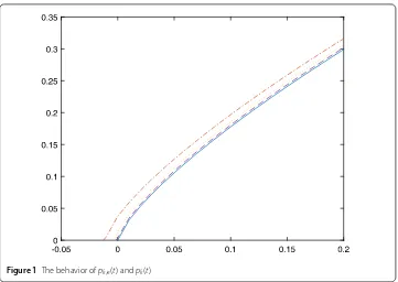
The following figure shows the process of functionpk,(t) approaching functionpk(t).
Figure1shows the behavior ofp3
4,0.01(t) (represented by the dash and dot line),p34,0.001(t)
(represented by the dot line),p3
4,0.0001(t) (represented by the dash line), andp34(t)
(repre-sented by the solid line).
Based on this, we consider the following continuously differentiable penalty function:
ϕq,k,(x) =f0(x) +q
m
i=1
pk,
fi(x)
, (2.3)
wherelimε→0+ϕq,k,(x) =ϕq,k(x).
The corresponding optimization problem toϕq,k,(x) is as follows:
min
Figure 1The behavior ofpk,(t) andpk(t)
For problems (P), (LP), and (SP), we have the following conclusion.
Lemma 2.1 For any x∈X,> 0,and q> 0,it holds that
–k 2
2k–1mq≤ϕq
,k(x) –ϕq,k,(x) <kmq, k∈
1 2, 1
.
Proof For alli∈I, it holds that
pk
fi(x)
–pk,
fi(x)
=
⎧ ⎪ ⎨ ⎪ ⎩
0, iffi(x)≤–k,
–k2–1(f
i(x) +k)2, if –k<fi(x) < 0,
fi(x)k– (fi(x) +)k–k22k–1+k, iffi(x)≥0.
Set
F(t) =tk– (t+)k, t≥0.
Then
F(t) =ktk–1– (t+)k–1.
It is easy to see that functionF(t) is monotonically increasing w.r.t.tdue to thatk∈[12, 1). One has
–k≤fi(x)k–
fi(x) + k≤
0, iffi(x)≥0.
It follows that
–k 2
2k–1≤p
k
fi(x)
–pk,
fi(x)
When –k<f
i(x) < 0, one has
–k 2
2k–1<p
k
fi(x)
–pk,
fi(x)
< 0.
So,
–k 2
2k–1≤p
k
fi(x)
–pk,
fi(x)
<k, ∀i∈I. (2.4)
It follows from (2.1), (2.3), and (2.4) that
–k 2
2k–1mq≤ϕq
,k(x) –ϕq,k,(x) <kmq
by the fact thatq> 0.
Theorem 2.1 For a positive sequence{εj},which converges to0as j→ ∞,assume that xj
is an optimal solution tominx∈Xϕq,k,j(x)for some given q> 0,k∈[
1
2, 1).If x is an
accumu-lating point of sequence{xj},thenx is an optimal solution to¯ min
x∈Xϕq,k(x).
Proof It follows from Lemma2.1that
–k 2
2k–1
j mq≤ϕq,k(x) –ϕq,k,j(x) <
k
jmq, ∀x∈X. (2.5)
Sincexjis a solution tominx∈Xϕq,k,j(x), one has
ϕq,k,j(xj)≤ϕq,k,j(x), ∀x∈X. (2.6)
It follows from (2.5) and (2.6) that
ϕq,k(xj) <ϕq,k,j(xj) +
k jmq
≤ϕq,k,j(x) +
k jmq
≤ϕq,k(x) +kjmq+
k
2
2k–1
j mq.
Lettingj→ ∞yields
ϕq,k(x¯)≤ϕq,k(x).
Thus,xis an optimal solution tominx∈Xϕq,k(x).
Theorem 2.2 Let x∗q,k∈X be an optimal solution of problem(LP),andx¯q,k,∈X be an
optimal solution of problem(SP)for some q> 0,k∈[12, 1),and> 0.Then
–k 2
2k–1mq≤ϕ
q,k
Proof Under the hypothetical conditions, it holds thatϕq,k(xq∗,k)≤ϕq,k(x) andϕq,k,(x¯q,k,)≤
ϕq,k,(x),∀x∈X.
Therefore, by Lemma2.1, one has
–k 2
2k–1mq≤ϕq ,k
x∗q,k–ϕq,k,
x∗q,k≤ϕq,k
x∗q,k–ϕq,k,(x¯q,k,)
and
ϕq,k
x∗q,k–ϕq,k,(x¯q,k,)≤ϕq,k(x¯q,k,) –ϕq,k,(x¯q,k,) <kmq.
This completes the proof.
Corollary 2.1 Suppose that Assumption2.1holds,and for any x∈G((P)),there existsλ∗∈
Rm
+ such that the pair(x∗,λ∗)satisfies the second order sufficient condition(in[20]).Let x∗∈
X be an optimal solution of problem(P)andx¯q,k, ∈X be an optimal solution of problem
(SP)for some q> 0,k∈[12, 1),and> 0.Then there exists q∗> 0such that,for any q>q∗,
–k 2
2k–1mq≤f 0
x∗–ϕq,k,(x¯q,k,) <kmq.
Proof It follows from Corollary 2.3 (in [20]) thatx∗∈Xis an optimal solution of problem (LP). By Theorem2.2, one has
–k 2
2k–1mq≤ϕ
q,k
x∗–ϕq,k,(x¯q,k,) <kmq.
Sincemi=1pk(fi(x∗)) = 0, it holds that
ϕq,k
x∗=f0
x∗+q
m
i=1
pk
fi
x∗=f0
x∗.
This completes the proof.
Definition 1 For> 0, ifx∈Xis such that
fi(x)≤, i= 1, 2, . . . ,m,
thenx∈Xis an-feasible solution of problem (P).
Theorem 2.3 Let x∗q,k∈X be an optimal solution of problem(LP),andx¯q,k,∈X be an
optimal solution of problem(SP)for some q> 0,k∈[12, 1),and> 0.If x∗q,k is afeasible
solution of problem(P),andx¯q,k,is an-feasible solution of problem(P),then
–k 2
2k–1mq≤f 0
x∗q,k–f0(x¯q,k,) <
2kk+k 2
2k–1
Proof By (2.1), (2.3), and Theorem2.2, one has
–k 2
2k–1mq≤ϕ
q,k
x∗q,k–ϕq,k,(x¯q,k,)
=f0
x∗q,k+q
m i=1 pk fi
x∗q,k–
f0(x¯q,k,) +q
m
i=1
pk,
fi(x¯q,k,)
<kmq.
Sincemi=1pk(fi(x∗q,k)) = 0, it holds that
–k 2
2k–1mq+q
m
i=1
pk,
fi(x¯q,k,)
≤f0
x∗q,k–f0(x¯q,k,)
<kmq+q
m
i=1
pk,
fi(x¯q,k,)
. (2.7)
Note that
fi(x¯q,k,)≤, i∈I.
Thus, it follows from (2.2) that
0≤q
m
i=1
pk,
fi(x¯q,k,)
≤
2kk+k 2
2k–1–k
mq. (2.8)
By (2.7) and (2.8), one has
–k 2
2k–1mq≤f 0
x∗q,k–f0(x¯q,k,) <
2kk+k 2
2k–1
mq.
Theorems2.1and2.2show that an optimal solution of (SP) is also an approximate op-timal solution of (LP) when the erroris sufficiently small. By Theorem2.3, an optimal solution of (SP) is an approximately optimal solution of (P) if the optimal solution of (SP) is an-feasible solution of (P).
3 A smoothing method
Based on the discussion in the last section, we can design an algorithm to obtain an ap-proximate optimal solution of (P) by solving (SP).
Algorithm 3.1
Step 1. Takex0,
0> 0,0 <a< 1,q0> 0,b> 1,> 0, andk∈[12, 1), letj= 0and go to
Step 2.
Step 2. Solveminx∈Rnϕq
j,k,j(x)starting atxj. Letxj+1be the optimal solution (xj+1can be obtained by a quasi-Newton method).
Step 3. Letj+1=aj,qj+1=bqj, andj=j+ 1, then go to Step 2.
Remark Since 0 <a< 1 andb> 1, leta2k–1b< 1, asj→+∞, the sequence{
j}is gradually
decreased to 0, the sequence{qj}is gradually increased to +∞and{j2k–1qj}is gradually
Under some mild conditions, the following conclusion shows the global convergence of Algorithm3.1.
Theorem 3.1 Suppose that Assumption2.1holds,and for any∈(0,0],q∈[q0, +∞),
the solution set ofminx∈Rnϕq,k,(x)is nonempty.If{xj+1}is the sequence generated by Algo-rithm3.1satisfying a2k–1b< 1,and the sequence{ϕ
qj,k,j(x
j+1)}is bounded,then
(1) {xj+1}is bounded.
(2) Any limit point of{xj+1}is an optimal solution of(P).
Proof (1) It follows from (2.3) that
ϕqj,k,j
xj+1=f0
xj+1+qj m
i=1
pk,j
fi
xj+1, j= 0, 1, 2, . . . . (3.1)
By hypothesis, there exists some number L such that
L>ϕqj,k,j
xj+1, j= 0, 1, 2, . . . . (3.2)
For the sake of contradiction, suppose that{xj+1}is unbounded. Without loss of generality,
we assume thatxj+1 → ∞asj→ ∞.
By (2.2), (3.1), and (3.2), one has
L>f0
xj+1, j= 0, 1, 2, . . . ,
which results in a contradiction with Assumption2.1(1). (2) Without loss of generality, we assumexj+1→x∗asj→ ∞.
To provex∗ is the optimal solution of (P), it is only needed to show thatx∗∈X0and
f0(x∗)≤f0(x),∀x∈X0.
To show thatx∗∈X0, we outline a proof by contradiction. We presuppose thatx∗∈/X0,
then there existδ0> 0,i0∈I, and the subsetJ⊂Nsuch that
fi0
xj+1≥δ0>j, ∀j∈J,
whereNis the natural number set.
By Step 2, (2.2), and (2.3), for anyx∈X0, one has
f0
xj+1+qj
(δ0+j)k+
k
2
2k–1
j –jk
≤ϕqj,k,j
xj+1 ≤ϕqj,k,j(x) ≤f0(x) +m
k
2
2k–1
j qj.
It follows that
f0
xj+1+qj
(δ0+j)k–jk
≤f0(x) + (m– 1)
k
2
2k–1
j qj, ∀x∈X0,
which contradicts withqj→+∞,j→0, andj2k–1qj→0, asj→ ∞. Then we have that
Next, we show thatf0(x∗)≤f0(x),∀x∈X0.
For this, by Step 2, (2.2), and (2.3), it holds that
f0
xj+1≤ϕ
qj,k,j
xj+1≤ϕ
qj,k,j(x)≤f0(x) +m k
2
2k–1
j qj, ∀x∈X0.
Lettingj→ ∞yields that
f0
x∗≤f0(x).
Therefore, any limit point of{xj+1}is an optimal solution of (P).
4 Numerical examples
In this section, we will do some numerical experiments to show the efficiency of Algo-rithm3.1.
Example4.1 Consider the following optimization problem considered in [18,22,23]:
minf0(x) =x21+x22+ 2x32+x24– 5x1– 5x2– 21x3+ 7x4
s.t.f1(x) = 2x21+x22+x23+ 2x1+x2+x4– 5≤0,
f3(x) =x21+x22+x23+x24+x1–x2+x3–x4– 8≤0,
f3(x) =x21+ 2x22+x23+ 2x24–x1–x4– 10≤0.
For this problem, we letk=34,0= 0.01,a= 0.01,q0= 1,b= 2,= 10–16. With different
starting points, numerical results of Algorithm3.1are shown in Tables1,2, and3. From Tables1,2,3, we know that the obtained approximate optimal solutions are similar, which shows that the numerical result of Algorithm3.1does not depend on the section of the starting points for this example. In [18], the objective function valuef0(x∗) = –44.23040
was obtained in the forth iteration. From the numerical results given in [22], we know that the optimal solution isx∗= (0.1585001, 0.8339736, 2.014753, –0.959688) with the objec-tive function valuef0(x∗) = –44.22965. In [23], the objective function value obtained in
Table 1 Numerical results for Example4.1withx0= (0, 0, 0, 0)
j xj+1 q
j j f1(xj+1) f2(xj+1) f3(xj+1) f0(xj+1)
[image:9.595.115.479.567.604.2]0 (0.185009, 0.804369, 2.015460, –0.952409) 1 0.01 –4.797079 –0.00109 –2.028111 –44.225926 1 (0.169902, 0.835670, 2.008151, –0.965196) 2 0.0001 –9.748052 –9.337847 –1.883271 –44.231252
Table 2 Numerical results for Example4.1withx0= (2, 0, 3.5, 0)
j xj+1 q
j j f1(xj+1) f2(xj+1) f3(xj+1) f0(xj+1)
0 (0.169693, 0.835634, 2.008291, –0.965082) 1 0.01 –9.502428 –8.676884 –1.883244 –44.231403
Table 3 Numerical results for Example4.1withx0= (2, 2, 2, 0.5)
j xj+1 q
j j f1(xj+1) f2(xj+1) f3(xj+1) f0(xj+1)
[image:9.595.114.478.639.667.2]Table 4 Numerical results for Example4.2withk=34
j xj+1 q
j j f1(xj+1) f2(xj+1) f0(xj+1)
0 (3.4217, 2.7082) 2 0.001 4.1300 –0.0053 –15.2492
[image:10.595.118.479.174.212.2]1 (0.8022, 1.1978) 20 0.000001 0.0000 –0.4066 –7.1999
Table 5 Numerical results for Example4.2withk=35
j xj+1 q
j j f1(xj+1) f2(xj+1) f0(xj+1)
0 (4.0607, 3.0227) 2 0.001 5.0834 –0.0153 –16.0434
1 (0.8027, 1.1971) 20 0.000001 –0.0003 –0.4086 –7.1992
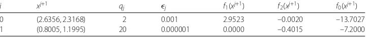
Table 6 Numerical results for Example4.2withk=89
j xj+1 qj j f1(xj+1) f2(xj+1) f0(xj+1)
0 (2.6356, 2.3168) 2 0.001 2.9523 –0.0020 –13.7027
1 (0.8005, 1.1995) 20 0.000001 0.0000 –0.4015 –7.2000
the 25th iteration isf0(x∗) = –44. Hence, the numerical results obtained by Algorithm3.1
are better than the numerical results given in [18,22,23] for this example.
Example4.2 Consider the following problem considered in [17]:
minf0(x) = –2x1– 6x2+x21– 2x1x2+ 2x22
s.t.f1(x) =x1+x2– 2≤0,
f2(x) = –x1+ 2x2– 2≤0,
x1,x2≥0.
For this problem, we letx0= (0, 0),
0= 0.001,a= 0.001,q0= 2,b= 10,= 10–16. With
differentk, numerical results of Algorithm3.1are shown in Tables4,5, and6.
From Tables4,5, 6, we can see that almost the same approximate optimal solutions are obtained for differentkin this example. The objective function value is similar to the objective function valuef0(x∗) = –7.2000 withx∗= (0.8000, 1.2000) obtained in the forth
iteration in [17].
Example4.3 Consider the following problem considered in [24] and [25] (Test Problem 6 in Sect. 4.6):
minf0(x) = –x1–x2
s.t.f1(x) =x2– 2x14+ 8x31– 8x21– 2≤0,
f2(x) =x2– 4x41+ 32x31– 88x21+ 96x1– 36≤0,
0≤x1≤3, 0≤x2≤4.
For this problem, we setk=23,x0= (0, 0),
0= 0.01,a= 0.01,q0= 5,b= 2,= 10–16. The
numerical results of Algorithm3.1are shown in Table7. We setk=89, x0= (1.0, 1.5),
0= 0.1,a= 0.1,q0= 5,b= 3, = 10–16. The numerical
[image:10.595.118.480.248.285.2]Table 7 Numerical results for Example4.3withx0= (0, 0)
j xj+1 q
j j f1(xj+1) f2(xj+1) f0(xj+1)
0 (2.329795, 3.133729) 5 10–2 –0.047009 –0.043471 –5.463524
1 (2.329238, 3.173320) 10 10–4 –0.002868 –0.006501 –5.502557
2 (2.329452, 3.177637) 20 10–6 –0.000302 –0.001176 –5.507089
[image:11.595.117.479.193.269.2]3 (2.329626, 3.177558) 40 10–8 –0.001802 –0.000436 –5.507185
Table 8 Numerical results for Example4.3withx0= (1.0, 1.5)
j xj+1 q
j j f1(xj+1) f2(xj+1) f0(xj+1)
0 (2.330261, 3.061875) 5 10–1 –0.1226776 –0.1131323 –5.392137
1 (2.329664, 3.161611) 15 10–2 –0.018055 –0.016207 –5.491275
2 (2.329639, 3.171941) 45 10–3 –0.007524 –0.005993 –5.501580
3 (2.329560, 3.177804) 135 10–4 –0.001013 –0.000503 –5.507363
4 (2.329593, 3.177793) 405 10–5 –0.001297 –0.000357 –5.507386
5 (2.329622, 3.177781) 1215 10–6 –0.001544 –0.000234 –5.507403
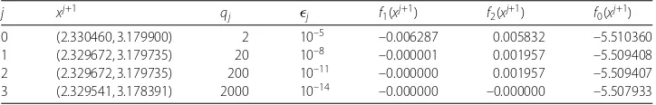
Table 9 Numerical results for Example4.3withx0= (2, 0.5)
j xj+1 qj j f1(xj+1) f2(xj+1) f0(xj+1)
0 (2.330460, 3.179900) 2 10–5 –0.006287 0.005832 –5.510360
1 (2.329672, 3.179735) 20 10–8 –0.000001 0.001957 –5.509408
2 (2.329672, 3.179735) 200 10–11 –0.000000 0.001957 –5.509407
3 (2.329541, 3.178391) 2000 10–14 –0.000000 –0.000000 –5.507933
We setk=34,x0= (2, 0.5),
0= 0.00001,a= 0.001,q0= 2,b= 10,= 10–16. The numerical
results of Algorithm3.1are shown in Table9.
In [24], with three different starting points, similar numerical results are given with
k=23. The optimal solution (2.329517, 3.178421) is given with the objective function value –5.507938. In [25], the optimal solution (2.3295, 3.1783) is given with the objective func-tion value –5.5079. The numerical results of Example 4.3are similar to the numerical results of [24] and [25] in this example.
From Tables7,8,9, we can see that we need to adjust the parametersq0,0,a,bto get
the better numerical results with differentkandx0. Usually,0may be 0.5, 0.1, 0.01, 0.001,
or smaller digits, anda= 0.5, 0.1, 0.01, or 0.001.q0may be 1, 2, 3, 5, 10, 100, or larger digits,
andb= 2, 3, 5, 10, or 100.
5 Concluding remarks
In this paper, we proposed a method to smooth the lower order exact penalty function withk∈[12, 1) for inequality constrained optimization. Furthermore, we proved that the algorithm based on the smoothed penalty functions is globally convergent under mild conditions. The given numerical experiments show that the algorithm is effective.
Funding
This work was supported by the National Natural Science Foundation of China (71371107 and 61373027) and the Natural Science Foundation of Shandong Province (ZR2016AM10)
Competing interests
The authors declare that they have no competing interests.
Authors’ contributions
[image:11.595.117.479.307.365.2]Publisher’s Note
Springer Nature remains neutral with regard to jurisdictional claims in published maps and institutional affiliations.
Received: 11 March 2018 Accepted: 5 June 2018 References
1. Wang, C.W., Wang, Y.J.: A superlinearly convergent projection method for constrained systems of nonlinear equations. J. Glob. Optim.40, 283–296 (2009)
2. Qi, L.Q., Wang, F., Wang, Y.J.: Z-eigenvalue methods for a global polynomial optimization problem. Math. Program.
118, 301–316 (2009)
3. Qi, L.Q., Tong, X.J., Wang, Y.J.: Computing power system parameters to maximize the small signal stability margin based on min-max models. Optim. Eng.10, 465–476 (2009)
4. Chen, H.B., Wang, Y.J.: A family of higher-order convergent iterative methods for computing the Moore–Penrose inverse. Appl. Math. Comput.218, 4012–4016 (2011)
5. Wang, G., Che, H.T., Chen, H.B.: Feasibility-solvability theorems for generalized vector equilibrium problem in reflexive Banach spaces. Fixed Point Theory Appl.2012, Article ID 38 (2012)
6. Wang, G., Yang, X.Q., Cheng, T.C.E.: Generalized Levitin–Polyak well-posedness for generalized semi-infinite programs. Numer. Funct. Anal. Optim.34, 695–711 (2013)
7. Wang, Y.J., Qi, L.Q., Luo, S.L., Xu, Y.: An alternative steepest direction method for optimization in evaluating geometric discord. Pac. J. Optim.10, 137–149 (2014)
8. Wang, Y.J., Caccetta, L., Zhou, G.L.: Convergence analysis of a block improvement method for polynomial optimization over unit spheres. Numer. Linear Algebra Appl.22, 1059–1076 (2015)
9. Wang, Y.J., Liu, W.Q., Caccetta, L., Zhou, G.: Parameter selection for nonnegativel1matrix/tensor sparse decomposition. Oper. Res. Lett.43, 423–426 (2015)
10. Sun, M., Wang, Y.J., Liu, J.: Generalized Peaceman–Rachford splitting method for multi-block separable convex programming with applications to robust PCA. Calcolo54, 77–94 (2017)
11. Sun, H.C., Sun, M., Wang, Y.J.: Proximal ADMM with larger step size for two-block separable convex programming and its application to the correlation matrices calibrating problems. J. Nonlinear Sci. Appl.10(9), 5038–5051 (2017) 12. Konnov, I.V.: The method of pairwise variations with tolerances for linearly constrained optimization problems.
J. Nonlinear Var. Anal.1, 25–41 (2017)
13. Qin, X., Yao, J.C.: Projection splitting algorithms for nonself operators. J. Nonlinear Convex Anal.18, 925–935 (2007) 14. Luu, D.V., Mai, T.T.: Optimality conditions for Henig efficient and superefficient solutions of vector equilibrium
problems. J. Nonlinear Funct. Anal.2018, Article ID 18 (2018)
15. Chieu, N.H., Lee, G.M., Yen, N.D.: Second-order subdifferentials and optimality conditions for C1-smooth optimization problems. Appl. Anal. Optim.1, 461–476 (2017)
16. Zangwill, W.I.: Nonlinear programming via penalty functions. Manag. Sci.13(5), 334–358 (1967)
17. Wu, Z.Y., Lee, H.W.J., Bai, F.S., Zhang, L.S., Yang, X.M.: Quadratic smoothing approximation tol1exact penalty function in global optimization. J. Ind. Manag. Optim.1, 533–547 (2005)
18. Lian, S.J.: Smoothing approximation tol1exact penalty function for inequality constrained optimization. Appl. Math. Comput.219(6), 3113–3121 (2012)
19. Lian, S.J., Zhang, L.S.: A simple smooth exact penalty function for smooth optimization problem. J. Syst. Sci. Complex.
25(5), 521–528 (2012)
20. Wu, Z.Y., Bai, F.S., Yang, X.Q., Zhang, L.S.: An exact lower order penalty function and its smoothing in nonlinear programming. Optimization53, 51–68 (2004)
21. Meng, Z.Q., Dang, C.Y., Yang, X.Q.: On the smoothing of the squareroot exact penalty function for inequality constrained optimization. Comput. Optim. Appl.35, 375–398 (2006)
22. Lian, S.J., Han, J.L.: Smoothing approximation to the square-order exact penalty functions for constrained optimization. J. Appl. Math.2013, Article ID 568316 (2013)
23. Lasserre, J.B.: A globally convergent algorithm for exact penalty functions. Eur. J. Oper. Res.7, 389–395 (1981) 24. Lian, S.J., Duan, Y.Q.: Smoothing of the lower-order exact penalty function for inequality constrained optimization.
J. Inequal. Appl.2016, Article ID 185 (2016).https://doi.org/10.1186/s13660-016-1126-9