An integrated approach to the development of continuous simulations

Sock-Em. Plan. Sci.. Vol. 12. pp. 313-327

0 Pergamon Press Ltd., 1978. Printed in Great Britain

AN INTEGRATED APPROACH TO THE DEVELOPMENT

OF CONTINUOUS SIMULATIONS

JAMES R. BURNS

Department of Systems, Texas Tech University, Lubbock, TX 79409, U.S.A.

and

ONUR ULGEN

Department of Industrial and Systems Engineering, University of Michigan-Dearborn, Dearborn, MI 48128, U.S.A.

(Received 1 September 1977; in revised fotm 18 April 1978)

Abstract-An integrated approach to the development of Forrester-style simulation models is described. The approach incorporates the concept of an interaction matrix to assist in the development of causal loop diagrams and Dynamo flow diagrams. The interaction matrix is derived from the fundamental notions of system dynamics. Premised upon the presumption that a computer-aided procedure for model formulation can expedite, systematize, and operationalize the model formulation process, the integrated approach utilizes the interaction matrix as a data structure within the computer. An algorithm designed to interface with a remote terminal (such as a CRT display) determines the interaction matrix by interrogating a user until sufficient information about the problem of interest has been obtained. This algorithm is also described in the paper. The interrogations both motivate and facilitate the determination of quantities to be included as well as couplings between the quantities. When a quantity or coupling is designated by a user, the algorithm “knows” its identity at the time of user origination. Both algorithm and matrix are illustrated through recourse to a text-book example and the paper concludes with a summarizing discussion of the possible contribution of such an approach.

INTRODUCTION

As governmental and industrial institutions find them- selves embedded in problems which are increased in complexity and intensity, the need for more powerful techniques directed toward coping with these problems becomes ever more manifest. Simulation modeling is well established as a tool appropriate for the study and resolution of these problems. Even so, recent studies[l, 21 show that models often fall short of achiev- ing their intended purposes. In a recent study funded by the National Science Foundation some 230. project directors responded to a mail survey intended to deter- mine the uses and characteristics of currently extant models. It was determined that:

(1) “Not withstanding the great degree of policy in- tent, actual policy application appears to have the highest shortfall of use” ([ 11, p. 4).

(2) “The primary cause of low policy utilization rates for models probably is attributable to the “distance” between model builders and potential-policy makers

([ll, P.

This study furthermore stipulates that “at least one-third and perhaps as many as two-thirds of the models failed to achieve their avowed purposes in the form of direct application to policy problems”. One is inclined to ask what can be done to improve the impact which models should be having upon actual policy application.

The study mentioned above was not intentioned as an assessment of the efficacy of current modeling methodology. However, from the statements above, it is clear that modeling methodologists should consider how changes in conventional methodology might mitigate the shortcomings alluded to. It is the thesis of this paper that, through computer-assistance, it would be possible to lessen the “distance” between model builders, analysts and policy makers. Such an approach could

conceivably allow for policy maker participation in the model formulation exercise, could expedite the process of model development, making it less expensive while shortening model development time. Such shortened response periods might enable users to employ sophisti- cated models in crisis management situations.

The formulation of algorithms for this purpose forces a rigorous statement of the principles underlying the methodology. Specifically, the rules of system dynamics[6,7] are employed in the procedure to be discussed. Such algorithms would, when used, neces- sitate a systematic consideration on the user’s part of the important aspects of the model structure. The approach would divide the labor of modeling into human and computer portions where the part not requiring human judgment is automated. The computer aids would also force the modeler to structure his model in a fashion consistent with the requirements of system dynamics methodology. Additionally, computer aids would allow for policy-maker participation in the model formulation process thereby increasing his understanding of model assumptions and structure while lessening model development costs. The policy-maker participatory methodologies of Kane [ 131 and Warfield [ 181 have already demonstrated their usefulness. If applied to simulation model-building, the approach might alleviate conventional problems of tedium, credibility and validity.

314 J. R. BURNS and 0. UWEN The procedure outlined in this paper will start not from

the causal loop diagram but from scratch. Moreover, the approach taken herein is called the ~n~egffffe~ approach because quantities, couplings, and their classifications are determined simultaneously. This is in contradistinc- tion to the approach taken in [3,4] which utilizes the separation conjecture of Warfield ([ 181, p. 63) first to list quantities, then to determine the couplings between the quantities and finally to classify couplings and quantities. (The separation principle avows that “greater intellectual productivity can be achieved by.. .conscious separation of mental activity into distinct idea actions. . .“)

In addition to the integrated concept, the approach utilizes the notion of sector. A sector is a sub-structure of a causal loop diagram which contains all the structure directly associated with a material flow. Each sector contains one and only one materiai flow as shall be explained in later sections of the paper. The relationship of the notion of sector to the approach taken in [4] has been explored in [19]. The discussion in this paper concretizes and extends earlier results discussed in both [4] and [ 191.

Finally, in the approach to be presented, the possibility for computer-assistance in the formulation of system dynamics models is demonstrated. Structural informa- tion tradition~ly exhibited by means of the causal loop diagram (CLD) or the Dynamo flow diagram (DFD) can be stored in the computer’s memory by means of an “interaction matrix”. Other similar model-building methodologies-see Kanefl31, Wakeland[l7], and Molf et al.[iS]--expediciously utilize the notion of an inter- action matrix. The use of interaction matrices in connec- tion with system dynamics models was explored in [19]. Such matrices specify the interactions for all pairs (qi, qj) defined on the Cartesian product Q x Q, where Q is a set of quantities.

In the next section the set-theoretical notions of system dynamics developed in [3,4] will be reviewed in relation to their implications for the interaction matrix formaily developed in [19]. In the section following, an algorithm for the integrated approach is described. The steps which comprise the algorithm are then illustrated through recourse to a textbook example. The specific queries which the ~gorithm would ask are indicated in the “example” section. The example is shown to faith- fully conform to the format of the interaction matrix. In the last section, concluding assessments as to the relative contribution of the approach are given.

ASSERTIONS OF SYSTEM DYNAMICS

In previous papers[4,19], the assertions of system dynamics have been reformulated using set and graph theory. In this section, those set-theoretic assertions will be restated in such a fashion as to allow for a non- rigorous heuristic rationalization of the interaction matrix. The interaction matrix has already been formally and rigorously derived [ 191.

The couplings adjacent to or associated with a quantity qi are designated by means of the sets A,(q)), EC(qi), in which AC(e) denotes those couplings directed-toward qj (in the causal loop diagram) and EC(qj) denotes those couplings directed away-from qj. From systems dynamics[6,7], couplings represent either a transfer of substance (a flow, denoted fl or a transfer of in- formation (denoted I). Definitions for these two coupling types appear later in this section.

Similar conventions are used for the quantities which are coupled to the quantity under consideration qfi E,(qi) denotes those quantities in Q (the quantity set) which are coupled to qj by means of couplings directed away from qi (in the causal loop diagram) and A,(qj)

denotes those quantities which are coupled to qi by means of couplings directed toward qi.

Set and logical symbols are also employed as follows. The notation A,(qi! C I, for example, denotes the pro- position that A,(qi) IS a subset of the set Z of information couplings. When this proposition is simultaneous with the proposition Ec(qjf C Z (denoting that the outward directed couplings are information couplings) then the compound proposition is written A,(qj) C Z A E(qi) C I. Such pro- positions are used to define each of the five basic quantity types in system dynamics. These are stated below, in which X denotes the set of states, R denotes the set of rates, V

denotes the set of auxiliaries, PU denotes the set of parameters and inputs, and Y denotes the set of outputs.

States. A quantity is a state (qf E X) if

or if

&(qi) f F A E=(qi) C Z (I)

Aa C R A &(qf) C YRY (2)

This definition asserts that (in the causal loop diagram) flow couplings are directed toward states and i~ormation couplings are directed away from states. In addition, states are affected only by rates, and states may affect auxiliaries, outputs, or other rates.

Rates. A quantity qi is a rate (qi E R) if

or if

A,(qi) C Z A Z%(qi) C F (3)

A&i) c PUVX A E&i) G X (4) This definition requires that (in the causal loop diagram) information couplings are directed toward rates and flow couplings are generally directed away from rates. Fu~hermore, rates may be affected by parameters, inputs, auxiliaries, or states, and rates may affect states. The remaining definitions are given without justification.

Auxiliaries. A quantity is an auxiliary (qi E V) if A.z(qi) c Z A ZC(qi) C Z

or if

A,(qf) C PUVX A Z&(qif c RVY.

Parameters and inputs. A quantity is a parameter or

an input (qi E PU) if

A,(qi)= 4 A -C(qi) C Z

or if

A&)=# A E&i) c RVY.

Outputs. A quantity is an output (qi E Y) if

An integrated approach to the development of continuous simulations 315

or if

A,(qi) Z PUVX A &(qi)=d.

Since each member of a particular quantity subset, such as X, V or R, must by its de~nition, possess certain properties, all members of the quantity subset must possess the properties. Consequently, the following postulates represent restatements of the definitions given above.

Properties of the set of states X:

A,(X) C F A E,(X) c I,

A,(X) c R A E,(X) c VRY.

Properties of the set of rates R:

0)

(2)

A,(R) 5 I A E(R) c F, A,(R) c PLJVX n E,(R) c X.

Properties of the set of auxiharies V:

(3) (4)

into sector quantities Qi, and between-sector quantities f.&. A sector will refer to a sub-structure (consisting of quantities and couplings) that can be associated with one and only one flow. Thus every flow defines a separate sector. All states and rates which either accumulate or control the flow are included within the sector. Auxili- aries are included within a sector only if they affect and are affected by other quantities known to be contained within a particular sector. Parameters and inputs are included only if they directly affect other quantities in the sector, while outputs are included within the sector if they are functions exclusively of quantities within that sector. Quantities which appear at the interface between two or more sectors are denoted by Qb = { Vbr PU,,, Y,}. By the definition of sector, between-sector quantities cannot include those quantities which control or ac- cumulate flows, i.e. rates and states. All flows must occur within a sector and whenever a flow is observed, a sector must be defined for it. We define Qb as follows:

between-sector quantities Q,,. Qb includes those quantities left over from the set subtraction Q- iG, Qi for a system of n sectors.

A,(V) c I A E,(V) c I. (5)

A,(V) f PUVX A E*(V) c RVY. 6)

Properties of the set of parameters and inputs PU:

THE lNTERACTtON MATRIX

A,(PU) = 4 t, E,(PlJ) C I,

A,(PU) = 4 A E,(Pu) E; RVY.

Properties of the set of outputs Y:

(71

(8)

A,(Y) C 1 A E,(Y)= (b, (9)

A,(Y) c PUVX A E,(Y)=& (10)

In the postulates above, A,(X) denotes the entire set of couplings directed toward al1 states, while E,(X) denotes the entire set of couplings directed away from a11 states. The claim of postulate (1) is that couplings direc- ted toward states are flow couplings, whereas couplings directed away from states are information couplings. This claim is substantiated by the first part of the definition for states. Since by definition each state possesses this property, all states possess the property. All of these definitions and properties are premised upon the consistency supposition [4]. A similar justification for the remaining nine properties is omitted here. See Ref.[l9] for a thorough, formal derivation of these postulates.

The following definitions are given for flow and in- formation couplings.

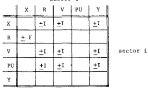
With these brief concepts it is possible to introduce formaliy the interaction matrix. For simplicity the inter- action matrix prescribing a two-sector system is consi- dered, as shown in Fig. 1. below, Thus for a two-sector system, the interaction matrix can be partitioned into two sector matrices and two interconnection matrices. The interconnection matrices specify interactions between sectors, while the sector matrix specifies the interactions within a particular sector. Specifically, the i + j inter- connection matrix specifies the interactions directed from sector i toward sector j and conversely for the j-i interconnection matrix. The sector and intercon- nection matrices are each discussed in what follows.

Tire sector matrix. The sector matrix is indexed by the sets X, R, V, PU and Y as shown in Fig. 2 below. The possible interactions in the sector matrix are indicated by a “2 I” or “?F”, where “t I” denotes possible in- formation couplings, while “2 F” denotes possible flow couplings between members of the associated sets.

Flow couplings. Any coupling Cij = (qi, qi) whose qi is a rate or whose qj is a state, is a flow coupling; mathe- matically, this is written

Sector i sector j

;;I

Fig. I. Interaction matrix for a two-sector system (no quantities between sectors are considered).

sectme i

qi E R v qj E X * cii E F.

I~fo~utio~ coupfi~g~. Any coupling c;i = (qis 41) whose qz is not a rate and whose qi is not a state is an

information coupling; thus sector i

q,EPUVXAqjE VRY$c,EI.

316 J. R. BURNS and 0. ULGEN

Submatrices that are blank represent situations in which interactions cannot occur without producing a violation of the basic rules of system dynamics. For example, no entries can be placed in the (X,X) or (X,PU) sub- matrices because, according to the rules of system dynamics it is impossible for states to affect states directly or to affect parameters and inputs. The matrix can also be rationalized through a consideration of the set theoretic properties for rates, states, etc., provided earlier. By means of properties (1) and (2) above it is clear that states X may affect only rates R, auxiliaries V,

and outputs Y, and each by means of information trans- fers. This is depicted in the first row of the sector matrix shown in Fig. 2. Properties (1) and (2) also suggest that it is possible for states X to be affected only by rates R,

such affect being induced by means of flow couplings. This is depicted in the first column of the sector matrix. A similar consideration of the right-hand portions of properties (3-10) for the remaining subset types justifies the remaining 4 rows of the sector matrix depicted above. An inspection of the columns reveals that the requirements of the left-hand sides of the properties are also satisfied.

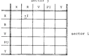
The interconnection matrix. The interconnection

matrix relating sector i to sector j is shown in Fig. 3 below. Clearly, many submatrices do not contain any interactions. By virtue of the definition of “sector”, it is virtually impossible for quantities in V, PU or Y of sector i to affect or be affected by quantities in V, PU or Y of sector j. Thus the submatrix indexed by V, PU and Y along both the row and column is entirely blank. It is also impossible for rates R to affect any quantities in another sector without violating the definition of a sector or property (4) above. However, states X may directly influence rates R in another sector. States may not influence auxiliaries or outputs within another sector as those quantities must possess affector and effector subsets entirely contained within their respective sector(s). Thus the interconnection matrix allows only for interactions directed from states in sector i to rates in sector j.

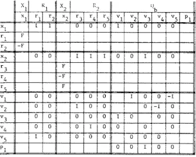
It is possible for some quantities to be incapable (by our conventions) of being associated with any one sec- tor. Such quantities appear at the interface between two or more sectors and include auxiliaries Vb, parameters and inputs PU,, and outputs Yb. These between-sector quantities Qb must also be included in the interaction matrix in situations where they are required. The inter- action matrix for two sectors with between-sector quan- tities included appears in Fig. 4.

Matrices labeled d in the interaction matrix depicted in Fig. 4 are simple sector matrices previously described, while matrices labeled %? will be recognized as inter- connection matrices. Matrix 58 is the matrix of in- formation couplings directed from sector i directly (i.e.

tar ,

sector i

Fig. 3. Possible interactions in the interconnection matrix.

Fig. 4. Detailed interaction matrix for two-sector system (between sector quantities included).

there are no between-sector quantities) toward sector j, while matrix 3)’ is the matrix of information couplings directed from sector j directly toward sector i. Matrix 8 is the matrix exhibiting the possible interactions amongst the between-sector quantities. Matrices labeled % exhibit where and how quantities within sectors i and j can affect or influence between-sector quantities, while matrices labeled 9 exhibit where and how between-sector quantities can influence quantities within sectors i and j. Matrices V and 9 could also be thought of as inter- connection matrices, but to avoid possible confusion with matrices 3, these matrices shall be referred to as interface matrices. Note that the only matrices in which flow couplings can occur are in the sector matrices labeled d-all remaining matrices contain exclusively information couplings.

If the interaction matrix were used in a computer- assisted model formulation exercise, an interrogation would be performed by the computer for each of the entries in which a possible interaction could take place. Using the interaction matrix as its data structure, the computer would insist upon a comprehensive considera- tion of all feasible interactions that are consistent with the rules of system dynamics. A thorough justification of the format of the interaction matrix is found elsewhere[l9].

TiiE ALGORITHM

The algorithm embodying the integrated approach is broken into phases which are illustrated and described by what follows. Employed in an interactive time-shar- ing, computational mode, the algorithm interrogates a user or panel of users until sufficient i~ormation about the issue of interest has been obtained. The sequence of interrogations are intended to both motivate and facili- tate the development of the model structure. The responses resulting from the sequence of interrogations would be stored in the data structure prescribed by the interaction matrix. The algorithm assumes that its users can identify the important quantities and interactions in the system.

An integrated approach to the development of continuous simulations 317

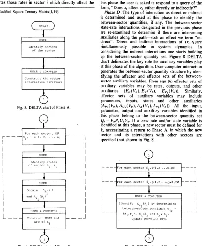
Phase A. Model builders identify the sectors (subsys- set of states in sector i, and conversely for Axi( At tems) of the system and consider the agregate inter- the last step of Fig. 6, in constructing the MSTM of the actions among the sectors. Later phases may require the system sectors Si, the user identifies the sign of inter- introduction and/or elimination of one or more sectors. A actions Cii as positive or negative between the within- comparison of the initial intuitive sector model with the sector states and rates by responding to the queries final model will point out the directions taken with asked by the computer. The specific queries posed by respect to the assumptions, level of detail, and the algorithm are derived from the information supplied components of the system. A DELTA chart of Phase A by the user during previous steps and by the possible

is depicted in Fig. 5. interactions as dictated by the interaction matrix.

Phase B. Since the states of a system are easiest to identify, especially after the sectors of the same are specified, this phase considers first the state variables of each sector. Then the rates that control each level vari- able are identified and for each sector a state-rate inter- action MSTMt and DFD is constructed, in accordance with the DELTA chart in Fig. 6 below, where ARi(Xi) denotes those rates in sector i which directly affect the

tModified Square Ternary Matrix[4,191.

Phase C. In this phase the algorithm asks queries to obtain the interaction structure between the states of one sector and the rates of other sectors. The type of interaction, direct or indirect, is not considered at this stage. The DELTA chart of this phase, depicted in Fig. 7, uses the notation Axi to denote states in sector j which affect, directly or indirectly, rates in sector i. In this phase the user is asked to respond to a query of the form, “Does xl affect rk either directly or indirectly?”

Phase D. The type of interaction as direct or indirect is determined and used at this phase to identify the between-sector quantities, if any. The between-sector state-rate interactions designated in the previous phase are re-examined to determine if there are intervening auxiliaries along the path-such an effect we term “in- direct”. Direct and indirect interactions of (x,, rk)are simultaneously possible in system dynamics. In considering the indirect interactions one starts building up the between-sector quantity set. Figure 8 DELTA chart delineates the key role the auxiliary variables play at this phase of the algorithm. User-computer interaction generates the between-sector quantity structure by iden- tifying the affector and effector sets of the between- sector auxiliary variables. From eqn (6) effector sets of auxiliary variables may be rates, outputs, and other auxiliaries (ER( V,), Eu( V,), EV,,( V,)). Similarly, affector sets of auxiliary variables may include parameters, inputs, states and other auxiliaries (AP~(V~),AU~(V~).AX(V~),AV~(V~)). All the input, parameter, output and auxiliary variables identified in this phase belong to the between-sector quantity set Qb = v&,&Yb. If a new rate and/or state variable is identified at this phase, a new sector must be defined for it, necessitating a return to Phase A, in which the new sector and its interactions with other sectors are specified (not shown in Fig. 8).

start

I

USER

Identify sectors

of the system

Fig. 5. DELTA chart of Phase A.

1

L__

Fig. 6. DELTA chart of Phase B.

For each sector Si.i=l,2,...n.00

by determining

6

318 .J. R. BURNS and 0. ULGEN

r---

I

L__

-,+,--- For path betwren-sector ronplinq

USER & COMPUTER

Identify ZRCVb), E

“b (“b) . APb Wb 1 , Avb’Vb’ t AXWb), Ey

b (v ), b AUb(Vb) Update MSTM & DFD

0

Fig. 8. DELTA chart of Phase D.

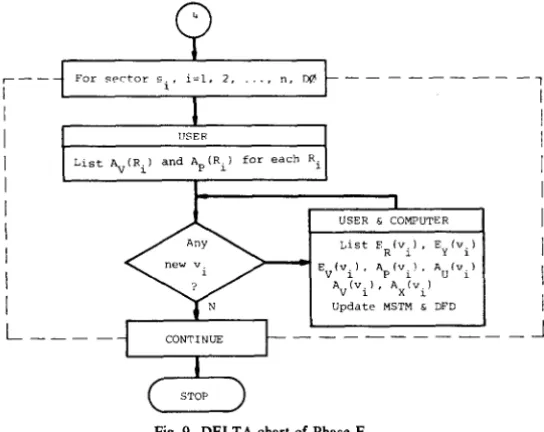
Phase E. In this last phase the affector sets of the rate variables of each sector are identified. From eqn (4) the affector sets of rate variables may be parameters, inputs, auxiliaries and states. The purpose of this phase is to develop the necessary supportive structure within each sector. For each sector, all rates within the sector are inspected for possible supportive parameters and auxili- aries. The user inputs the parameters and auxiliaries through the terminal. For each newly inputted auxiliary vi, the algorithm asks the user to identify existing affector and effector quantities (represented by ER(ui), Ev(ui), Eu(S), Ap(ui), Au(s), Av(ui) and Ah) to

which ui must connect. The MSTM within the

computer’s memory is then appropriately updated. The DELTA chart for this phase is depicted in Fig. 9.

In the next section, each of these phases is further broken down into “steps” and illustrated by means of recourse to a typical textbook example.

AN APPLICATION OF TEE INTEGRATED APPROACH

This section illustrates the concepts of the integrated approach through the use of an example problem. The problem chosen for this purpose is an adapted version of the residential community model discussed on pp. 309-347 of [l l] and patterned after Urban Dynamics[Q The problem addressed by the model is the dynamic inter-

action between population growth and available housing in a residential community such as a resort town. The description of the problem is given below as part of the first step of the integrated approach. The general steps to an integrated approach were discussed by the authors elsewhere [ 191 but a specific algorithm with its particular order and form of queries was not considered. The algorithmatized integrated approach consists of the following steps:

(1) Familiarization with the problem and approach. (2) Determinization of the sectors that comprise the system.

(3) Determination of interaction among sectors. (4) Determination of state-rate interactions within sectors.

(5) Determination of interaction state-rate pairs be- tween sectors.

(6) Determination of between-sector quantities. (7) Determination of within-sector parameters, inputs, outputs and auxiliaries.

(8) Insertion of delays where appropriate.

An integrated approach to the development of continuous simulations 319

c-_zQ

Fig. 9. DELTA chart of Phase E.

E. An iteration through the steps of the integrated ap- proach yields the following results.

Step 1: Familiarization with the problem and

approach. The residential community considered is a

resort town within a fixed geographical area. The population growth in the area depends on the availability of housing as well as the steady natural attractiveness of the area. Natural attractiveness of the area brings people at a certain rate depending on the resident population level as long as the desire for housing matches the availability of houses. Abundant housing attracts people at a greater rate than under normal conditions. The opposite is true when the housing situation is tight. Area residents also leave the community at a certain rate due to various reasons. This outflow of residents also depends on the housing situation.

Housing construction industry, on the other hand, fluctuates depending on the land availability and housing desires. Abundant housing cuts back the construction of houses while the opposite is true when the housing situation is tight. Also, as land for residential develop- ment fills up, the construction rate decreases down to the level of demolition rate of houses.

tAll user-computer conversations depicted in Fig. 10 and following come from an actual interactive user-computer exer- cise. The software employed is documented by Refs. [20] and WI.

ENTER NAME OF SECTOR 1.

housIng

ANY MORE SECTOR NAMES?

Y

ENTER NAME OF SECTOR 2.

population

ANY MORE SECTOR NAMES?

n

Step 2: Determination of the sectors that comprise the system. Figure 10 is an illustration of how the user(s) can converse with the computer program (algorithm) through simple responses to questions from the program. The user answers queries with the information requested. Two sectors or subsystems are identified for the residential community. They are housing (S,) and population (S,). These two sectors delineate a rough boundary for the system considered.

Step 3: Determination of interaction among

sectors. Both sectors affect each other since there is a close relationship between people living in an area and the housing available in the area. There exists a positive feedback loop between the subsystems as shown in Fig. 11. In other words, the housing sector stimulates a larger population sector which further stimulates the housing sector. This structure was elicited from the user by the queries depicted in Fig. 10 below.7

Step 4: Determination of state-rate interactions within sectors. For the housing sector, there is a flow involving houses from new construction to demolition. The number of houses in the area at any time can be ac- cumulated in one level or state variable called simply housing and represented by x1. Symbolically, X1 = {x1 : housing}. The rate variables, R,, that control the flow of houses into and out-of the housing state variable XI are new housing construction rate (rl) and housing demolition rate (rz) respectively. In set notation, R,: the set of rates in sector S, = {r,: new construction rate, r2:

iNTER Y OR N.

ENTER Y OR N.

IN WHAT MANNER DOES HOUSING AFFECT POPULATION ?

ENTER +, -, OR 0.

+

I H WHAT MANNER DOES POPULATION AFFECT HOUSING ?

ENTER +, -, OR 0.

+

MODEL IS BEING STORED.

320 J. R. BURNS and 0. ULGEN

Fig. 11. Interactions between population and housing sectors.

demolition rate}?. Since both of these rates are increas- ing or decreasing the housing stock as a certain percen- tage of the number of houses each year, the state (hous- ing) affects both of the rate variables. These interactions among the states and rates of the housing sector lead to the Dynamo flow diagram. The actual queries asked by the computer during the modeling exercise follow the steps of the Phase B DELTA chart of Fig. 6. A portion of the conversation is delineated in Fig. 13. As each rate is associated with a state, the sign of the coupling is inserted and the current list of the rates is updated for correct state-rate interaction structure within each sector.

In considering the demographic or population sectoi, there is a flow involving people. The number of persons living in the community at any time can be accumulated in one level or state variable. The population state vari- able is represented by x2. Thus X, = {x2: population}. The rates of demographic sector, R2, that control the level of population are the in-migration to the area (r3),

tin the actual computer conversation itself these names were abbreviated to “home cons rte” and “home demo rt” because of a twelve-character name-length limitation in the program.

out-migration from the area (r4) and the net death rate (rs) in the area. The population experiences an annual net death rate due to the largely elderly character of the local population. Symbolically, Rz = {r3: in-migration rate, r4: out-migration rate, r5: net death rate}. These are ab- breviated “in-m&r rate”, “out-migr rte” and “net-death rt” in conversations to follow.

The interactions among the states and the rates of the demographic sector are specified next. Since the rates of this sector increase or decrease the population level as a certain percentage of the population at any time, all the rates of this sector are affected by the population state variable. The MSTM and DFD depicted in Fig. 14 characterize the state-rate interactions for the demo- graphic sector.

Step 5: Determination of interacting state-rate pairs

between sectors. In Step 3, the interactions between

sectors were specified. Generally, all sectors of interest must be coupled with at least one of the other sectors of the system; otherwise, isolated sectors can be in- vestigated separately. The only type of interaction be- tween sectors is the cross-sector state-rate interaction via an information link. This is prescribed by the inter- connection matrix of Fig. 4.

From the problem description, housing x, affects the rates of in-migration r3 and out-migration r.,. Similarly, population x2 has an effect on the housing construction rate r,. Consequently, there are information links in the (xl, r3), (xl, r4) and (x2, rl) positions of the MSTM. Note that at this point there is little concern about whether the cross-sector information links are direct or indirect as this issue will be taken up in the next step. Figure 15 exhibits one possible format for the queries of this step. Queries requesting the sign of the paths are not

I I 1 I

State-rate MSTM of sect”r 1 State-rate DFD of sector 1 Fig. 12. State-rate interactions within housing sector.

CONSIDER SECTOR 1: HOUSING

EI!TER A NE\! STATE NAME FOR SECTOI; l:HOUSING .

housing

APF THERE A?IY MORE STATES IN SECTOR l:HOUSI NG ?

ENTER Y OR N.

”

NAP’E A R4TE (NOT PREVIOUSLY NAMED) VIHICH AFFECTS STATE 1:HOUSING .

home cons rte

DOES 2:HOME CONS RT 4FFECT 1:HOUSING IN A POSITIVE

OP A NEGATIVE MANNER? ENTER + OR -.

+

LIST OF R4TES PREVIOUSLY NAMED.

2: HO:lE COt!S RT

DOES ANY OTHER RATE (NOT PREVIOUSLY NAMED) AFFECT STATE 1:HOUSING ?

ENTER Y of! N.

Y

NAME A R4TE (NOT PREVIOUSLY NAMED) bIHlCH AFFECTS STATE 1:HOUSING .

home demo rt

DOES 3:HOME DEMO RT AFFECT 1:HOUSING IN A POSITIVE

OP A tICGATIVE MANNER? E:ITER + OR -.

LIST OF RATES PREVIOUSLY NAMED.

2: HOF’E CONS RT

3: HOfdE DEMO RT

DOES ANY OT’rER RATE (YOT PREVIOUSLY NAMED) AFFECT STATE 1:HOUSING ?

ENTER Y OR N.

n

An integrated approach to the development of continuous simulations 321

/ -. H-Y

/ c-c \

0

_2k_-

r3

Populatlo"

In-miq. Y'

I Out-miq.

rate

I rate

/

State-rate MSTM of sector 2 State-rate DFD of sector 2

Fig. 14. State-rate interactions within demographic sector.

A PATH EXIST

EI!TFR OR N.

Y

D’JFS A PATH EXIST

ENTER Y OR N.

Y

DOES A PATH EXIST

E’ITER Y OR N.

”

DOES A PATH EXIST

E’ITER Y OR N.

Y

DOFS A PATH EXIST

E’ITER Y OR N.

F7OM 1:HOUSING TO 6C: I N-MIGR RTE ?

FROM 1:HOUSING TO 69:OUT-blIGR RTE?

FROM l:HOUSING TO 70:NET-DEATH RT?

FROM 67:POPULATION TO 2:HOME CONS RT?

FROM 67:POPULATION TO 3:HOME DEMO RT?

”

MODEL IS BEING STORED.

Fig. 15. Conversations related to Phase C (Step 5) for the residential community model.

necessary at this juncture; later when the specific coup-

lings which comprise a path are determined, the sign of these couplings will also be determined.

step 6: Determination of between-sector quantities

(auxiliaries, outputs, parameters and inputs). The pre-

vious step disclosed three between-sector information paths: (x1, r& (x1, r4) and (XZ, r,). In this step of the sector approach the between-sector information paths are each considered separately with the intent of deter- mining if intermittent auxiliaries with adjacent inputs parameters, or outputs are part of the information path. Should this step generate between-sector quantities that are believed to be of types other than auxiliaries, parameters or inputs (such as rates or states), then a new sector will have been identified and the user must return to Step 3. Each of the linkages found in Step 5 are considered separately in the following discussion.

Information link (xl, r3): Effect of housing xl on in- migration rate r3 is indirect through auxiliary variables that specify the condition of the housing market in the area. One quantity which is important is the housing ratio u,. which is defined as the ratio of housing level x1 to housing desired at any time. As available housing begins to exceed housing desired, housing ratio becomes greater than one and the area becomes more attractive for in-migration. The opposite is true when the housing ratio becomes less than one. Since the area attracts a certain in-migration under normal conditions (when ur = 1), housing ratio influences another auxiliary variable (a table function) called attractiveness for in-migration multiplier u2 which in turn increases or decreases the in-migration rate depending on the housing ratio. Thus, between-sector quantities are discovered along the in- formation link directed from housing x, to in-migration rate r3 and include the between-sector auxiliary variables housing ratio u, and attractiveness for migration multi- plier u2. Symbolically, Vb = {u,, u2}. The character of the

queries of this portion of the algorithm is exhibited in Figure 16. The queries enable the determination of direct and indirect linkages, which may coexist in parallel. And, queries within this phase also determine the sign of each coupling.

Let us now consider the quantities in the affector and effector sets of these in-between auxiliaries. Housing ratio u, is affected by housing x, and housing desired u3. Housing desired u3 is a quantity which depends on the current population x2 living in the area and a parameter that specifies housing units required per person p,.

Attractiveness for migration multiplier uz, on the other hand, is influenced only by the housing ratio u,. Symbol- ically, Vb = {u,: housing ratio, u2: attractiveness for migration multplier, Us: housing desired} and PUb = b,:

housing units required per person}. This structure is depicted in Fig. 17(b).

Information link (x,, rd): Effect of housing x, on out- migration rate r4 is again indirect and similar in many ways to the (x,, r3) linkage. Attractiveness of migration multiplier u2 which affects the in-migration rate r3 can be thought of as affecting the out-migration rate r4 if its inverse is taken. The inverse of the attractiveness multi- plier, called the departure migration multiplier u4, regulates the out-migration rate. In other words, as the area becomes more attractive due to favorable effect of housing ratio, more people arrive and fewer people depart than normally. Consideration of the (x,, r4) linkage added one more between-sector auxiliary vari- able, the departure migration multiplier u4, to the set of between-sector quantities so that Qb = VbPbUbVb =

IulrU2,u3,u4>P1~.

Information link (x2, r,): The effect of population

322 J. R. BURNS and 0. UI_GEN

OOFS A PATII EXIST SIKH THAT I:HOUSING DIRECTLY AFFrCTS 6:: IN-:lIGR RATE? ENTER Y OR N.

”

D’IF: ANOTHER PATH (IJOT YET CONSIDERED) EXIST FROM l:HOUSING TO 65: IN-111 G!? RATE? ENTER Y OR N.

Y

Cr)!JSlnEt? TtilS ‘JE’I PATH

NA!tE A NW AW; L;ARY DiRECTLY AFFECTED BY I:HOUSING AND ON THE PATH LEADING TO 68:lN-HIGR RATE.

housni: rat i o

DOES l:HOUSING AFFECT 133:HOUSNG RATIO IN A POSITIVE OR A NEGATIVE MANNER? ENTER + OR -.

+

DOES 133:HOUSNr! RATIO DIRECTLY AFFECT 6s: I N-MIGR RATE? ENTER Y 00 N.

”

:JAb!E A NEll AtJXtLlARY DIRECTLY AFFECTED BY 133:HOUSfJG RATIO AND Or’ THE P4TW LEADING TO 68: IN-illGR RATE.

attract-in

DnFS 133:HQUSNG RATIO AFFECT 134:ATTRACT-IN

O? A NEGATIVE t.IANNER? ENTER + OR -. IN A POSITIVE +

nOFS 134:ATTRACT-IN

EKTER Y OR N. DIRECTLY AFFECT GS:IN-MIGR RATE?

Y

DOES 134:ATTRACT-ItJ

OR A NEGATIVE t.iANNER? AFFECT ENTER + OR 68: I N-MIGR -. RATE IN A POSITIVE

+

;;ES ANOTHER PATH (NOT YET CONSIDERED) EXIST FROM l:HouSt~G fiu0: IN-MIGR RATE? ENTER Y OR N.

”

Fig. 16. A portion of phase D conversations for the residential community model.

Fig. 17(a). System MSTM incorporating X, R and (lb, but not V, PU within the two sectors.

struction multiplier tis which adjusts the normal con- stru~tion rate upward or downward to reflect housing market conditions then is an additional be$ween-sector auxiliary variable (a table function) that links the housing construction rate r, to housing ratio u,.

The system MSTM and DFD incorporating the be- tween-sector quantities is shown in Fig. 17. In the inter- action matrix of Fig. 17 blank entries refer to inferred non-interactions. Zero entries represent situations where non-zero entries could have been inserted without violating the rules of system dynamics but were not because they do not characterize the issue at hand. It is observed that all linkages for the model do occur in those submatrices where, according to the interaction matrix depicted in Fig. 4, linkages can occur.

Sfep 7: ~ie~inution of ~~~~~~-secfor ~~r~me~~rs,

inpufs, outputs and auxiliaries. In this step the necessary support structure within each sector is determined. We proceed by identifying the affector sets of the sector rates. Only auxiliaries, parameters and inputs are brought into the model at this stage and they are further in-

vestigated with respect to their interaction with the other quantities of the sector.

Within the housing sector St, there are two rates pertinent to the sector-housing construction rate rl and housing demolition rate r2. Availability of land is consi- dered of major importance for the housing sector. Hous- ing construction rate r, is affected by the land fraction occupied in such a way that as residential development areas fill up, the construction rate decreases. As long as the Land fraction occupied is low, housing construction rate will follow the normal rate. As a result, we can identify land fraction occupied tr6 affecting the housing construction rate r, through a multiplier called the land av~a~ity multiplier v7. A parameter called normal housing cons~uction p2 specifies the cons~ction rate under normal conditions. Land fraction occupied & is affected by the total residential land p3, land occupied by each house unit p4, and the level of housing xl. Queries transmitted by this portion of the algorithm are depicted in Fig. 18. The selected computer conversation is characteristic of the integrated approach where the type and sign of couplings as well as the type of quantities are generated simultaneously. The algorithm also inter- rogates the user on the existence of alternate paths among quantities. Throughout the modeling exercise, the user has access to the current listings of the affector and effector sets of a given quantity as well as to the list of candidate quantities which may ~tenti~iy affect or be affected by a given quantity.

In considering the other rate of the housing sector, housing demolition rate r2 simply depends on average lifetime of housing p5. The manner in which within- sector quantities of sector S, interact with other quan- tities is prescribed by the sector matrix, Eg. 2. For.this sector invofving 81 pairs, interactions between 54 of them are not possible A consideration of the rem~g 27 (non-blank) pairs leads to the interactions indicated in Fig. 19, where the associated flow diagram is also shown. This completes the structural description for the housing sector S1.

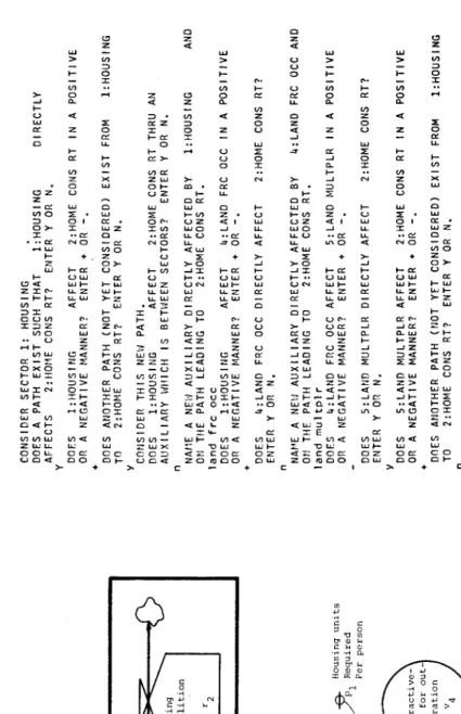
CONSIDER SECTOR 1: HOUSING DOES A PATH EXIST SUCH THAT 1;HOUSlNG OIREC AFFECTS 2:tiOME CONS RT? ENTER Y OR N. ” TLY Housing Construction xl A Demolition Y YY

I

\

\

+ DOES

ANOTHER PATH (NOT YET CONSIDERED) EXIST FROM TO 2:HOME CONS RT? ENTER Y OR N. Y 1:HOUSING CONSIDER THIS NEN PATH. DOES 1:HOUStNG AFFECT 2:HOME CONS RT THRU AN AUXILIARY WHICH IS BETWEEN SECTORS? ENTER Y OR N.

” NAME

A NEN AUXILIARY DIRECTLY AFFECTED BY 1: HOUS I NG AND ON THE PATH LEADING TO 2:HOME CONS RT. z land frc occ 5’ DOES 1:HOUStNG AFFECT 4:LAND FRC OCC IN A POSITIVE OR A NEGATIVE MANNER? ENTER + OR -. 4 + 6 DOES 4:LAND FRC OCC DIRECTLY AFFECT 2:HOME CONS RT? CL ENTER Y OR N.

s P

n NAt’E

A NEll AUXILIARY 01 RECTLY AFFECTED BY 4:LAND FRC OCC AND

a

ON THE PATH LEADING TO 2:HOME CONS RT. a- land mu1 tpl r 8 DOES 4:LAND FRC OCC AFFECT 5:LAND MULTPLR IN A POSITIVE OR A NEGATIVE MANNER? ENTER + OR -. w DOES 5:LAND MULTPLR DIRECTLY AFFECT 2:HOME CONS RT? ? ENTER Y OR N. E Y ?i DOES 5:LAND MULTPLR AFFECT 2:HOME CONS RT IN A POSITIVE OR A NEGATIVE MANNER? ENTER + OR -. B + % DOES ANOTHER PATH (NOT YET CONSIDERED) EXIST FROM l:HOUStNG 8 TO 2:HOME CONS RT? ENTER Y OR N.

z. 2 z

” LIST OF KNOWN AFFECTORS OF 2:HOME CONS RT 1: HOUSING 5: LAND MULTPLR 2. 137: CONS MULTPLR LIST OF POSSIBLE AFFECTORS OF 2:HOME CONS Rl 4: LAND FRC OCC IS 2:HOME CONS RT DIRECTLY AFFECTED BY ANY OF THE POSSIBLE AFFECTORS? ENTER Y OR N.

n DOES

ANY UNNAMED V,P, OR U DIRECTLY AFFECT 2:HOME CONS RT? ENTER Y OR N.

Y NAME

A NEIJ V, P, OR U. const r norm IS 6:CONSTR NORM AN AUXILIARY? ENTER Y OR N.

n DOES

324 1. R. BURNS and 0. ULCEN

*~$Fq~y

Fig. 19. Structural description for the housing sector, including V, PU.

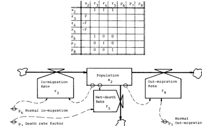
rates; namely, in-migration rate r3, out-migration rate r4, and the net death rate r5. Normal in-migration p6 and normal out-migration p, are the parameters affecting in-migration rate and out-migration rate under normal conditions-i.e. when housing desired equals the housing available. Similarly, the net death rate at the community depends on another parameter, death rate factor pS,

which is constant due to the age structure of the resi- dential community population. The interactions are determined from a consideration of the sector matrix, Fig. 2. The resultant matrix and associated DFD are shown in Fig. 20. For this sector, 34 of the 49 possible pairs are inferred as noninteractant (all which are blank

in Fig. 20). Thus only 15 pairs (those which are nonblank) permit interactions consistent with the rules of system dynamics.

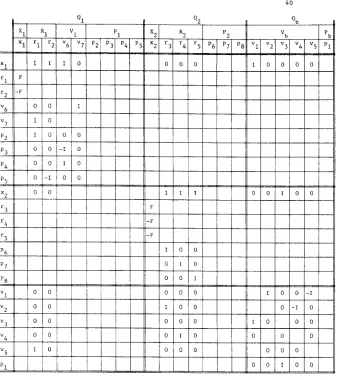
The computer would utilize the previously obtained information about the problem of interest to complete the interaction matrix depicted in Fig. 4. The resultant interaction matrix for the example problem is shown in Fig. 21 together with the associated flow diagram. Blank entries were inferred, while zero entries represent situa- tions where interactions were feasible but nonetheless not representative of the problem considered.

Step 8: Insertion of delays where appropn’ate. An examination of information links in the models shows the

An integrated approach to the development of continuous simulations 325

II 92 0 ‘b _I

“3 0 0 0 0 0 I 0 0 0

I

"4 0 0 1 0 IO 0 0 0

"5 I Oi 0 0 0 0 0 0

I

Pl I 0 0 10 0

Fig. 21(a). Complete interaction matrix for residential community model

existence of a perception delay between the attractive- ness and in-migration variables. An increase (decrease) in attractiveness of the area will be perceived with delay by the people outside the community. Adding this delay to the Dynamo flow diagram of Fig. 21 essentially completes the Dynamo flow diagram component of the computer-aided model formulation exercise.

SUMMARY AM) CONCLUSION

In this paper an innovative approach to the develop- ment of continuous simulations is described. Fundament- ally, the new approach is premised upon the presumption that, through computer assistance, the procedure for simulation model formulation can be expedited, syste- matized, and operationalized. The computer-aided ap- proach is derived from the assertions of causality im- plicit within Forrester’s system dynamics. If implemen- ted, the approach will likely motivate and facilitate the determination of the important sectors, the important quantities to be included, the existence of couplings between the quantities, as well as the identities of both couplings and quantities. A systematic formulation process may produce models which would enjoy a greater degree of credibility and validity. Equally im- portant, such models could be developed quickly.

SEPS Vol. 12. No. CC

Computer-internalized models could also be analyzed and tested for stability, reachability, observability and controllability by means of algorithms. All these plati- tudes remain to be proven in empirical model formula- tion exercises utilizing computer-assistance, however.

326 J. R. BURNS and 0. ULGEN

---+ \I t

Population

In-migration AA x2 O"t-"1qratlan

Pate ry Y- Rate

r3

\

Net-death \ I4

,--__'

l \ _.- 1' Rate \

r5

1-N I j

A- p6 Normal In-migration / /

A' I

,---___- NO-1

Death rate factor ‘a, Out-miqratlon

Fig. 21(b). Dynamo flow diagram for completed residential community model.

(blanks), thereby preventing errors of commission to occur in which a link which is incompatible with the rules of system dynamics is inserted.

An overview algorithm was thereafter presented and discussed. The approach was then illustrated through recourse to a classical textbook example-the residential housing model-found in [ll]. The approach was found to produce a model that was consistent with the classical textbook example. In this example the specific form of queries posed by software already available[20,21] was indicated. The procedure and queries were both found to be quite compatible with the concerns of modelers who employ system dynamics methodology.

Acknowledgemen?-The authors are indebted to Mr. H. W. Beights who translated sketchy flow charts and theoretical developments into a formal algorithm and associated software.

REFEBENCES

1. G. Fromm, W. Hamilton and D. Hamilton, Federally Supported

Mafhemoricol Models: Survey and Analysis, National Science 2.

3.

4.

5.

Foundation-RANN publication number NSF-RA-S-74-029 (available from U.S. Government Printing Ofice. Washington, DC. 20402, #038-OOO-OO221-0), 1974.

Ways to Improve Management of Federally Funded Compu- terized Models, National Bureau of Standards, Number LCD 75-111, 1975.

J. R. Burns, A preliminary approach to automating the process of simulation model synthesis. Proc. of the 7th Ann. Pittsburgh Conf. on Modeling and Simulation, p. 820 (1976).

J. R. Burns, Converting signed digraphs to Forrester sche- matics and converting Forrester schematics to differential equations. IEEE Trans. on Systems, Man and Cybernetics, SMC-7 (W77).

R. Fitz and D. Hornbach, A participative methodology for designing dynamic models through structural models. Proc. of the 7th Ann. Pittsbqh Conf. on Modeling and Simula- tion, p. 1168 (1976).

J. W. Forrester, Industrial Dynamics. M.I.T. Press, Cambridge (1961).

J. W. Forrester, Principles of Systems. Wright-Allen Press, Cambridge (1%8).

An integrated approach to the development of continuous simulations 321

9. J. W. Forrester, World Dynamics. Wright-Allen Press, 16. A. Thesen. Some notes on systems models and modeling. Inf.

Cambridge (1977). J. Systems Sci. 5, I45 (1974).

10. N. B. Forrester, The Life-Cycle of Economic Development. 17. W. Wakeland. A low-budget heuristic approach to modeling Wright-Allen Press, Cambridge (1973). and forecasting. Technological ForecastinK and Social

11. M. R. Goodman, Study Notes in System Dynamics. Wright- Change 9 (1976).

Allen Press, Cambridge (1974). 18. J. Warfield. Societal Systems. Wilev. New York (1976).

12. F. Harary, R. Norman and D. Cartwright, Srrucrural Models: 19. J. R. Burns and 0. Ulgen, A sector approach to the formula-

An Introduction to the Theory of Directed Graphs. Wiley, tion of system dynamics models. Inr. .I. Systems Sci. (1978)

New York (1965). 20. H. W. Beights, Computer Aided Simulation Methodology,

13. J. Kane. A primer for a new cross impact language-KSIM. CASMI, User’s Guide, Tech. Rep. QT-111-78, Department

Technological Forecostina and Social Change 4. 129 (1972). of Industrial Enaineerina. Texas Tech Universitv. Lubbock, 14. G. J. Klir, An Approach to General Systems Theory. Van Texas, 1978. - I

Nostrand, New York (1969). 21. H. W. Beights, Computer Aided Simulation Methodology, 15. R. H. Mall and C. M. Woodside, TR No. S.E. 76-l. Systems CASMI. Programmer’s Guide, Tech. Rep. QT-I 12-78.

Engineering Department. Carleton University, Toronto, Department of Industrial Engineering, Texas Tech Univer-