The Generalised Extreme Value Distribution
as Utility Function
DENIS CONNIFFE*
National University of Ireland, Maynooth, Co Kildare
Abstract: The idea that probability distribution functions could provide appropriate mathematical forms for utility functions representing risk aversion is of respectable antiquity. But the relatively few examples that have appeared in the economics literature have displayed quite restrictive risk aversion properties. This paper examines the potential of the generalised extreme value (GEV) distribution as utility function, showing it possesses considerable flexibility as regards risk aversion properties, even in its single parameter form. The paper concludes that the GEV utility function is worth considering for applications in cases where parametric parsimony matters.
I INTRODUCTION
T
he economics and finance literature contains many papers on useful mathematical forms for utility functions for income or wealth. For such functions to embody risk aversion, the first derivative must be positive and the second derivative negative, and it is usually convenient that the functions be positive. In at least some applications parsimony of parameters is also desirable – the familiar Bernoulli utility u(x) = log x has none at all. Probability distribution functions are positive, have positive first derivatives – the probability densities – and if they are unimodal, have negative second derivatives beyond the mode. Some distributions are quite parsimonious in275
*I am grateful to an anonymous referee for helpful suggestions.
parameters, especially if location and scale parameters are set to zero and unity respectively. The potential of distributions to serve as utilities was appreciated by Berhold (1973) who illustrated with the cases of exponential and normal distributions. Lindley (1976) extended the examination to utilities derived from the somewhat more general single parameter exponential family.1A few other examples of distribution functions used as utilities can be found in the economic literature, for example, the logistic distribution was employed by Filho, Suslik and Walls (1999), but there are not very many.2 There are also some examples of implicit or indirect employment of distribution functions in obtaining utilities. The “Leyden” approach to elicitation of peoples’ welfare or utility through simple questions about how they perceive their personal situations (Van Praag, 1968; Van Praag and Kapteyn, 1973) relies on assuming an equivalence of a welfare or utility measure to a cumulative distribution.
Of course, distribution functions cannot represent the whole class of utility functions. Some very popular utility functions, such as the logarithmic or positive power forms,3 are unbounded and cannot be scaled to distribution functions. There can also be limitations in terms of flexibility or convenience to employing some distributions as utility functions. It is easily shown that some imply increasing absolute risk aversion (IARA) over the whole range of income or wealth, a property also associated with the quadratic utility function. Because of the perceived implausibility of this property, textbooks tend to dismiss quadratic utility and the same would presumably apply to the employment of these distributions as utility functions. Again, many distribution functions, including the normal, cannot be expressed in a closed form, even if they can be evaluated numerically. While the familiarity of the normal may make it the exception,4most economic researchers would consider it inconvenient not to have explicit algebraic expressions for their utility functions.5
1Both Berhold and Lindley also considered the expectations of these utilities with respect to
selected wealth distributions, utilising results on the conjugate distributions of Bayesian statistics.
2 There are some examples in other literatures of distributions as utilities, although not
necessarily in a risk aversion framework. Chen and Novick (1982) employed truncated normal and beta distributions to represent the utilities of educational outcome scores. LiCalzi and Sorato (2006) considered the Pearson family of distributions as potential utilities and demonstrated a connection to HARA (hyperbolic absolute risk aversion) type utility functions.
3That is u(x) = (xλ– 1)/λ with 0 λ < 1.
4The normal distribution function under the title ‘Error Function’ has long featured in texts on
mathematical functions, for example, Abramowitz and Stegun (1970).
5However, recent work by Meyer (2007) argues that very often the derivative of the utility
The purpose of this paper is to examine the potential of the Generalised Extreme Value (GEV) distribution function to serve as a utility function. In recent years the GEV has become increasingly familiar in economics, and particularly in financial econometrics, because of its role in quantifying the probabilities of extreme falls in the value of financial funds. Properties of the GEV have been intensively studied6including its use in prediction as have the approaches to estimating parameters. It has a very simple closed form expression, although this can be seen as comprising a family of three distributions, sometimes called the Type I Extreme, or Gumbel; the Type II Extreme, or Frechet; and the Type III Extreme, or reversed Weibull, distributions. The GEV involves a single shape parameter and optional location and scale parameters. As will be seen, even in its most parsimonious parameterisation, it possesses appreciable flexibility as regards risk aversion properties, including the capacity to embody such features as subsistence and saturation levels of consumption.
II THE GEV UTILITY FUNCTION
The single parameter GEV distribution is
u(x) = exp
–(1 – kx)k– 1 . (1)If kis positive, it is evident that for u(x) to be real x< 1/kand u(x) attains its maximum value of unity at x= 1/k. This corresponds to the fact that the Type III extreme value distribution is bounded above. The derivative of the utility is
u'(x) = exp
– (1 – kx)k– 1 (1 – kx)1 –1k– ,which is real and positive, given the already stated condition. The second derivative is
(1 – k)– (1 – k)k– 1 u"(x) = –u'(x) –––––––––––––––(1 – kx)
and this is clearly negative for k 0. For kpositive, kmust be 1 and
1
x> – [1 – (1 – k)k] (2)
k
Clearly the right hand side of (2) is the mode xMof the GEV distribution, where the derivative of the density is zero. The valid range of x, if u(x) is to represent risk aversion, must lie to the right of the mode. For k < 0 the right hand side is negative so there is no difficulty as xmust be positive. If k = 0, L’Hospital’s rule shows the right hand side is zero.7For kpositive, xhas lower and upper bounds given by
1 1 – [1 – (1 – k)k] < x< – k k
[image:4.499.75.434.380.581.2]The lower bound could be interpreted as a subsistence level of income or wealth, where utility equals exp (k – 1), and the upper bound as a saturation level, where utility is unity. When k = 1, the GEV distribution becomes a reversed exponential ranging from –∞ to 1 and mode at 1, so the interval between bounds shrinks to the point x= 1. It is probably often realistic that utility exists for all positive x, so that k 0 is the more practically important case, but subsistence and saturation levels can sometimes be relevant.
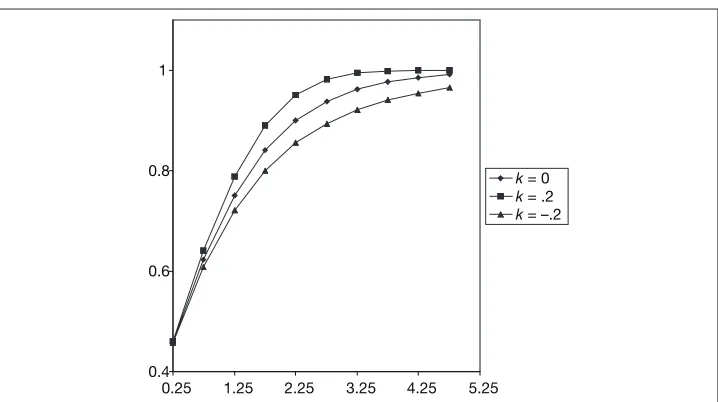
Figure 1: GEV Utility Functions
7For k= 0 the GEV distribution (1) takes the Gumbel form u(x) = exp {– exp(– x)} because the limit
as ngoes to ∞ of (1 – y/n)nis u(x) = exp (–y). 0.4
0.6 0.8 1
Figure 1 shows the utility functions for k = –.2, k = 0 and k = .2. The concavity increases with k, showing that for fixed x, aversion to risk rises with k. For k = .2 the maximum utility of unity is reached at the finite value of x= 1/k, which is the saturation level and is 5 in this case.8For k= 0 unity is not reached at any finite value of x, but clearly the value attained at x= 5 is very near it. For k = –.2 the utility attained is appreciably below unity, which corresponds to the fat upper tail property of the Type II extreme value distribution.
The Arrow-Pratt coefficient of absolute risk aversion –u"(x)/u'(x) is
(1 – k) – (1 – kx)k– 1
RA= ––––––––––––––––––––– (3)
(1 – kx)
or 1 – exp (–x) at k= 0. Its derivative is
k(1 – k) + (1 – k)(1 – kx)k– 1
R'A= ––––––––––––––––––––––––––––––– (1 – kx)2
and this is positive for positive k, implying IARA. It is easily seen that RA increases from zero at the subsistence level to infinity at the saturation level. Since the coefficient of relative risk aversion RRis defined as x RA, increasing relative risk aversion (IRRA) must also hold.
For the probably more frequently relevant case of knegative, R'Abecomes zero for
1 1
x0= —
–––– – 1. (4)k kk
When x< x0, R'Ais positive and when x> x0, R'Ais negative. For k –1, x00 and so x, being positive, exceeds it. Therefore, decreasing absolute risk aversion (DARA) holds throughout. For –1 < k < 0, x0, takes a positive value. Then IARA holds for 0 < x x0and DARA holds for x0< x< ∞. As x → ∞it is clear that RA→ 0.
For fixed x, the derivative of RAwith respect to kis
x– 1 + (1 – 1/k)(1 – kx)k– 1
––––––––––––––––––––––––––––– (1 – kx)2
8 The value of 5 may seem to be very restrictive, but units of measurement can be chosen
which is positive for k negative (at least for x > 1) so that the larger the k for an individual or group the less risk averse they are at constant x.
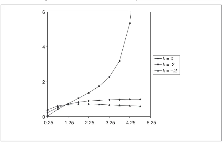
[image:6.499.73.435.198.431.2]So, for a single parameter utility function, the GEV can display consider-able flexibility regarding absolute risk aversion properties. Depending on choice of k, IARA and DARA can occur, as can cases displaying a transition from one to another and also subsistence or saturation levels can feature. Figure 2 illustrates how the absolute risk aversion changes with x.
Figure 2: Absolute Risk Aversion of GEV Functions
A brief comparison with the distribution functions that have appeared previously as utility functions is worthwhile. The normal distribution as utility function has
1 u'(x) = —––– e–x2
2π
leading to RA= xand IARA. Again, the logistic distribution
1 u(x) = —–—
1 + e–x gives
2 RA= 1 – —–—
1 + ex
0 2 4 6
implying IARA. The exponential distribution of course gives the constant absolute risk aversion (CARA) case, which, if perhaps sometimes more acceptable than IARA, is still inflexible.9
The GEV function is not fully flexible, at least in the single parameter form, where relative risk aversion is concerned. For k negative the coefficient of relative risk aversion is, from (3)
(1 + k) – (1 + kx)– —k
1
RR= –––––––––––––––––– (k+ 1/x)
As xincreases the denominator decreases and the numerator increases. So IRRA holds for all xand knegative as well as positive. As x → ∞ it is evident that RR→ 1 + 1/k. In fact, for very large k and any xthat is not small, RR is effectively unity.
III ADDING LOCATION AND SCALE PARAMETERS
A location parameter β and a scale parameter α, which must be positive, can be added to (1) by replacing xby (x– β)/α giving
x– β k– 1
u(x) = exp
–1 – k––––– . αIt will be shown that this modification can increase flexibility properties. However, it should be said straightaway that if multi-parameter utility functions are permitted, there are already some very flexible functions in the literature10 and it is doubtful if any utility functions derived from distributions with the same number of parameters can improve on them.
If kis positive x< β + α/k is now required to avoid imaginary numbers. As the mode has clearly been pulled to the right (assuming β positive) to
α
xM= β+ – [1 – (1 – k)k] k
9It might be objected that, as presented, these distributions have no parameters, so comparisons
of flexibility with the one parameter GEV are unfair. But adding location and scale parameters μ and σ to the normal or logistic makes no difference to their IARA property, nor does introducing a scale parameter to the exponential alter its CARA property.
10For example, Xie’s (2000) power risk aversion utility function and Conniffe’s (2007)
the lower and upper bounds for x, defining the subsistence and saturation levels, are now given by
α α β+ – [1 – (1 – k)k] < x< β+ –.
k k
Even if k is negative it is no longer certain that x can range from zero because xMmay be positive and
α
x > β– — [1 – (1 + k)–k] (5)
k
if it is to exceed the mode.11 So there can be a subsistence level even with k negative.
Letting z = (x – β)/α it follows that u'(x) = u'(z)/α and u"(x) = u"(z)/α2. So u"(x) negative requires k < 1 as before. Since RA(x) = RA(z)/α and R'A(x) = R'A(z)/α2, R'
A(x) is positive when R'A(z) is. Since R'A(z) is always positive if kis, IARA holds for all xfor positive k. For negative k, R'A(z) is zero for z0given by (4), so R'A(x) is zero for
α 1 x0= β+ —
—– – 1.k kk
When x< x0, IARA holds and when x > x0, DARA holds. Turning to relative risk aversion
x x β+ zα β
RR(x) = xRA(x) = – RA(z) = — RR(z) = —––— RR(z) =
1 + —RR(z). α zα zα zαNow, although it follows from Section II, that RR(z) increases with z, 1 + β/(zα) clearly decreases with z and so there may be possible ranges of x where decreasing relative risk aversion (DRRA) holds. The existence and extent of the relevant range depends on the values of the parameters k, α and β. For example, for k= –1 it can be shown that
2 α 2x 2αx
RR'(x) = –––––––– – ––––––––––– – ––––––––––– + ––––––––––– (6) (α– β) + x [(α– β) + x]2 [(α– β) + x]2 [(α– β) + x]3
11Note that even with k negative imaginary numbers would arise unless x> β– α/k. However,
Since x must be positive and exceed the mode, here β – α/2, the lower bound for xis zero if β< α/2 and is the mode if β > α/2. Then, as it is easily verified that
α– 2β α 8 α R'R(0) = –––––– and R'R
β– –= —β– –,(α– β)2 2 α2 2
IRRA must hold initially as xincreases. Now the first and third terms of (6) are O(x–1), while the second and fourth are O(x–2). So for large xthe sign of R'R(x) depends on that of
2 x –––––––––
1 – –––––––––. (α– β) + x (α– β) + xThe term in square brackets is positive if α> βand negative if α< β. So in the latter case the initial xinterval of IRRA is followed by an interval where DRRA holds.
Overall though, the flexibility of the relative risk aversion properties of the GEV utility are not too impressive. Since any possibility of DRRA derives from 1 + β/(zα) decreasing with z, it cannot occur if β = 0 is zero. But, as was mentioned earlier, if β is non-zero the mode xM could be positive even with negative kso that the utility function is not available for all positive x. Indeed, even the example just discussed shows that β may need to be considerably greater than zero for a substantial interval of DRRA to exist. While a possible subsistence level at non zero xis sometimes a useful feature, it will often, as previously mentioned, be plausible that a utility be defined for all positive x. It seems restrictive to limit DRRA to utilities incorporating a subsistence level.12This tends to confirm the earlier suggestion that if several parameters are permitted, existing functions in the literature may be superior to distribution functions, or at least to the GEV.
IV PLAUSIBILITY OF GEV DISTRIBUTION FOR REPRESENTATION OF UTILITY
Arguments for the plausibility of various functional forms for utility can (approximately) be grouped into three classes. The first considers how the mathematical features of the function accord with the economic properties
12The GEV utility would not be alone in doing so, however. The three-parameter HARA utility
considered desirable in a utility. The second draws on psychological and physiological considerations to explain why individuals may possess particular forms of utility functions. The third class assesses the empirical evidence for the success of various functions in applications.
Commencing with the desirable properties of utility functions, there is not full consensus about these features beyond the two fundamentals that utility should be monotonically increasing in wealth and that the rate of increase should be decreasing (the concavity property).13 Arrow (1971) felt a utility function should display DARA and IRRA, arguing the plausibility of regarding a risky asset as a normal good and not an inferior one. IARA would imply holdings of risky assets would decline with increasing wealth. From Sections II and III is it clear that GEV utility can meet these conditions for a wide range of parameter values. The fact that it might not do so for some parameter values is not a disadvantage, as it permits testing the hypotheses through parameter estimation. Arising from analysis of the role of the utility function (with consumption as argument) in explaining precautionary savings, Leland (1968) deduced that an appropriate function should have a positive third derivative (the “Prudence” property). This is no difficulty with the GEV for a wide parameter range. Indeed, if the third derivative was not positive DARA could not hold. Other authors who have argued the plausibility of even further limitations on utilities include Pratt and Zeckhauser (1987), Kimball (1993) and Caballe and Pomanski (1996) and their required restrictions can also be satisfied by the GEV utility. Of course, the GEV utility is not alone in satisfying these conditions. So do many other utilities including the very popular power function.
The second class of plausibility arguments are possibly more fundamental, but perhaps even more debatable. They focus on how individuals form their impressions of the welfare, or utility, they derive from their wealth. In behavioural psychology there is a field of “psychophysics” dating back to the nineteenth century researchers Weber and Fechner, which examines such issues as the relationship of physiological stimulus to sensation. Drawing on this material Sinn (1983, 1985) argued for logarithmic or power forms for utility functions. Various papers by other authors have also supported log utility, some of the more recent drawing on findings in the field of evolutionary psychology. Of course, these arguments do not support distribution functions as utilities, but other psychology-based arguments can be made that do.
One is based on arguing that utility is really a relative rather than absolute measure. The idea is that someone would perceive more utility from
13Even the concavity property has sometimes been disputed. For example, the Friedman-Savage
the same wealth if in a low income community than in a high income one. Perceived utility of an individual’s wealth is determined by position in the community’s income distribution, that is, by the proportion of the population with lower income. So there is a direct equivalence between the utility function and the cumulative distribution of income. The idea is not particularly recent in economics as it was employed by Gregory (1980) and is also related to the “Leyden” approach mentioned in Section I. Of course, there are difficulties if the equivalence is actually applied to the whole income distribution, because then (assuming the distribution unimodal) the lower income side is convex, implying risk-loving behaviour at lower incomes.14The concavity condition can be maintained by taking the equivalence to be between utility and the distribution “translated” to its mode as origin. Since income distributions are usually described as positively skew with long right hand tails, the GEV distribution with k 0 would seem appropriate. So too, of course, would other distributions such as lognormal, Weibull and Pareto (when lower incomes are ignored). There are other themes in psychology related to choice of utility function. The random utility model of Luce and Suppes (1965) treats a person as possessing a mental distribution of utility functions, one of which is selected at random when making a decision.15 In behavioural economics individuals are sometimes considered as being composed of ‘multiple selves’ (for example, Thaler and Shefrin, 1981) and a referee has suggested that perhaps this currently popular approach could provide a justification for GEV utility. GEV distributions arise as limiting distributions for the largest value in a sample and perhaps the extreme value drawn from the distribution of ‘multiple selves’ captures utility. Unfortunately, this author does not know enough about behavioural economics to properly assess and develop this suggestion.
These arguments based on psychophysical or psychological considerations are rather contradictory as regards utility function formulae. In addition, the various formulations apply to the individual and it is not clear how they might extend to the ‘representative consumer’ underlying much of economic analysis. So it would be very useful if the third class of arguments, concerning empirical evidence of successful application, could clarify matters. There are two difficulties here. First, relatively few utility functions (and certainly not the GEV) have been widely employed. By far the most commonly used are the simple single parameter CARA exponential form or the CRRA
14Gregory did apply the correspondence to the whole distribution, because he wanted to provide
some plausible support for the Friedman-Savage (1948) utility function.
15Manski (2001) relates this model to McFadden’s (1974) use of random utility to analyse discrete
power (or log) form. The second difficulty is that since utility is not directly observable, the plausibility of the utility function has to be judged by how well some model for observable variables fits the data. But a poor fit could well be attributable to the failure of model assumptions quite unrelated to the utility function.
Consumption theory in macroeconomics can serve as an example. A power function for the utility of consumption, which is very convenient mathe-matically, has dominated in the huge volume of research, both theoretical and empirical. But there are some problems, including the famous ‘equity premium puzzle’ where the intertemporal consumption model seems incompatible with the observed differences in returns from stocks and bonds. Some authors, for example Meyer and Meyer (2005), have seen the inflexibility of the power utility as a possible explanation for the puzzle and felt that its replacement by another function could provide a resolution of the puzzle. However, many other explanations have also been put forward for the puzzle and so it is unclear just how much the validity of power utility may have been undermined. More generally, Xie (2000) has discussed the dangers implicit in choosing power utility arising from the possibly inappropriate implication of CRRA. He illustrated his argument by discussing analysis of cross-country diversity in growth rates, showing how an incorrect CRRA assumption could lead to spurious differences obscuring understanding and arguing for a much more flexible utility function. Of course, weakening support for power utility does not necessarily strengthen the case for GEV utility, but it at least justifies examination of it as one of a set of alternatives.
REFERENCES
ABRAMOWITZ, M. and I. E. STEGUN, 1970. Handbook of Mathematical Functions, New York: Dover.
ARROW K., 1971. Essays in the Theory of Risk Bearing, Amsterdam: North-Holland. BERHOLD, M. H., 1973. “The Use of Distribution Functions to Represent Utility
Functions”, Management Science,Vol.19, pp. 825-829.
CABALLE, J. and A. POMANSKI, 1996. “Mixed Risk Aversion”, Journal of Economic Theory, Vol. 71, pp. 485-513.
CAMPBELL, J. Y. and J. H. COCHRANE, 1999. “By Force of Habit: A Consumption-based Explanation of Aggregate Stock Market Behaviour”, Journal of Political Economy,Vol. 107, pp. 205-251.
CHEN, J. J. and M. R. NOVICK, 1982. “On the Use of a Cumulative Distribution as a Utility Function in Educational or Employment Selection”,Journal of Educational Statistics,Vol. 7, pp. 19-35.
COLES, S., 2001. An Introduction to the Statistical Modelling of Extreme Values, New York: Springer-Verlag.
CONNIFFE, D., 2007. “The Flexible Three Parameter Utility Function”, Annals of Economics and Finance,Vol. 8, pp. 57-63.
EMBRECHETS, P., C. KLUPPELBERG and T. MIKOSCH, 1998.Modelling Extremal Events for Insurance and Finance, New York: Springer,
FILHO, F. N., S. B. SUSLICK and M. R. WALLS, 1999. “Managing Technological and Financial Uncertainty: A Decision Science Approach to Strategic Drilling Decisions”, Natural Recourse Economics,Vol. 8, pp. 193-203.
FRIEDMAN, M. and L. P. SAVAGE, 1948. “The Utility Analysis of Choices Involving Risk”, Journal of Political Economy, Vol. 56, pp. 279-304.
GREGORY, N., 1980. “Relative Wealth and Risk Taking: A Short Note on the Friedman-Savage Utility Function”, Journal of Political Economy, Vol. 88, pp. 1226-1230.
KIMBALL, M. S., 1993. “Standard Risk Aversion”, Econometrica, Vol. 61, pp. 589-611. LELAND, H. E., 1968. “Saving and Uncertainty: The Precautionary Demand for
Saving”, Quarterly Journal of Economics,Vol. 82. pp. 465-473.
LiCALZI, M. and A. SORATO, 2006. “The Pearson System of Utility Functions”,
European Journal of Operations Research, Vol. 172, pp. 560-573.
LINDLEY, D. V., 1976. “A Class of Utility Functions”, Annals of Statistics, Vol. 4, pp. 1-10.
LUCE, R. and P. SUPPES, 1965. “Preference, Utility and Subjective Probability” in R. Luce, R. Bush and E. Galenter (eds.), Handbook of Mathematical Psychology,
Vol. 3, New York: Wiley.
MANSKI, C. F., 2001. “Daniel McFadden and the Econometric Analysis of Discrete Choice”, The Scandinavian Journal of Economics,Vol. 103, pp. 217-229.
MCFADDEN, D., 1974. “Conditional Logit Analysis of Qualitative Choice Behaviour” in P. Zarembka (ed.), Frontiers in Econometrics, New York: Academic Press.
MEYER, D. J. and J. MEYER, 2005. “Risk Preferences in Multi-period Consumption Models, the Equity Premium Puzzle, and Habit Formation Utility”, Journal of Monetary Economics. Vol. 8, pp. 1497-1515.
PRATT, J. W. and R. J. ZECKHAUSER, 1987. “Proper Risk Aversion”, Econometrica,
Vol. 55, pp. 143-154.
SINN, H-W., 1983. Economic Decisions Under Uncertainty, Amsterdam: North-Holland.
SINN, H-W., 1985. “Psychological Laws in Risk Theory”, Journal of Economic Psychology,Vol. 6, pp. 185-206.
THALER, R. F. and H. M. SHEFRIN, 1981. “An Economic Theory of Self-control”,
Journal of Political Economy, Vol. 89, pp. 302-406.
VAN PRAAG, B., 1968. Individual Welfare Functions and Consumer Behaviour,
Amsterdam: North Holland.
VAN PRAAG, B. and A. KAPTEYN, 1973. “Further Evidence on Individual Welfare of Income: An Empirical Inquiry in the Netherlands”, European Economic Review,
Vol. 4 , pp. 32-62.