The slow equations : Part I: Derivation and properties of the system / Part II: Application to continuous data assimilation

METEOROLDGICRL SERVICE

TECHNICAL NOTE No.

50

THE

SLOW

EQUflTIONS

Part

I:

Derivation and Properties of the System.

Part

JI:

Application t o Continuous Data Assimilation.

BY

Peter Lynch. M.Sc., Ph.D.

UDC

551.509.313

Price

E5.25

The race is not always t o the swift; slow and steady is sure t o win.

Abstract

A

filtered system o f equations is derived. using the ideas o f normal mode initialization. This

&

eouation system models the low frequency

rotational atmospheric motions: there are no solutions corresponding t o gravity

waves. The prognostic element o f the system is an equation expressing the

conservation of potential vorticity. The slow equations d i f f e r from the general

balance system a t second order in the Rossby number. and are free from the

spurious solutions found in that system. Integration o f a barotropic model with

the slow equations shows them t o be highly accurate compared t o the primitive

equations.

Since the slow system is noise-free. it may be useful f o r continuous

data assimilation. The slow equation model is free from data shock, and adjusts

immediately t o inserted data. The balance equation, a component o f this

system, may be used t o define local balance so t h a t inserted data projects

onto the rotational. modes, thus ensuring that a perturbation of given

magnitude is assimilated by the model.

Table o f

Contents

PART I : Derivation and P r o ~ e r t i e s o f the System.

2 .

DERIVATION OF THE SLOW EOUATIONS. 2a. Background.

2b. Derivation o f the Slow Equations.

3 . THE SLOW EOURTIONS AN0 THE BALANCE SYSTEM.

3a. Introduction.

3b. Perturbation Expansion.

3c.

The Transition between the t w o Systems.

3d. Linear Normal Modes.

38. Thompson's 'Minimally Filtered' Model.

3 f . R General Filtered System.

4. NUMERICAL INTEGRATION OF THE SLOW EOUATIONS.

4s. Discretization.

4b. The Lagrangian Timestep. 4c. Diagnostic Steps.

5 . COMPARISON WITH A PRIMITIVE EOUATION MOOEL.

6 . INlTlALlZRTION AN0 THE SLOW SYSTEM.

INTERMEZZO

I . GEOSTROPHIC ADJUSTMENT.

la. Rn Equation f o r the Rsymptotic Solution.

Ib. The importance o f Mass

5

Wind Data. Ic

.

Consequences f o r Data Rssimilation. Id. The Rate o f Rdjustment.

PART 11: Application t o Continuous Data Assimilation.

7 .

ASYNOPTIC ORTR ASSIMILATION

-

GENERAL CONSIDERATIONS. 7a. Introduction.

7b. Rnalysis. Data Escalation. 7c. Rssimilation and Data Shock.

7d. Review o f t h e Laplece Transform Scheme.

8. DATA INSERTION EXPERIMENTS.

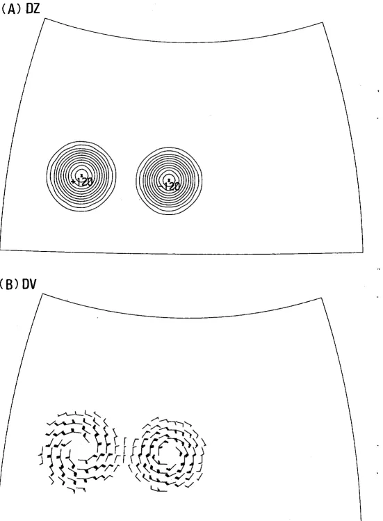
Ba. Description o f a Perturbation.

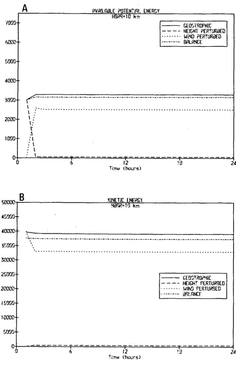
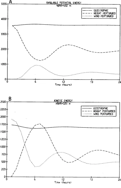
Bb. Preliminary Perturbation Experiments. Bc. Energy Response and Rate o f Rdjustment. Bd

.

Perturbing Realistic Background Fields. Be. Balanced Winds.

9. SUMMARY OF RESULTS.

Thanks

1 am grateful t o my colleagues Ray Bates. Jim Hamilton and Aidan McDonald f o r numerous illuminating discussions, and t o

1

.

INTROOUCTION.

The object of Numerical Weather Prediction is t o forecast the

evolution of the slow, rotational motions of the atmosphere. The high

frequency gravity waves which are also solutions of the primitive equations

have been causing headaches f o r modellers ever since Richardson's (1922)

pioneering forecast. The f i r s t successful numerical forecasts by Charney e t a/.

(1950) circumvented the problem by filtering the equations so that only the

slow motions remain as solutions. However. the resulting quasi-geostrophic

equations were not always sufficiently accurate, so a return was soon made t o

using the primitive equations. Since these equations support gravity waves.

forecasts made with them may be very noisy unless the initial data reflect the

balance between the mass and wind fields found in the atmosphere. Modification

of the data t o ensure this balance is called initialization.

A

more direct attack on the noise problem would be t o develop a filtered system which simulates the rotational flow eccurately but is free from

gravity waves. Using the ideas o f normal mode initialization, Daley (1980)

devised a system in which the low frequency components o f the flow are

forecast, while appropriate gravity wave components are diagnosed a t each

moment. This system proved t o be highly accurate when compared t o a

primitive equation model. Combining Oaley's approach with the implicit normal

mode method of Temperton (1985). it is possible t o express this system in

terms o f the physical variables (obviating the need f o r transformations t o and

from normal mode space). We shall call the resulting system the

&

eouations.

1 I

The balance equations are based on assumptions less drastic than

those leading t o the quasi-geostrophic system, and should therefore be more

accurate. Oaley (1982) has constructed a non-iterative procedure f o r

integrating the balance system, and his results confirm i t s high accuracy. R

recently by Thompson (1980). However, the general balance system admits

spurious non-physical solutions ( w i t h phase speeds f a r in excess o f the gravity

wave speed) in addition t o the rotational modes (Moura, 1976).

The slow equations may also be deduced by means o f scaling

arguments similar t o those used t o derive the balance system, and based on

smallness o f the Rossby number. Ro. Both systems are accurate up t o O ( R O ~ ) ,

and may be expected t o yield r e s u l t s o f comparable accuracy. There is a

difference a t O(RO') between the systems, w i t h the consequence t h a t t h e

slow equations are f r e e f r o m t h e spurious unphysical solutions.

The slow system has one prognostic component, t h e equation o f

conservation o f potential v o r t i c i t y . This equation is in a f o r m ideally suited t o

t h e application o f the semi-Lagrangian method o f integration. The diagnostic

elements o f t h e system may be w r i t t e n as standard Helmholtz equations, whose

solution is s t r a i g h t f o r w a r d . Parallel runs show t h e slow system t o be very

accurate when compared t o a primitive equation model. When used w i t h a zero

timestep (i.e.. omitting the semi-Lagrangian step) t h e slow system can be

used t o initialize data f o r a primitive equation run. This is precisely the implicit

normal mode method o f initialization (Temperton, 1985. Juvanon du Vachat,

1986).

This r e p o r t is in t w o p a r t s : P a r t I. outlined above, deals w i t h t h e

derivation o f t h e slow system, i t s properties and some t e s t integrations t o

establish the accuracy o f the system: P a r t II deals w i t h the use o f the system

f o r continuous data assimilation. In between, there is a section devoted t o the

theory o f geostrophic adiustment, which is relevant t o P a r t 11. The r e s u l t s

here are standard, b u t t h e equation f o r the adjusted s t a t e is derived using

Laplace t r a n s f o r m theory. This technique automatically incorporates t h e initial

conditions in an equation f o r t h e final s t a t e , and is perhaps more convenient

than the conventional approach.

One o f the major problems in continuous data assimilation is t h e

generation o f spurious gravity wave noise. In P a r t I1 we discuss t h i s problem

and p e r f o r m several simple experiments w i t h the primitive and slow systems.

The slow equations provide a suitable means f o r the assimilation o f

observational data during a forecast, as they can absorb inserted data without

s u f f e r i n g high frequency shocks. Furthermore, t h e i r response t o inserted data

i s immediate, whereas the response o f the primitive equations may be very

slow if the adjustment time-scale is long. This instantaneous response is a

g r e a t advantage if data is t o be inserted frequently. The general balance

equation is an inherent component o f t h e slow system, and it may conveniently

be used t o define a local balance when data is inserted. in such a way t h a t

perturbations o f given magnitude (i.e. in agreement w i t h observations) are

assimilated by the system.

I I

An alternative method o f f i l t e r i n g and data assimilation was discussed

by Lynch (1906). In this method the Laplace t r a n s f r o m technique is used t o separate components purely on t h e basis o f frequency, and t h e r e is more

control (over which modes are retained and which ones f i l t e r e d o u t ) than w i t h

a system such as t h e slow equations.

F u r t h e r investigation is needed before a choice between the t w o

methods can be made. Moreover, the choice will undoubtedly depend upon the

specific details o f t h e envisaged application.

This r e p o r t leaves a number o f important questions unanswered. Two

particularly vital issues are t h e accuracy o f t h e slow system in a baroclinic

context, and i t s practical u t i l i t y f o r data assimilation in an operational setting.

The f i r s t issue is essential t o the ability o f the slow equations t o simulate

phenomena such as f r o n t a l development. It is hoped t o examine t h i s question

and present the r e s u l t s in a f u t u r e r e p o r t . We also hope t o apply the slow

equations t o the assimilation o f hourly synoptic data. Because o f t h e properties

o f the system. t h e r e a r e grounds f o r optimism; b u t f u r t h e r discussion here

2. OERIVRTION OF THE SLOW EQUATIONS.

2a. Background.

Daley (1980) has used the ideas o f normal mode initialization t o

develop a method o f integrating the primitive equations efficiently. The original

equations can be w r i t t e n

where X is the s t a t e vector o f unknowns. L is a constant linear operator

( m a t r i x ) and N is a nonlinear vector function. When transformed t o Hough-mode

space, the system splits into t w o subsystems:

Where

Y

and

2

are respectively t h e coefficients o f t h e slow and f a s t components o f the flow and Ay, AZ a r e diagonal matrices o f eigenfrequencies.

..

Machenhauer ( 1977) proposed t h a t

(2)-(3)

could be initialized by s e t t i n g the tendencies o f t h e f a s t modes t o zero. Assuming Machenhauer's c r i t e r i o n

(2

=

0)

t o hold throuqhout the inteqration, Oaley replaced (2)-(3) by t h e system

giving a prognostic equation f o r the slow modes and a diagnostic equation f o r

the f a s t modes. I will call ( 4 ) - ( 5 ) the Slow Equations (in normal mode f o r m ) .

Using the slow equations, Daley developed an integration scheme which was

stable, e f f i c i e n t and accurate: he compared a r u n w i t h the slow equations and

A t = 40 min. t o a control r u n w i t h the primitive equations and A t =

I0

min. ; the

r m s differences in surface pressure and SO0 hPa winds a t 48 hours were only

(per timestep) in Daley's scheme is due t o the transformations between

spectral (spherical harmonic) space and normal (Hough-)mode space: f o r a

gridpoint model the transformations would be even more expensive.

Temperton (1905) has devised an initialization scheme which is

completely equivalent t o the normal mode method, but which operates in

physical space. A very similar method has been presented by Juvanon du Vachat

(1986). The central idea o f Temperton's approach is t o choose a linearization

and t o reformulate the physical equations so t h a t the tendencies can be

separated b y i n s ~ e c t i o n into slow and f a s t components:

Using Machenhauer's criterion,

4

=

0

a t t =

0,

Temperton derived an initialization scheme which he called t h e implicit normal mode method; the same approach will

be used here t o derive

a

system o f slow equations in physical space.

In the following section we will use the ideas o f Daley and Temperton

t o develop a system o f equations equivalent t o t h a t o f Daley, b u t formulated in

terms o f the physical variables. The integration o f this system does n o t

require any transformations between physical and spectral space; nor does i t

require knowledge o f the linear normal modes o f the model being integrated.

2b. Derivation o f the Slow Equations.

A general baroclinic system o f equations may be separated, by transformation t o the vertical eigenmodes, into a number o f systems equivalent

t o the shallow water equations. Therefore, we consider the shallow water

where N Nd and N, represent the nonlinear terms. d o t s denote local time

<'

derivatives and otherwise the notation is conventional. The Coriolis parameter f

is variable, b u t the 8-terms are included on the right-hand side. We assume

t h a t f = f(x.y) depends upon b o t h horizontal coordinates (as it does f o r a polar

stereographic projection o r f o r r o t a t e d latitude/longitude coordinates) and

denote i t s derivatives by

p,

and

By.

Then the nonlinear t e r m s a r e

The v o r t i c i t y and continuity equations may be w r i t t e n

and f r o m these we easily derive an equation expressing t h e conservation o f

potential v o r t i c i t y

Expanding the time derivative and keeping only linear t e r m s on the l e f t , this

may also be w r i t t e n in the f o r m

This equation may alternatively be derived directly f r o m (7) and ( 9 ) .

Although

(7)-(9)

are n o t separable, we can easily deduce some

have zero linearized potential vorticity (Il=

C8<-f@l).

Property

C A I

is easily

seen by considering stationary solutions o f the system

(7)-(9).

Property

CBI

follows f r o m ( 1

1

). linearized so t h a t the r h s vanishes, and the f a c t t h a t the f a s t modes must have nonzero frequencies. These properties imply t h a t t h e

tendencies o f divergence and (geostrophic) imbalsncs ( E *

C V ~ @ - ~ < I )

project

entirely onto t h e f a s t modes, and the tendency o f potential v o r t i c i t y entirely

onto t h e slow modes:-

These a r e the explicit f o r m o f ( 6 ) above. An equation f o r the tendency o f the

geostrophic imbalance is easily derived f r o m (7) and

(9):

This imbalance equation. together w i t h

(8)

and

(10)

( o r

( I I)),

gives a system

o f three equations completely equivalent t o the original system ( 7 ) - ( 9 ) .

We now assume t h a t the qravity

-

wave ~ r o i e c t i o n s o f tendency

vanish. Thus, the tendency t e r m s in

( 0 )

and

(15)

are dropped: the potential

-

v o r t i c i t y equation

(10)

is l e f t unchanged. The resulting system is

We shall call this system the

Slow

Epuations. They are equivalent t o Oaley's

equations

(4)-(51,

b u t r e f e r t o t h e physical variables. obviating the need f o r

The above analysis may be repeated w i t h the p - t e r m s included in the

linear analysis (Juvanon du Vachat, 1987: Temperton, 1987). The resulting

equations are a l i t t l e more cumbersome, and it is unclear whether any

advantage is obtained ( c f . Lynch. 1985, sac. 4). Similarly, the t o t a l

derivatives o f 6 and e may be omitted, r a t h e r than t h e i r local tendencies:

Thompson (1980) argues t h a t t h i s i s a physically more meaningful approximation.

It amounts t o replacing Machenhauer's f i l t e r i n g c r i t e r i o n by an alternative:

Machenhauer:

8

= 0. Alternative: = 0. d t

Again. the r e s u l t is a somewhat more complicated f o r m o f t h e nonlinear terms.

It i s n o t clear whether t h e alternative approximation yields b e t t e r results.

Finally, Tribbia (1984) has developed a higher order method o f initialization.

Rather than assuming t h a t t h e nonlinear t e r m s in

( 3 )

a r e constant, he

represents them by low order polynomials in time. The f i r s t - o r d e r version o f

his technique is the same as Machenhauer's method. The second-order version

consists o f setting t o zero t h e second (time-) derivative o f the gravity

modes:

a t

-

Machenhauer:

_{a t}

=

0.

Tribbia (2nd order) :

-

0.

We could use Tribbia's c r i t e r i o n t o derive slow equations o f higher order: any

practical advantages would have t o be weighed against the added complexities o f

3. THE SLOW EOUATIONS AND THE BALANCE SYSTEM.

3a. Introduction.

The slow equations a r e similar, b u t n o t identical, t o the general

balance system. There is a single prognostic variable, the potential v o r t i c i t y .

Various small t e r m s are retained in t h e slow equations which are nurmally

dropped in the balance system. However, the most important difference is the

omission o f the tendency o f (geostrophic) imbalance (;) in the slow equations.

This may be justified by scaling arguments similar t o those which lead t o the

balance system.

The essential approximation in deriving the balance system i s the

replacement o f the divergence equation by a diagnostic relationship between the

stream function and the geopotential. The resulting system o f equations is

highly implicit, and i t s numerical solution presents some difficulties (Charney.

1962; Daley, 1982). The general balance system admits spurious high-frequency solutions in addition t o t h e Rossby wave solutions (Moura. 1976): it will be shown below t h a t the slow equations are f r e e f r c m t h i s problem.

3b. Perturbation Expansion.

We consider t h e shallow water equations, linearized about a s t a t e o f

r e s t :

We introduce length and velocity scales L and V, assume an advective time scale

L/V and scale 0' geostrophically as 2OLV. The nondimensionalized f o r m s o f

( 1 1 4 3 ) then become

where p = s i n

9.

Ro = (V/20L) is the Rossby number and F r =

v2/8

is the Froude number. The v o r t i c i t y and divergence equations become

where a = c o s # and a is the e a r t h ' s radius.

We assume t h e following values f o r the scale f a c t o r s . e t c .

Then the nondirnensional numbers take values as follows:

We have assumed t h a t L < a so t h a t (L/a) = O(Ro). This is t r u e f o r synoptic

scales o f motion; f o r planetary scales L a, and the scaling must be

reexamined (Burger, 1958).

.'

We will now derive perturbation forms o f t h e equations, c o r r e c t up

The expansions are substituted into the equations of motion and terms of like

order in Ro are equated. We perform the expansion process in two different

ways: the conventional method leads t o the balance system: and a reformulated

method, starting from equivalent but different forms o f the original equations,

yields the slow equations.

Method A. We expand equations

(a),

(9)

and (10). The zeroth-order terms give

representing nondivergent, geostrophically balanced flow. Next, we consider the

terms o f order Ro, which give

In dimensional form, the equations correct up t o order

O ( R ~ )

are

This is the conventional (linearized) balance system. We note that there are

two prognostic equations, and w i l l show below that this leads t o spurious

solutions of the system in addition t o the Rossby wave solutions.

We have assumed that

L a a

and L/a = O(Ro), which is true f o r synoptic scales. Since 6, vanishes. the wind field may be partitioned into

Thus, in the @-terms o f CBEI the winds may be replaced by their rotational

components. The equations are then equivalent t o t h e linearized f o r m o f

Charney's (1962) equations (5.1-3). For planetary scales the full winds must

be kept (Charney. 1973). It is the inclusion o f the t e r m

pu,

in CBE(iii)l which

leads t o t h e spurious solutions (Moura. 1976).

Method 0.

W e

now define t h e imbalance as

and observe f r o m the foregoing analysis t h a t

With an advective timescale appropriate t o low frequency motions we expect

t h a t the tendency o f

is

also small. From (I). (3) and (4) we easily deduce:

In nondimensional form this becomes

and we recall t h a t ~ 0 ~ ~ r - l =

o(1)

Consider the system o f equations (4).

(5)

and ( 1 1 ) or, in nondimensional f o r m (9). (10) and ( 12). The dependent variables a r e expanded

as before and coefficients o f like powers o f Ro considered together. The zero

which represents nondivergent geostrophically balanced flow, as before. Now

the f i r s t order t e r m s give the following system:

In dimensional f o r m the equations c o r r e c t up t o O(Ro2) are

( i i ) CSEl

(iii)

This system is denoted CSEl as it is a f o r m o f the Slow Equations, o f t h e

same character as as those derived in the previous chapter. The f i r s t t w o

equations a r e identical t o those which were obtained above f o r the CBEI

system. However, we now have a diagnostic equation f o r 6 in place o f the

continuity equation. There i s only one prognostic component, and the only

normal modes a r e the Rossby waves

-

the system is f r e e o f spurious modes. This f a c t , together w i t h the e x t r a simplicity o f the system, makes it more

a t t r a c t i v e than the conventional balance system.

3c. The Transition between the t w o Systems.

Since b o t h the systems CBEI and CSEI have been derived f r o m the

same s t a r t i n g point, w i t h the same scaling assumptions, and since b o t h are

c o r r e c t a t ~ ( R O ) , any differences between them must be O(Ro2) a t most. We

will show now t h a t t h i s i s the case.

From [BE] it is s t r a i g h t f o r w a r d t o derive the equation

a

2

s(V

0-fr)

+

( G V ' - ~ ~ ) ~

-

fpv = 0. (3.13)

scaling this equation as before. i t appears immediately t h a t t h i s tendency t e r m

vanishes a t the zeroth and f i r s t orders in Ro. But the removal o f the t e r m

renders the balance and slow systems identical. Therefore, they are equivalent

a t O(Ro).

Despite the difference between [BE1 and CSEI being only

O ( R ~ ) .

t h e r e is no direct means o f transition between them. Considering [BE1

psr E.

the tendency t e r m in (13) must be kept. To make the transition we must take

a step backwards t o the original primitive system. The presence o f t h e

tendency t e r m in (13) is a fundamental difference between t h e balance and

slow systems, and justifies d i f f e r e n t names being given t o them.

3d. Linear Normal Modes.

Since t w o time derivatives a r e omitted in the slow system CSEI. the

dispersion relation is linear in the frequency. There is only a single normal mode

f o r given wavenumbers. The balance system [BE1 has t w o time derivatives; a

naive argument would suggest t h a t the system should have a quadratic

dispersion r e l a t ~ o n and t h e r e f o r e admit modes other than the Rossby wave

solutions. L e t us examine t h i s in more detail.

The system [BE], w r i t t e n in t e r m s o f the stream function and

velocity potential. is

Seeking solutions o f the f o r m A.expCi(kx+ly-vt)l we get a quadratic dispersion

relation:

2 2 2

where K = (k + l and a ( = 1 or 0) is a t r a c e r indicating inclusion o r exclusion o f

If a = 1 and we define cR

=

-p/K2

and cG = 4(b+?/K2). t h e phase speed c = v / k

must satisfy

Since l c R l alc61. the second t e r m in t h e linear coefficient may be omitted. The

t w o r o o t s may easily be found approximately: f o r i c l small we omit the

quadratic term. arriving a t

which is t h e familiar Rossby wave speed; f o r i c l large t h e constant t e r m is

dropped, giving

Since\cGlw lcR(, this solution is much f a s t e r than a gravity wave. It is in f a c t a

spurious solution. w i t h no physical significance. Such physically unrealistic high

frequency. eastward-propagating solutions were discussed by Moura (1976).

Our naive reasoning has proved correct: t h e t w o time derivatives in

t h e balance system give r i s e t o t w o types o f normal mode solution. If the

t e r m

pux

is dropped f r o m the balance equation. we p u t a=O and the quadratic

t e r m in the dispersion relation ( 1 4 ) disappears. Then t h e only solution is t h a t

having t h e Rossby wave speed, and the system is f r e e o f spurious solutions. In

general, t h e condition necessary t o avoid spurious solutions IS t h a t the balance

equation have no t e r m involving a divergence element ( 1 , u x , v x o r 6).

3e. Thompson's 'Minimally Filtered' Model.

Thompson (1980) has re-examined the minimum approximations leading

t o the complete exclusion o f gravity waves. He modifies t h e divergence equation

by omitting the t o t a l time-derivative o f divergence, obtaining a rninimallv

component o f t h i s system must be satisfied by modification o f the initial data.

The model is a generalization o f the balance system. Thompson has proposed a

method o f integration, b u t does n o t present any numerical results.

Thompson's central argument is t h a t the omission o f the tendency o f

divergence is both necessary and sufficient f o r the elimination o f gravity wave

solutions. In this sense the slow equations would appear t o involve unnecessary

approximations, in t h a t the tendency o f (geostrophic) imbalance is also

omitted. Yet, t h i s tendency projects entirely onto the gravity wave

components. as we have seen above (Eq (2.13)). Thus, i t s omission can hardly

be deleterious t o the accuracy w i t h which t h e slow system models the

rotational modes. Furthermore. since Thompson's system contains t w o

prognostic equations, the v o r t i c i t y and continuity equations, it admits spurious

high frequency solutions (unless f u r t h e r approximations are made; Thompson

omits the p - e f f e c t , b u t in general i t would have t o be included). The t h i r d

equation is a diagnostic relation f o r t h e divergence; if t h e continuity equation

is replaced by the balance equation, the r e s u l t is (essentially) the slow

system.

We will see below t h a t the difference between a f o r e c a s t w i t h the

slow equations and a reference r u n w i t h a primitive equation model is about the

same size as the e r r o r s obtained by Daley (1982) using the balance system. As

the t w o systems yield r e s u l t s o f comparable accuracy, t h e slow equations may

be considered t o have a clear advantage by v i r t u e o f t h e i r greater simplicity

and the absence o f unphysical solutions.

3 f . fl General F i l t e r e d System.

The foregoing analysis was applied t o t h e linear shallow water

equations - 3 A similar approach may be used in a more general nonlinear

where E , the imbalance, is the sum o f all remaining terms. Now we derive an

equation f o r the r a t e o f change o f 6 , which may be w r i t t e n formally as

The derivation o f this equation may be algebraically involved. Thompson (1980)

has derived an expression f o r q which includes t h e e f f e c t s of nonlinear

advection (although the @-terms are omitted). Note t h a t (17) may also be

w r i t t e n

To obtain a aeneral f i l t e r e d system, we omit t h e time derivatives in

(16) and (17). (Either partial o r t o t a l time derivatives may be omitted;

Thompson (1980) argues t h a t only the t o t a l derivatives have intrinsic physical

meaning, being independent o f the coordinate system). Equation (16) now becomes a generalized balance equation, expressing the relationship between the

mass and rotational flow fields. Equation (17) becomes a diagnostic equation

f o r the divergence (analogous t o the omega equation); we may call it the

imbalance eauation, since i t is the approximate f o r m o f t h e equation f o r the

tendency o f imbalance. We complete the system by adding the equation f o r

conservation o f potential vorticity. The full f i l t e r e d system may then be

w r i t t e n

(PV conserved)

E = O (Balance Eqn. )

q = O (Imbalance Eqn.

This is the general slow system. With a single prognostic component, it models

the slow. rotational motions and is f r e e f r o m both gravity waves and spurious

Hinkelmann (1969) proposed a general method f o r defining initial data

f o r the primitive equations. He suggested t h a t the observed wind and mass

fields should be adjusted so t h a t

d d2

-( 0.V) = 0 and

dt.

(0.V) = 0.

d t (3.20)

That is, these t w o conditions should be used t o derive diagnostic relationships.

which could then be used t o f i l t e r the initial data. Cls an alternative, he

pointed out t h a t these conditions could be used t o replace t w o prognostic

equations by

diagnostic

relationships, yielding a general filtered system: this is precisely what we have done above. Thus, the slow equations are an

Implementation o f t h e filtering technique

originally

suggested by Hickeimann. It was f u r t h e r argued by Hinkelmann t h a t an improved balance would

be achieved by requiring

d" dnr'

-( 0.V) =

C

and

-

(0.V) = 0.

dt" dtW'

f o r n > 1. We can re-express these criteria as

Clearly, f o r n = 2

order initialization

n

d r = O

dt" dt"

these a r e essentially the same as Tribbia's ( 1 9 8 4 second

technique. Likewise, there is a correspondence between the

procedures f o r larger n.

It

is evident t h a t higher order systems o f slow equations could be derived by using (21) r a t h e r than (20). t o derive diagnostic

4. NUMERICAL INTEGRATION OF THE SLOW EOURTIONS.

The numerical integration of the slow system is straightforward. We

rewrite the system (2.16-2.18) here f o r convenience:

The potential vorticity equation ( 1 ) is in a form ideally suited t o the

semi-Lagrangian approach. This method ensures unconditional stability f o r the

time integration. which is a great advantage. After each timestep, the

diagnostic relationships

(2)

and (3) are used t o calculate the remaining

variables. Certain quantities not known a t the new time must be

&&.

or

evaluated using values from the previous time. The error thus incurred could

have been reduced by an iterative procedure, but this was found t o be

unnecessary. The method used bears some similarity t o the non-iterative

method used by Daley (1982) t o solve the balance equations.

4s. Discretization.

The only prognostic variable is the potential vorticity

ll

=

(<+f>/O.

Since it is convenient t o calculate and 0 a t the same points, a 0-grid is

used, with v calculated a half gridstep east and

u

half a gridstep north o f

each @-point. A single grid cell thus appears as follows

The grid covers the area shown in Figure 5.1. There are 40x26 points with a

spacing of 2'x2' on a rotated latitude/longitude grid with pole a t 1 5 0 ~ ~ . 30'~.

The initial data is the (uninitialized) operational analysis of

mean height calculated f r o m this analysis is 5439 metres. The wind fields were

interpolated f r o m a C- t o a D-grid. Calculation o f the vorticity

<,

and thence

n,

a t @-points gives us the s t a r t i n g values f o r the integration.

4b. The Lagrangian Timestep.

The prognostic element o f the slow system is equation (I).

expressing conservation o f potential vorticity. To integrate this equation, we

use a t w o time-level semi-Lagrangian technique. Thus. ( 1 is approximated by

3 t time

- t i c i t y ll a t the gridpoir

where the potential vor (n+l)At is equal

t o i t s value a t a departure point, denoted by an asterisk, a t time nbt. The

departure point is estimated using a technique described by McDonald and Bates

(1987). This technique uses centering in both time and space. and bilinear

interpolation. With the departure point thus estimated. the value o f

n

a t this

point a t time nAt is calculated by a bicubic interpolation, and by (4) this

immediately gives us the value a t point

(1.J)

a t the new time. The

semi-Lagrangian method is discussed more fully in Bates and McDonald (1982).

4c. Diagnostic Steps.

From (2) and the definition o f il. we get an equation f o r the

geopotentiai :

The nonlinear r i g h t hand t e r m s are calculated using values a t nAt, except f o r Il

a t ( n + l ) A t . Note t h a t the coefficient o f @ on the r h s is small, so t h a t the

resulting time truncation e r r o r should also be small. Then 0"" is obtained by solution o f the Helmholtz equation (5). We use SOR f o r simplicity. although

faster methods a r e available (see Appendix o f Temperton, 1987). From

nnil

and

The next step is t o compute

N(

and N, and then the right hand side

of

( 3 )

using the most up-to-date values available. This Helmholtz equation is

then solved f o r the divergence 6*'.

The winds a t time (n+l)At must be retrieved from the vorticity and

divergence fields. This process requires the specification of a single wind

component on the boundary. In the method of Sangster (1960) the stream

function and velocity potential are calculated by solving two Poisson equations.

and the wind is then deduced from them. A more direct method (Lynch, 1907).

requiring the solution of only one Poisson equation. yields equally accurate

results and was used in this study.

Finally. the vorticity is recalculated in order t o agree with the wind

values specified on the boundaries, and ll is recomputed. Point values and global

averages o f various quantities. energy components and other diagnostics are

calculated and stored a t each timestep. A t the end of the integration the

winds are transformed back t o a C-grid t o allow direct comaprison with a

5. COMPARISON WITH R PRlMlTlVE EOURTION MODEL.

To assess t h e accuracy o f t h e slow equations. a series o f parallel

runs using slow and primitive equation models was c a r r i e d out. The slow

equation model CSEI is as described in section 4 above. The primitive e q u a t i ~ I

model CPEI is a one-level version o f t h e model described by McDonald (1906). It

uses a semi-Lagrangian advection scheme and a semi-implicit adjustment step.

The grids are identical f o r t h e t w o models, except t h a t CPEl uses a C-grid.

whereas CSEI uses a 0-grid, so t h a t

u

and v points are interchanged.

Rs a reference run, we take t h e CPEI 24 hour f o r e c a s t w i t h a

timestep A t = 10 minutes. The initial analysis o f height is shown in Figure

5.1 ( a ) , the 24 hour f o r e c a s t in Fig. 5.1 ( b ) and t h e difference in Fig. 5. l ( c ) .

To limit gravity wave noise in t h e primitive equation model, a light divergence

damping is applied, w i t h a coefficient velue Z~IO' m2s-I (Sadourny. 1975). This

damps out t h e noise in about 12 hours.

Preliminary runs w i t h t h e CSEI model d i f f e r e d significantly f r o m t h e

reference, suggesting c e r t a i n changes. The average divergence was t o o high.

and t h e r e were large differences between t h e runs near t h e western boundary.

To counteract t h e f i r s t e f f e c t . t h e divergence was s e t t o zero on the

boundary p r i o r t o t h e solution o f (4.3). This resulted in a reduction o f the

-6 -I -8 -I

r m s divergence f r o m 1.8a10 s t o a more reasonable value 5.7r10 s

.

The large

differences near t h e western boundary were due t o a discrepancy in t h e

t r e a t m e n t o f t h e boundary conditions. To remove this.

5

and

ll

were recalculated a f t e r r e t r i e v a l o f t h e winds a t each timestep. This led t o more

compatibility between t h e t w o models.

R f t e r these adjustments, t h e differences between t h e reference r u n

and t h e CSEI model w i t h a 10 minute timestep were very small. The difference

between t h e height f o r e c a s t s had an rrns value o f only 5.9 metres and a

maximum difference o f 20 metres; the difference field is shown in Figure 5.2.

differences are smaller than typical observational errors.

Both models are capable o f being integrated with long timesteps.

since they both use stable numerical schemes (the operational 3-0 version o f

[PEI uses a timestep o f 90 minutes). To investigate t h e time truncation

e r r o r s , both CPEI and CSEl were r u n w i t h a one hour timestep, and the

results were compared t o the corresponding runs with A t = 10 minutes. For

[PEI t h e r m s differences in height and winds were 5.8 metres and 0.9 m/s.

For

CSEl

the relevant figures were 3.6 metres and 0.5 m/s. These differences a r e small enough t o suggest t h a t t h e e r r o r s associated w i t h a one hour

timestep are quite tolerable in both cases. Thus, all f u r t h e r integrations

discussed were made w i t h a 60 minute timestep f o r both

CPEI

and CSE].

The e f f e c t s o f t w o d i f f e r e n t methods o f retrieving t h e winds f r o m

t h e vorticity and divergence were examined. We made t w o parallel 24 hour

forecasts, using the method o f Sangster (1960) and the direct method o f

Lynch (1987) t o r e t r i e v e t h e winds a t each timestep. The same normal

boundary winds a t t h e same gridpoints were used in each case. The r m s

difference between the forecast wind fields a f t e r 24 hours was only O.l3m/s;

the height fields d i f f e r e d by less than one metre. For all practical purposes,

the forecasts were identical.

A

full description o f the t w o methods is given in Lynch (1987).

.

s

*

The results o f t h e comparison between t h e primitive and slow

equation models presented above indicate t h a t the slow equations are capable of

accurately modelling t h e low frequency rotational components o f t h e flow.

which are o f primary meteorologicai significance and interest. The question o f

how the slow equations may simulate baroclinic systems, and small scale

systems such as f r o n t s , is o f fundamental importance, and must be examined

6. INITIALIZATION

AND

THE SLOW SYSTEM.

The data f o r a primitive equation model must be initialized if spurious

gravity wave noise is t o be avoided. In the CPEI model, t h e divergence damping

reduces this noise a f t e r about 12 hours, b u t there is a severe initial shock and

large unrealistic oscillations during t h e early forecast hours. The slow equations

have no solutions corresponding t o gravity waves, and are f r e e o f these

problems. The diagnostic components o f the system automatically ensure t h a t a

balance between the mass and wind fields is maintained a t all times. In this

sense, the slow equetions a r e self-initializinq. The CSEI model may also be used

t o initialize the data f o r t h e primitive epuation model. However. the evolution

o f the flow in the CSEI f o r e c a s t is smoother than t h a t o f CPEI, even when

the l a t t e r s t a r t s f r o m initialized data.

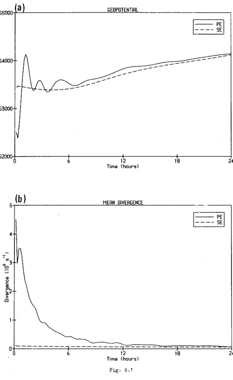
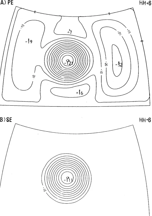
The d i f f e r e n t character o f the flow evolution produced by the

primitive and slow models is clearly shown in Figure 6.1. The graph

6 .

l (a)

shows t h e height a t a central point (I=19.J=9) plotted against time. The noisy

character o f the IPEI f o r e c a s t is abundantly clear, and is in sharp c o n t r a s t t o

the smooth curve resulting f r o m the CSEI integration. R similar p l o t o f mean

divergence, shown in Figure 6. l (b). confirms the noisy character o f the CPEI

run. and f u r t h e r demonstrates how the slow system produces a smooth

evolution, f r e e o f the initial shock and subsequent noise.

The slow equations may be used t o initialize the data f o r the CPEI

model. This is done by integrating t h e initial data, using CSEI, f o r one or more

timesteps. b u t w i t h A t = 0. i.e. omittinq the semi-Laqransian s t e ~ . This is

completely equivalent t o t h e implicit normal mode method o f initialization

(Temperton. 1985: Juvanon du Vachat. 1986). The number o f 'zero' timesteps

is equivalent t o the number o f iterations o f the normal mode technique. In

practice, t w o iterations a r e s u f f i c i e n t t o initialize the data. Forecasts f r o m

uninitialized data are denoted by NIL, and those f r o m data a f t e r t w o zero

The evolution o f the height field a t a central point CI=26.J=12) f o r

t h e CPEI model without and w i t h initialization are shown in Figure 6.2(a). The

absence o f an initial shock in the NL2 run is clear. However, there is evidence

t h a t some high frequency oscillations remain. In Figure 6.2(b) t h e NL2 r u n is

replotted with an expanded vertical scale ( i t is denoted PRIM), together with

t h e values forecast by t h e CSEI model (denoted SLOW).

It

is clear t h a t the l a t t e r produces a smoother evolution. The residual noise in CPEI was not

removed by f u r t h e r iterations o f the initialization. Use o f a higher order

scheme (Tribbia, 1984) might well remove this noise. However, there seems t o

be an inherent tendency f o r t h e CPEI model t o produce some high frequency

components. It seems possible t h a t the residual noise in Figure 6.2(b) is

associated w i t h the boundaries: t h e area is approximately 5000 km across, and

a gravity wave with a phase speed o f 300 m/s would cross it in about

5

hours;

this is about the same as the period o f the noise.

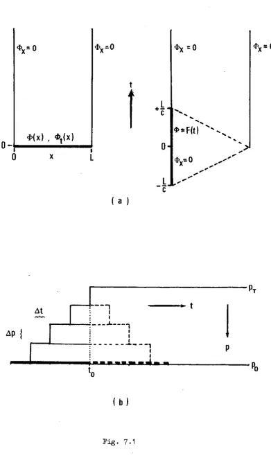
In Table 6.1 t h e differences between the uninitialized and initialized

runs a t various stages are presented. The differences a f t e r 24 hours are

significantly smaller than the initial changes. These r e s u l t s are broadly

comparable t o the results using the Laplace transform technique o f initialization

(Lynch. 1985. Table 2 ) .

*

*

*

The complete absence o f high-frequency noise f r o m t h e CSEI forecast

may be o f great advantage if t h e model is t o be used f o r data assimilation.

The insertion o f observational data which is not completely compatible w i t h the

forecast s t a t e may give r i s e t o large oscillations in a primitive equation model.

The resulting noise causes problems f o r subsequent data induction cycles. The

slow equation model should be f r e e f r o m these problems. The process o f

52000

0

6

12

18

Time (hours)

[image:34.592.45.511.73.833.2]

I

b 12 ! 9

Time thours)

I

b 12

'9

Time ( h c ~ r s )

[image:35.591.53.522.83.802.2]

TABLE 6.1. Root-mean-square (and maximum) differences in height and wind between the original and Initialized fields (NL2 mlnus NIL) and between the 12 and 24 hour forecasts resulting from these flelds.

Fore-

[image:36.596.177.502.134.348.2]

INTERMEZZO: GEOSTROPHIC ADJUSTMENT.

Continuous data assimilation involves the modification o f the dynamical

fields during t h e course o f a forecast. This modification disrupts the delicate

balance between the mass and wind fields. The imbalance gives r i s e t o gravity-

inertia waves. which ultimately disperse as balance is restored. If the insertion

o f data is n o t done carefully, the subsequent readjustment process may be

noisy and prolonged, causing problems f o r later data induction cycles.

Furthermore, t h e inserted data may project primarily onto the gravity wave

components, and be dispersed o r radiated away r a t h e r than assimilated.

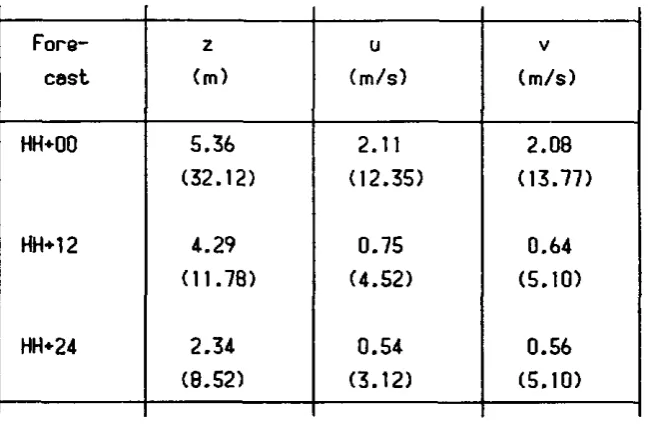
Ia. Rn Equation f o r the Rsymptotic Solution.

To understand how a model responds t o an imposed perturbation, it

is helpful t o study the process o f geostr0~hiC adiustment in a very simple

context. We consider the linearized shallow water equations on an f-plane

We expect t h a t a local disturbance will be dispersed through the radiation o f

gravity waves, leading t o a steady residual flow. However, t h e steady-state o r

time independent f o r m s o f (1)-(3) a r e desenerate in the sense t h a t they are

satisfied by geostrophically balanced flow. They give us no clue regarding

the origin o f such a flow. To find out how a particular initial s t a t e evolves.

we need t o use more information. We may use a physical argument, t h a t each

fluid element retains i t s initial potential vorticity (Rossby. 1930; Obukhov.

1949). Alternatively, we may use a more mathematical approach: the Laplace

transform technique conveniently incorporates the i n ~ t i a l conditions in an

equation f o r the final s t a t e . This l a t t e r approach is used below.

where c a r e t s denote transformed quantities, s is the t r a n s f o r m variable and

zero-subscripts indicate initial values. It is s t r a i g h t f o r w a r d t o derive a single

..

equation f o r 0:

To find an equation f o r the final state. we use a theorem on the asymptotic

behaviour o f Laplace t r a n s f o r m s (Doetsch. 1971, p. 1 4 4 ) :

THEOREM. If t h e limit o f 0 ( t ) , as t tends t o infinity, exists then

_..

Assuming t h a t O ( t ) has such a limit, and denoting it by Om, we take the limit o f (7) t o g e t the equation:

where $, is the initial stream function. This equation gives us the final f o r m o f

the geopotential in t e r m s o f the initial conditions. R similar equation may be

derived f o r the final wind field, or we may simply recall t h a t the asymptotic

s t a t e must be in geostrophic balance, and derive $ - f r o m

Od

lb.

The Importence o f Mass

vs.

Wind Cata.

We now consider the question o f the relative importance o f the

initial perturbations o f the mass and wind fields in determining the final s t a t e .

Assuming t h a t the solution has a wavelike spatial dependence o f the f o r m

where K~ = (k2+12). Since the final s t a t e is geostrophic we also have

em=

S'O,

I- a

The final solutions depend crucially on the size o f the quantity

K

O / f

.

If we define the disturbance length-scale by

L =

l/K,

then the smallness or lar~eness

o f this scale is measured relative t o the Rossby radius o f deformation

L R = j $ / f . Defining t h e r a t i o o f these t w o lengths by a=L/LR we have

L e t us consider the determinat~on o f the disturbance scale. This is influenced

n o t purely by physical extent. but by the size o f the parameter a. In general.

longer wavelengths, higher latitudes and smaller depths all contribute t o larger

values o f a. and thus imply a larue scale disturbance. Contrariwise, small scale

disturbances (small a ) r e s u l t f r o m shorter wavelengths, lower latitudes and

greater depths. We consider now the limits o f (9) f o r large and small a.

1. Large Scale Disturbances (L

w

LR)

In this case a is large and we have,approximately

0

a,

em

'

f'@,

The final fields are determined predominantly by the initial mass field

a,.

The

initial wind field (determined by

Po)

has l i t t l e e f f e c t .

2. Small Scale Disturbances (L c LR)

.

In this case a is small and we have,approximately

0

m

fPo

$',

"

$0

The final fields a r e determined predominantly by the initial wind field

Po.

The

initial mass field is relatively unimportant.

For intermediate scales, L N LR, SO t h a t a l O ( l ) . Both terms in (9) are

important, and t h e initial fields o f both mass and wind are influential in

I c

.

Consequences f o r Data Rssimilation.

The above results have important bearings on the problem o f data

assimilation. The scale o f a perturbation is determined by i t s size relative t o

the deformation radius LR. SO, a perturbation which is large scale in high latitudes may be effectively small scale in the tropics. Similarly, shallow

perturbations (those which project mainly onto modes w i t h small equivalent

depths) will tend t o be large scale, and deep ones small scale. We can also

make the following specific observations:

( i ) A small scale perturbation o f t h e mass field will be radiated away in t h e

f o r m o f gravity waves. and will have l i t t l e e f f e c t on the final s t a t e of t h e

model.

A

large scale mass perturbation will be assimilated more successfully.

(ii) A small scale perturbation o f the wind field will be successfully assimilated.

A large scale wind perturbation will project mainly onto gravity wave

components and will be rapidly dispersed.

(iii) R geostrophically balanced perturbation ( o f any scale) will consist mainly o f

rotational components, and will be assimilated.

The following examples illustrate the problems which may occur.

Suppose we wish t o change the pressure field locally (i.8. on a small scale) t o

deepen a depression; then the wind field must also be changed, if the pressure

alteration is t o survive t h e induction process. Similarly, a modification o f t h e

wind field a t a single level (based on an RIREP, say) must be accompanied by a corresponding alteration o f the mass field, o r it is unlikely t o survive.

Knowledge of t h e winds is crucial f o r small horizontal scales; knowledge o f t h e

mass field is vital f o r shallow systems.

Id. The Rate o f Rdjustment.

We have considered the eventual disturbance resulting f r o m a given

initial perturbation. The more recondite problem o f how t h e disturbance evolves

in time has been avoided (see Cahn, 1945. Obukhov. 1949). However. we can

g e t some idea o f the r a t e a t which the adjustment takes place: a rough

timescale f o r adjustment is given by ( I / v ) , where v is the gravity wave

9 9

length scale L has an adjustment timescale

Thus. the adjustment process is f a s t f o r small scale disturbances and slower

f o r larger scales. It is also f a s t f o r large depths (faster gravity waves) and

slow f o r shallow depths. The r a t e of adjustment does not depend upon the

latitude.

le. Example: an Rxially Symmetric Height Disturbance.

To illustrate the general findings discussed above. we apply equation

(8) t o the simple case of an initial height disturbance with circular symmetry. The following quotation is taken from Charney (1973):

If a stone is thrown into an infinite resting

ocean, the gravitational oscillations engendered w i l l

radiate their energy t o infinity and leave the

ocean Finally undisturbed; if the stone IS thrown

into an infinite rotating ocean, some o f the

energy o f the gravitational oscillations will be

converted by the action OF the Coriolis forces into

rotational motions, and these w i l l persist until

they are dissipated by viscosity.

We consider an axially symmetric initial height perturbation given by

0,

,

r < a

@,

= @,(r) =

{

0

,

r > a The Laplacian in cylindrical coordinates is

where p = r / a and a = a/LR. This is the modified Bessel equation o f order zero. The solution which is bounded a t p = 0 and a t infinity is

C

_c2KO(p)

.

_{p > a}

where

I,

and KO are modified Bessel functions. The constants c, and c2 a r e

found by requiring continuity o f the solution and o f i t s derivative a t p = a. The

final solution is then

@,,,+I-aK,(a)-l,,(p)I

,

p < a

= m

{

(1.10)

Omal,(a)-Ko(p)

,

p > a

The size o f the initial disturbance is measured by a = a/LR, t h a t is, relative t o

the Rossby radius o f deformation. The form o f the final disturbance, plotted

f r o m ( 1 0 ) f o r various values o f a , is shown in Figure 1 . 1 . A large initial

disturbance ( a 3 I ) tends t o persist

-

there is a corresponding geostrophic

circulation around the disturbance. Small initial disturbances do n o t persist, b u t

are radiated away, leaving l i t t l e o r no trace.

-.

-1

If we assume a depth o f 4km and f = 10 s

,

then a = l f o r a disturbance o f radius 2 - 1 0 ~ m . Since t w o megametres is about 1,250 miles, we

may qualify the above quotation:

R stone thrown into en infinite r o t a t i n g ocean will give r i s e t o a persistent disturbance, provided i t

1 -00

,

FINAL FORM OF GEOPOTENTIAL OISTURBAHCE

r / a

7. ASYNOPTIC DATA ASSIMILATION

-

GENERAL CONSIDERATIONS.

78. Introduction.

Continuous data assimilation is, in principle, a unified analysis.

initialization and forecasting technique. The central idea is t o incorporate data

i n t o a prediction model a t i t s time o f validity, w i t h a view t o producing a

sequence o f analyses which are consistent in t h a t they may be i n f e r r e d each

f r o m the other by means o f the model equations. In practice the technique

usually has t h e less ambitious aim t o make good use o f asynoptic data t o

improve f o r e c a s t accuracy. The theory and practice o f f o u r dimensional

assimilation have been reviewed by Bengtsson (1975) and more recently in

(ECMWF, 1905).

With t h e advent o f the new types o f observation, f r o m satellites.

radar networks, etc. the concept o f 'main synoptic hours' f o r analysis has

become less central. It is essential t o be able t o incorporate observations made

a t irregular times. Frequently, useful o r even vital data, valid a f t e r the initial

time o f a forecast, a r e available. For example, f o r a f o r e c a s t s t a r t i n g a t

1430 UTC and based on t h e midday analysis. we may also have local SYNOP data

f o r 1400 and satellite temperature profiles f r o m 1330. and miscellaneous o t h e r

observations may become available during t h e integration. (The operational

ECMWF forecasts based on t h e 1200 analysis don't s t a r t 'till around 2100: yet.

they do n o t use data valid between these times, as f a r as I know).

It would be advantageous t o be able t o data during a

forecast, a t I t s time o f validity. This could be done by a f u l l re-analysis and

re-initialization. However, t h e data may be confined t o a small geographical

region and may be spread over several hours so t h a t constant

plobsl

re-analysis

and re-initialization would be a prohibitively expensive means o f induction. As an

alternative. we could p e r f o r m a analysis, changing the fields in the

vicinity o f the new data a t i t s valid time. There are t w o major difficulties.

111 The analysis problem: how should the fields be changed in the light o f a

point observation: t h a t is, how should we extrapolate the data so t h a t i t

how can we ensure t h a t any imposed changes a r e accepted, so as t o

constructively ~nfluence t h e subsequent evolution o f t h e f l o w ?

7b. Rnalysis. Data Escalation.

The analysis problem, though o f fundamental importance, will n o t be

considered in detail in t h i s r e p o r t . We confine ourselves t o an illustrative

example concerning single-level data. Consider a three-hour forecast, together

w i t h a s e t o f surface pressure observations valid a t t h e same time. Obviously.

we can redefine the vertically integrated mass field. But how do we distribute

t h e changes in the vertical? How should they project onto t h e various vertical

eigenmodes? And how should the wind field be changed? This problem is strongly

under-determined; i t does n o t have a unique answer. We must somehow devise

a means o f optimising the benefits o f whatever choice is made.

Usually. single-level data is extrapolated vertically by the process o f

3-dimensional optimal interpolation, using vertical correlation s t a t i s t i c s . Another

possibility t o incorporate t h i s data in a multi-level model i s by means o f a

t r a d e - o f f between space and time (Charney,

&

el. 1969). Given the h i s t o r y o f

t h e surface fields, t h a t is. a series o f t h e fields a t consecutive analysis

times, it is possible t o use t h e equations o f motion t o deduce compatible field

values a t upper .levels. This can be done by a stepwise procedure, ascending one

vertical level (and losing one time level) per step (Koo. 1959). We will r e f e r t o

t h i s process as escalation. A series o f surface analyses can be escalated

t o provide a f u l l 3-dimensional analysis a t a particular time. J u s t how useful

t h i s process may be in practice appears t o be an open question

( I

am n o t

aware i f i t has ever been t r i e d o u t ) .

We may give a simple example o f t h e t r a d e - o f f between spatial and

temporal data. Consider t h e linear equation

governing small-amplitude long waves in a tank. Normally, we specify initial and