Understanding cumulative risk

PLEASE SCROLL DOWN FOR ARTICLE

On: 17 March 2010

Access details: Access Details: [subscription number 919934172]

Publisher Psychology Press

Informa Ltd Registered in England and Wales Registered Number: 1072954 Registered office: Mortimer House,

37-41 Mortimer Street, London W1T 3JH, UK

The Quarterly Journal of Experimental Psychology

Publication details, including instructions for authors and subscription information: http://www.informaworld.com/smpp/title~content=t716100704

Understanding cumulative risk

Rachel McCloy a; Ruth M. J. Byrne b; Philip N. Johnson-Laird c

a University of Reading, Reading, UK b Trinity College Dublin, University of Dublin, Dublin, Ireland c

Princeton University, Princeton, NJ, USA

First published on: 17 March 2010

To cite this Article McCloy, Rachel, Byrne, Ruth M. J. and Johnson-Laird, Philip N.(2010) 'Understanding cumulative risk', The Quarterly Journal of Experimental Psychology, 63: 3, 499 — 515, First published on: 17 March 2010 (iFirst)

To link to this Article: DOI: 10.1080/17470210903024784 URL: http://dx.doi.org/10.1080/17470210903024784

Full terms and conditions of use: http://www.informaworld.com/terms-and-conditions-of-access.pdf This article may be used for research, teaching and private study purposes. Any substantial or systematic reproduction, re-distribution, re-selling, loan or sub-licensing, systematic supply or distribution in any form to anyone is expressly forbidden.

Understanding cumulative risk

Rachel McCloy University of Reading, Reading, UK

Ruth M. J. Byrne

Trinity College Dublin, University of Dublin, Dublin, Ireland

Philip N. Johnson-Laird Princeton University, Princeton, NJ, USA

This paper summarizes the theory of simple cumulative risks—for example, the risk of food poisoning from the consumption of a series of portions of tainted food. Problems concerning such risks are extraordinarily difficult for naı¨ve individuals, and the paper explains the reasons for this difficulty. It describes how naı¨ve individuals usually attempt to estimate cumulative risks, and it outlines a computer program that models these methods. This account predicts that estimates can be improved if problems of cumulative risk are framed so that individuals can focus on the appropriate subset of cases. The paper reports two experiments that corroborated this prediction. They also showed that whether problems are stated in terms of frequencies (80 out of 100 people got food poisoning) or in terms of percentages (80% of people got food poisoning) did not reliably affect accuracy.

Keywords: Cumulative risk; Probability judgment; Mental models; Frequencies.

Suppose you are trying to decide between two drugs to reduce blood pressure, and both have a harmful side effect. The risk of harm from Drug A is 1% over a year—that is, on average only 1 person out of every 100 using the drug for a year should suffer the side effect. The risk of harm from Drug B is 3% over a year. The difference

may seem negligible. But the cumulative risks of experiencing the side effect at least once over 10 years differ markedly for the two drugs: 10% for Drug A and 26% for Drug B. A small difference in short-term risk can become significant in the long term (Slovic, Fischhoff, & Lichtenstein, 1982).

Correspondence should be addressed to Rachel McCloy, School of Psychology, University of Reading, Harry Pitt Building, Earley Gate, Reading RG6 6AL, UK. E-mail: [email protected]

This research was carried out while the first author was a postdoctoral fellow at Trinity College, University of Dublin, funded by a Medical Research Council grant to Ruth Byrne. We thank Dai Rees and Ian Robertson for their support of the research and for helpful comments at various meetings on cumulative risk. The research was also funded in part by the Dublin University Arts and Social Sciences Benefactions Fund and by a grant to Phil Johnson-Laird from the National Science Foundation (BCS 0076287) to investigate strategies in reasoning. We thank Michele Cowley for her help with Experiment 2. We are grateful to Vittorio Girotto, David Green, Baruch Fischhoff, David Klahr, Alessandra Tasso, Paul Slovic, and Clare Walsh, for helpful comments especially during the meeting on “Mental Models and Understanding Science” held in Dublin in 2001, funded by the European Science Foundation, and Phil Beaman for comments on earlier versions of the paper.

#_{2009 The Experimental Psychology Society}

499

Now suppose you are given a drug that has a risk of a harmful side effect of 5% in a year. What are the chances that you will not experi-ence the harmful side effect if you take the drug for a period of five years? The question calls for an estimate of a cumulative risk (Slovic, 2000). The answer is that there is a 78% chance that the harmful side effect will not occur over five years. Most people find such pro-blems very difficult. In one study, only 1 or 2 people in every 100 got the right answer (see Doyle, 1997). Consider the question from another angle: What are the chances that you

will experience the harmful side effect at least once in the five-year period? The answer is 22%, but again very few people are correct (Doyle, 1997; Shaklee & Fischhoff, 1990; Svenson, 1984, 1985). Cumulative-risk judge-ments are hard (Kahneman, Slovic, & Tversky, 1982). Yet to make good decisions, people need to be able to understand the risks that exist and how they accumulate over time. Our goal in this paper is to establish why cumulative risk is so difficult for people to understand and to devise ways to help individuals to arrive at more accurate assessments of cumulative risk. We report the results of two experiments designed to improve understanding of cumulative risks, and we describe a computer program that simu-lates the strategies that people use to estimate cumulative risks.

Cumulative risk

How risk accumulates depends on its nature (Bedford & Cooke, 2001; Diamond, 1990). Consider a simple illustration. You take a drug over a sequence of trials, and on each trial there is a certain fixed probability of a harmful outcome. For simplicity, we assume that the prob-ability of the harmful outcome is 1/3 on each occasion that you take the drug. What is the prob-ability that exactly two harmful outcomes occur in a series of three trials? On the assumption that the chances of the harmful outcome areindependent— that is, that what happens on one trial has no effect on any other trial—the answer is given by the

binomial formula:

Probability (exactlymharmful outcomes inntrials)

¼(nCm)pm(1p)n

m

wherenis the number of trials,mis the number of harmful outcomes, (nCm) is the number of

differ-ent ways (combinations) of drawingm cases out of nevents¼_n!/_m!(n – m)!, and p is the prob-ability of the harmful outcome. Hence:

(3C2)¼3!=2!(32)!¼3

pm_¼(1=3)2 ¼1=9

(1p)nm¼(11=3)1¼2=3

and the required probability, which is the product of these three numbers, is (3)(1/9)(2/3)¼2/9.

Naı¨ve individuals—that is, individuals who have not mastered the probability calculus—do not know the binomial formula and certainly do not use it to compute cumulative risks. But, there are two special cases that they might be able to compute by other means, and these two cases are highly pertinent to risks in daily life. The first case concerns theconjunctiveprobability that no bad outcomes occur in a series of trials— that is, the bad outcome does not occur on the first trial and it does not occur on the second trialand. . .it does not occur on the nth trial. In this conjunctive case,m¼0, and so the binomial formula above simplifies to:

Probability (exactly 0 bad outcomes inntrials)

¼(1p)n

In our example of the drug, the probability of no bad outcomes in three trials is (1 – 1/3)3¼8/27. The second special case of the binomial formula concerns thedisjunctiveprobability of at least one bad outcome in a series of n trials—that is, the bad outcome occurs on the first trial orit occurs on the second trialor. . .it occurs on thenth trial, where the disjunction allows for the bad outcome on any or every trial. In this disjunctive case, the

probability can be obtained by summing the exact probabilities according to the binomial formula for 1, 2, . . . and so on, up to m bad outcomes. But, there is a simpler solution:

Probability (at least 1 bad outcome inntrials)

¼1 probability (exactly 0 bad outcomes in ntrials)

Hence, the disjunctive probability is: 1 – the conjunctive probability. In the drug example, the probability of at least one bad outcome in three trials is (1 – 8/27)¼19/27. Naı¨ve individuals are, however, unlikely to know even the simpler for-mulae for these two special cases of conjunctive and disjunctive cumulative probabilities.

Samuel Pepys, the great diarist, wrote a letter to Newton asking whether the following three prob-abilities were the same:

the probability of getting at least 1 six in throwing 6 dice,

the probability of getting at least 2 sixes in throwing 12 dice,

and the probability of getting at least 3 sixes in throwing 18 dice.

The reader is invited to think about this problem in cumulative probabilities and then to use the binomial formula to arrive at Newton’s reply. (For those readers who are disinclined to do the calculations, the answers can be found at the end of the paper.) If intelligent individuals such as Pepys do not use the binomial formula, or its simpler special cases, how do people understand conjunctive and disjunctive cumulative risks?

Naı¨ve cumulative-risk judgements

The evidence so far on naı¨ve individuals’ perform-ance on simple cumulative-risk judgements shows that people make substantial and systematic errors in judging cumulative risk (Doyle, 1997; Knauper, Kornik, Atkinson, Guberman, & Aydin, 2005; Shaklee & Fischhoff, 1990). Shaklee and

Fischhoff (1990) found that, when given conjunc-tive problems about the chances of avoiding pregnancy using different contraceptives, only half of their participants realized that this probability would consistently decrease when looked at cumu-latively. Other participants assumed that the probability of avoiding pregnancy would remain constant, increase, or vary nonmonotonically. Those participants who realized that the prob-ability would decrease across time often underesti-mated the rate of the decrease. They also failed to notice how a small difference in short-term risk could translate into a large difference over time.

Doyle (1997) studied both simple conjunctive and simple disjunctive cumulative-risk judge-ments. In four studies, he looked both at the con-traceptive domain used by Shaklee and Fischhoff, and also at a novel domain (natural disasters). He presented his participants with scenarios such as:

Suppose that the probability that your house will be hit one or more times by the natural hazard during an exposure period of one year is .005. That is, if 1,000 homes like yours were exposed to the natural hazard for one year, 5 of the homes would be damaged. Please estimate the probability that your homewould avoid being hit by the natural hazard (conjunctive)/_{would be hit at least}

once by the natural hazard (disjunctive) if exposed to the hazard for a period of. . ..

Doyle then asked his participants to make esti-mates of the probability for a range of time periods: 1 month, 1 year, 5 years, 10 years, 25 years, and 50 years for natural hazards (1 month, 1 year, 5 years, 10 years, 15 years, and 25 years for contraceptives). Doyle also varied the single-year probability across scenarios. Like Shaklee and Fischhoff (1990), he found that a substantial proportion of participants failed to realize that the probability would decrease monotonically over time for con-junctive cumulative-probability judgements (50% for the contraceptive domain, 25% for the natural hazards domain). Of those participants, most either assumed that the probability would remain

constant over time (i.e., the single-year probability at all time periods) or that it would increase over time. For participants who did show a monotoni-cally decreasing function, though the majority used some kind of analytic strategy to compute their responses, only 2 participants used the normatively correct strategy to arrive at their answers. The most common analytic strategies used were an anchoring and subtraction strategy (where participants started with the single-year probability and systematically subtracted a certain amount each time to arrive at their judgements) and a multiplicative strategy (where participants multiply the probability of experiencing the hazard in a single year by the number of years and subtract this from 1), both of which drop more sharply over time than the normatively correct answers. Few participants employed an intuitive or guessing strategy, suggesting that participants generally found the problems to be tractable, but that they misrepresented them or employed an inappropriate strategy.

For judgements of disjunctive cumulative probabilities, Doyle found a similar pattern. Some participants failed to realize that, for these judgements, the probability should increase mono-tonically over time (28% for contraceptives, 16% for natural hazards). Most participants showed some form of analytic strategy, although none used the normatively correct one. The most popular strategy used on disjunctive cumulative-probability problems was a multiplicative one (where participants multiplied the probability of experiencing the event by the number of years). This strategy results in probability estimates that increase more quickly than the normatively correct answers, and it led some participants to make probability estimates of greater than 1 (with others abandoning the strategy when it reached this point). The above evidence suggests that people are poor at making even the simplest cumulative-probability judgements (Doyle, 1997; Shaklee & Fischhoff, 1990), never mind when they are faced with judgements where the single-year probability varies over time (Svenson, 1984, 1985). How can we help people better understand how risk accumulates over time?

Improving risk judgements

Although little work has been carried out specifi-cally on improving people’s understanding of cumulative probabilities, research into people’s performance on other kinds of probability judge-ment problems may be informative. Another class of probability judgement problems on which people traditionally perform poorly are Bayesian conditional probability judgements, such as:

The probability that a woman between 40 and 50 years has breast cancer is 0.8%. If a woman has breast cancer, the probability that this will be successfully detected by a mammogram is 90%. If a woman does not have breast cancer there is a 7% probability of a false-positive result on the mammo-gram. A woman (age 45) has just tested positive on a mammogram; what is the prob-ability that she actually has breast cancer?

Naı¨ve individuals do not use Bayes’s theorem in responding to problems such as this one and rarely arrive at normatively correct solutions (Casscells, Schoenberger, & Grayboys, 1978; Eddy, 1982; Hammerton, 1973). They tend to underweight information on the base rate (here 0.8%, e.g., Kahneman & Tversky, 1982; cf. Koehler, 1996), and they tend to confuse the conditional probability with its converse ( Johnson-Laird, Legrenzi, Girotto, Sonino-Legrenzi, & Caverni, 1999).

One view of these problems is that errors arise because the problems are stated in terms of prob-abilities rather than in terms of frequencies of the sort observed in daily life—that is, “natural” samples (Cosmides & Tooby, 1996; Gigerenzer & Hoffrage, 1995). According to this frequentist

view, probabilities concern repeated events, and those assigned to unique events in nonextensional problems are meaningless. An event such as World War III either happens or does not happen, and it does not happen with a probability of .85 (Cosmides & Tooby, 1996). Gigerenzer and Hoffrage (1995) showed that if conditional prob-ability problems such as the one above were

presented in terms of frequencies as opposed to probabilities, then participants were more likely to arrive at the correct answer. This result suggests one way in which we might be able to improve individuals’ judgements of cumulative probability: We should present the problems in terms of natural frequencies rather than in terms of probabilities.

However, there are another group of studies that suggest that it is not the numbers (frequencies or probabilities) in problems that are important. These studies suggest instead that how infor-mation is structured is the key to improving performance (Evans, Handley, Perham, Over, & Thompson, 2000; Girotto & Gonzalez, 2001; Johnson-Laird et al., 1999; Macchi, 2000; Sloman, Over, Slovak, & Stibel, 2003). Individuals make better judgements of conditional probabilities when problems are presented in this way (Girotto & Gonzalez, 2001, p. 253):

A person who was tested has 4 chances out of 100 of having the infection. 3 of the 4 chances of having the infection were associ-ated with a positive reaction to the test. 12 of the remaining 96 chances of not having the infection were also associated with a positive reaction to the test. Imagine that Pierre is tested now. Out of a total of 100 chances, Pierre has ___ chances of having a positive reaction, ___ of which will be associated with having the infection.

These problems used information on chances that refer to single-event probabilities but can readily be structured in the same manner as “natural” frequencies (see also Girotto & Gonzalez, 2002). And they call for separate estimates of the denomi-nator and the numerator of the conditional probability. Girotto and Gonzalez (2001) also showed that frequency versions of these problems that do not have this useful structure lead to poor performance on the task.

One theory that provides a clear account of how this restructuring of information may help to improve people’s understanding of conditional probabilities is the mental model theory of naı¨ve probability judgement (Johnson-Laird et al.,

1999). We describe some of the relevant aspects of this theory below and consider how it might extend to the consideration of cumulative-probability judgements.

Models and extensional probabilities

The probability calculus embodies several self-evident principles—notably, the extensional

notion that the probability of an event equals the sum of the probabilities of the mutually exclusive ways in which the event can occur. The probability calculus is therefore a normative theory of exten-sional reasoning about probabilities. This way of reasoning aims to be deductive—that is, if no errors occur, then conclusions must be true given that the premises are true. It can be contrasted with nonextensionalreasoning about probabilities, which relies on relevant evidence or a relevant index. Nonextensional reasoning is inductive— that is, its conclusions could be false even if the premises are true. It occurs, for instance, when individuals infer that because an exemplar is typical of a category, it is very probably a member of the category. Kahneman and Tversky in their seminal studies have shown that nonexten-sional reasoning depends on a variety of such heur-istics (see, e.g., Tversky & Kahneman, 1983).

Extensional reasoning about probabilities depends on thinking about the possibilities in which an outcome occurs, and reasoners use the probabilities of these possibilities to infer the probability of the outcome. People think about possibilities to make various sorts of deductions (e.g., Johnson-Laird & Byrne, 1991, 2002), and a theory of extensional reasoning about probabil-ities follows from the assumption that individuals represent possibilities in separate mental models (Johnson-Laird et al., 1999). This theory suggests that each model represents only what is true in the relevant possibility (the “principle of truth”). In default of information to the contrary, individuals assume that each model of a possibility is equi-probable (the “principle of equiprobability”). People compute the probability of an event by assessing the proportion of models in which the event occurs (the “principle of proportionality”).

This theory was corroborated by various exper-iments ( Johnson-Laird et al., 1999) that tested the following prediction: Bayesian inference of posterior conditional probabilities either about unique events or about repeated events should be easier when models directly represent probabilities according to the basic principles of the theory.

Consider the following well-structured Bayesian problem, for example:

The chances that Pat has the disease are 4 out of 10. If she has the disease, then the chances are 3 out of 4 that she has the symptom. If she does not have the disease, then the chances are 2 out of 6 that she has the symptom. If Pat has the symptom, what are the chances that Pat has the disease?

Individuals can build a set of equiprobable models of the possibilities, or they can build models tagged with their appropriate numerical frequencies:

Frequencies

disease symptom 3

disease :symptom 1

:disease symptom 2

. . . 4

where the ellipsis represents the cases where Pat has neither the disease nor the symptom (as people may not fully represent this possibility, in line with the theory’s principle of truth). The set of models establishes that the probability that Pat has the symptom is 5 out of 10 (the combined frequency of lines 1 and 3 above), and that the probability that Pat has the disease given the pres-ence of the symptom is 3 out of 5. The posterior probability can therefore be computed without having to use Bayes’s theorem. A simpler pro-cedure suffices based on the use of subsets of models ( Johnson-Laird et al., 1999):

Granted equiprobability, a conditional prob-ability, p(AjB), depends on the subset of B that is A, and the proportionality of A to B yields the numerical value. Otherwise, if the models are tagged with their absolute fre-quencies (or chances), then the conditional

probability equals the frequency (chance) of the model of A and B divided by the sum of all the frequencies (chances) of models containingB.

Inferences about posterior probabilities should be easier when the statement of the problem makes it simple to envisage the required subset, and the mental arithmetic is easy, regardless of whether the numbers concern the chances of unique events or the frequencies of repeated events (Johnson-Laird et al., 1999). One advantage of this theory is that it can explain the results of Gigerenzer and Hoffrage’s (1995) studies without recourse to a specific adaptation for dealing with so-called natural frequencies. Many empirical results are compatible this account (see, e.g., Evans et al., 2000; Girotto & Gonzalez, 2001; Macchi, 1995; but cf. Girotto & Gonzalez, 2002; Hoffrage, Gigerenzer, Krauss, & Martingnon, 2002). Errors in probabilistic reasoning result when the mental models that people construct and the real alternatives relevant to the problem do not match (e.g., in the Monty Hall problem; see Johnson-Laird et al., 1999).

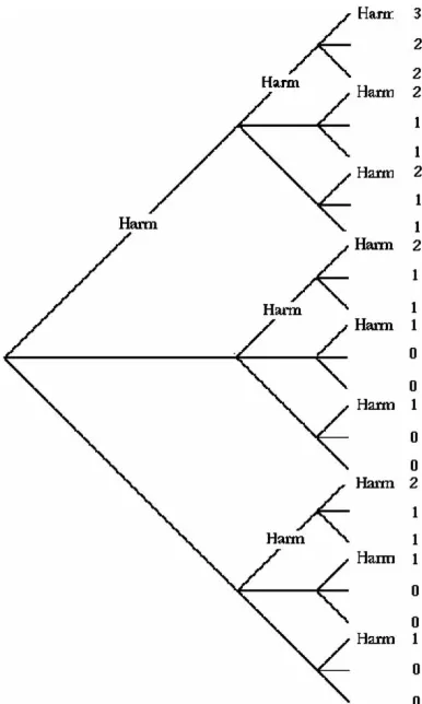
The mental model theory extends naturally to the computation of cumulative risk. Figure 1 pre-sents a diagram corresponding to the partition of events in which there are three trials, and on each of them, as in the example above about the drug, the probability of a harmful outcome is 1/

3. Naı¨ve individuals may be able to construct such a diagram in which each complete branch denotes, in effect, an equiprobable sequence of three trials. Each node corresponds to a trial, and the three lines emanating from each node show that the chance of a harm is 1/3—that is, only one of the three lines is labelled “harm”. The right-hand side of the diagram shows the number of times “harm” occurs in each sequence of three trials. It is a simple matter to add up the numbers required for the conjunctive probability: There is no harmful outcome on any of the three trials for 8 out of the 27 possible sequences. Likewise, the disjunctive probability of at least one harmful outcome in three trials is 19 out of the 27 possible sequences of trials.

The partition in Figure 1 represents the possible sequences of three independent trials. Suppose that we wanted the figure to represent three shots in a game of Russian roulette in which there were bullets in two of the six chambers in the revolver. The trials are no longer indepen-dent: If a harmful event occurs, then death follows, and so there are no further trials. “Harm” on an edge of the graph is terminal in the other sense of the word as well—that is, the graph ends at this point, because the harmful outcome can occur to a player only once. What is the probability of a conjunctive sequence—that is, one in which the harmful outcome does not

occur in a series of three trials? Inspection of Figure 1 but with all edges terminating with the label “harm” shows that there are now only 15 possible sequences of trials: A total of 7 terminate with the ultimate harmful event, and 8 terminate without the harmful event. Hence, the probability of death is 7/15 and of continuing life is 8/15.

Consider the risk of pregnancy with a certain method of contraception. If the risk of pregnancy is stated over a period of time, such as a year, then it can be treated as an independent risk over lengthy periods of time. Strictly speaking, however, the risk should be stated, not in relation to a certain period of time—any method will be risk free if a woman does not have sexual inter-course during that period of time—but rather it should be stated as a function of the number of occurrences of intercourse. However, when a woman becomes pregnant, there is no further risk of pregnancy for some time. In terms of the sort of partition illustrated in Figure 1, when a woman becomes pregnant she ceases to engage in further trials at which she is at risk, not perma-nently as in Russian roulette, but until she is able to conceive again. A further source of complexity is that the risk of pregnancy may change over

time depending on hormonal effects from certain methods of contraception. The moral is that cumulative risk over a series of dependent events can be very complicated. For this reason, our investigation focuses on independent events, especially as people have been shown still to have problems with even the most straightforward kind of cumulative risk (e.g., Doyle, 1997).

According to the model theory, a way to help naı¨ve individuals to make cumulative estimates is to step them through each trial in an iterative way, especially if the iteration focuses on the relevant subsets. Given, say, the partition in Figure 1, individuals should be asked to make the conjunctive estimate in the following sequence of iterated estimates:

If 27 people take the drug with a probability of a harmful side effect of 1/3 on each trial, how many are likely not to suffer the side effect on the first trial?

Figure 1.Diagram illustrating a series of three trials on which the probability of harm on any trial is 1/3. The right-hand column sums the number of harmful events in each sequence of trials.

[Answer: 18 out of the 27]

How many of these individuals in turn are likely not to suffer the side effect on the second trial too?

[Answer: 12 out of the 18]

And how many of these in turn are likely not to suffer the side effect on the third trial?

[Answer: 8 out of 12]

Each estimate in the iteration should be rela-tively easy to make.

The theory suggests that differences between estimates from frequencies and from probabilities are likely to occur only when they are confounded with the difficulty of the corresponding mental arithmetic, or with the ease of recovering the per-tinent subset. Evidence has corroborated this prediction for probability estimates (see, e.g., Girotto & Gonzalez, 2001). But, in order to test the frequentist prediction for cumulative risk, our first study examined the difference between problems based on probabilities and those based on frequencies. It also examined the difference between problems in which the relevant subset was made salient and problems in which it was not.

Strategies

As our interest is in helping people to under-stand cumulative risks, we are concerned not only with the estimates that people make when faced with cumulative-risk problems, but also with the strategies that they employ in calculat-ing cumulative risks. Doyle (1997) highlighted a number of erroneous strategies employed by his participants. For conjunctive cumulative-risk problems two of the most common strategies that people use areanchoring and subtraction, and

constant (Doyle, 1997). For the anchoring and subtraction strategy, participants start with the single-event probability and subtract a particular percentage for each subsequent event, and for the constant strategy, participants assume that the cumulative probability remains constant and equal to the single-event probability over the

duration of the time period at question. Doyle’s participants produced the same (constant) or similar (anchoring and addition) strategies for disjunctive cumulative-risk problems. We predict that, if the relevant subset is made easier to access, participants will be less likely to use such erroneous strategies.

EXPERIMENT 1: CONJUNCTIVE AND

DISJUNCTIVE CUMULATIVE RISK

A standard version of a conjunctive risk problem is shown here:

A. In a remote village there is an outbreak of an infection, which causes damage to the retina of the eye, once every year. In any one year, the probability of a person in the village becoming ill with the infection is 30%. That is, a person from the village has a 70% probability of not suffering from the infection over the course of a year. What is the probability that a person living in the village for a period of three years will not suffer from the infection?

The same premises can be used for a disjunctive problem, which replaces the final question with:

What is the probability that a person living in the village for a period of three years will become ill with the infection at least once?

Naı¨ve participants find these problems very dif-ficult (Doyle, 1997). Hence, the present exper-iment called for the participants to make iterative estimates before they made cumulative estimates, the arithmetic was always with whole numbers, and all estimates were of separate values for the numerator and the denominator. On each trial, the participants accordingly answered five ques-tions illustrated here in the version used for the eye infection problem:

1. Suppose that 1,000 people live in the village for one year—how many of these people do you think would not suffer from

the infection at all that year? ___ out of ___. [One-year conjunctive risk]

2. Now suppose that these 1,000 people con-tinued to live in the village for asecond year—

how many of these people do you think would not suffer from the infection at all over the two years (bearing in mind that there is a 70% probability of not suffering from the infection)? ___ out of ___. [Two-year conjunctive risk]

3. Now suppose that these 1,000 people live in the village for athird year—how many of these people do you think would not suffer from the infection at all over the three years (bearing in mind that there is a 70% probability of not suffering from the infec-tion)? ___ out of ___. [Three-year conjunc-tive risk]

4. So, over the three years, how many people out of the original 1,000 will not have suffered from the infection at all? ___ out of 1,000. [Overall conjunctive risk]

5. And how many people out of the original 1,000 will have become ill with the infection at least once during the three years? ___ out of 1,000. [Overall disjunctive risk]

The aim of the experiment was to examine two ways that might enable individuals to improve their judgements of cumulative risk. First, accord-ing to the model theory, the presentation of pro-blems in a way that highlights the pertinent subset should improve performance. The exper-iment therefore compared the nonsubset version of a problem shown above with a subset version in which the subset was made salient. These pro-blems were constructed by replacing the questions 2 and 3 above with questions that focused on the relevant subset of people:

20_{. Now suppose that those people who did}

not suffer from the infection at all in the first year continued to live in the village for a second year—how many of those people who did not suffer from the infection during the first year do you think would

also not suffer from the infection at all during the second year (bearing in mind that there is a 70% probability of not suffer-ing from the infection)? ___ out of ___.

30_{. Now suppose that those people who did}

not suffer from the infection at all during the second year continued to live in the village for athird year—how many of those people who did not suffer from the infection during the second year do you think would also not suffer from the infection at all during the third year (bearing in mind that there is a 70% probability of not suffering from the infection)? ___ out of ___.

Second, according to frequentist accounts (e.g., Gigerenzer & Hoffrage, 1995), the statement of a problem in terms of frequencies should improve performance. The experiment therefore compared the probabilityversion of a problem, as above, with a frequency version. The initial pre-mises for the eye disease problem were accordingly as follows:

A0_{. In a remote village there is an outbreak of}

an infection, which causes damage to the retina of the eye, once every year. In any one year, 30 out of every 100 people become ill with the infection. That is, 70 out of every 100 people do not suffer from the infection over the course of a year.

Likewise, in Questions 2 and 3 the parenthetical reminder was phrased in frequencies: “bearing in mind that 70 out of every 100 people do not suffer from the infection”. If the model theory is correct, then this manipulation is unlikely to have as large an effect as the subset manipulation.

Method

Design

There were four separate groups of participants, which each tackled three problems. The four groups were defined in terms of whether the three problems were in a subset version or nonsub-set version and whether they were stated in terms of frequencies or probabilities. The three problems

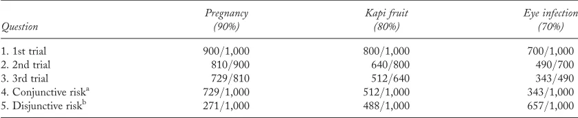
in each group differed in content and in the prob-ability of no harmful outcome (90%, 80%, and 70%). The three problems concerned respectively pregnancy, kapi fruit, and eye infection, and their premises are stated in the Appendix. Table 1 states their correct answers. Each participant received the problems in a different random order.

Participants

The participants were from Trinity College Dublin (30 undergraduates and 7 others) and took part in the experiment at the end of a practical class. They were assigned at random to one of the four groups, subset frequency (n¼9), subset prob-ability (n¼10), nonsubset frequency (n¼9), and nonsubset probability (n¼9).

Procedure

The participants were given a five-page booklet, which consisted of an instruction page, three pro-blems on separate pages, and a final debriefing page. The instructions stated that they were to read through the problems carefully, to write down their calculations in the rough-work spaces provided, and to answer the questions and the pro-blems in the order in which they were given. They were required to use paper and pencil to arrive at their answers, and calculators were not provided. They were allowed as much time as they needed

to complete the problems, and they took about 15 minutes to complete all three.

Results

The participants had to make 8 separate numerical estimates for each problem (the numerator and denominator for Questions 1, 2, and 3, and the conjunctive and disjunctive estimates in Questions 4 and 5). Across the three problems, therefore, each participant made a total of 24 esti-mates (the 8 estiesti-mates for each of three problems). The mean numbers of correct answers (out of 24) were as follows:1

Subset frequency group: 22.3

Subset probability group: 21.7

Nonsubset frequency group: 14.2

Nonsubset probability group: 16.7.

The participants in the subset groups (mean 22.0) were significantly more accurate than those in the nonsubset groups (mean 15.44; Mann–Whitney

U¼70.5,z¼3.12,p,.001). The participants in the frequency groups were not significantly more accurate (mean 18.28) than those in the probability groups (mean 19.32; Mann–Whitney U¼161,

z¼0.31, p,.4).Within the nonsubset groups, there was no reliable difference between the fre-quency and the probability groups (mean 14.22 vs.

Table 1.The correct answers for the subset versions of three problems in Experiment 1

Question

Pregnancy (90%)

Kapi fruit (80%)

Eye infection (70%)

1. 1st trial 900/1,000 800/1,000 700/1,000

2. 2nd trial 810/900 640/800 490/700

3. 3rd trial 729/810 512/640 343/490

4. Conjunctive riska _{729/1,000 512/1,000 343/1,000}

5. Disjunctive riskb _{271/1,000 488/1,000 657/1,000}

Note:Percentages show the probability of no harmful outcome for each problem. The same answers are accurate for both probability and frequency versions. The subset and nonsubset problems have the same answers for Questions 1, 4, and 5 and differ only in the denominator for Questions 2 and 3 (e.g., the nonsubset answer to Question 2 for the pregnancy content is 810/1,000).

a

No harmful outcome over 3 years.bAt least one harmful outcome over 3 years.

1_{The pattern of results is the same if we consider only correct numerators.}

mean 16.67; Mann–WhitneyU¼30.5,z¼0.91,

p,.2). Likewise, within the subset groups, there was no significant difference between the frequency and the probability groups (mean 22.33 vs. mean 21.7; Mann–WhitneyU¼38.5,z¼0.56,p,.3). In their estimates of the conjunctive and disjunctive probabilities (Questions 4 and 5), the participants in the subset groups were more accu-rate (conjunctive mean¼2.32 out of 3, disjunctive mean¼2.12) than those in the nonsubset groups (conjunctive mean¼1.28, disjunctive mean¼

1.06; conjunctive Mann –Whitney U¼110,

z¼2.01, p,.02; disjunctive Mann –Whitney

U¼101.5, z¼2.24, p,.01). There was no reliable difference in accuracy between the fre-quency and probability groups (frefre-quency conjunc-tive mean¼1.56, frequency disjunctive mean¼

1.39; probability conjunctive mean¼2.05, prob-ability disjunctive mean¼1.79; conjunctive Mann – Whitney U¼142, z¼0.957, p,.19; disjunctive Mann –Whitney U¼140.5, z¼

0.984,p,.18). Frequency groups performed mar-ginally worse than probability groups in the non-subset condition (conjunctive mean 0.67 vs. mean 1.89, Mann – Whitney U¼23.5, z¼1.71,

p,.08, two-tailed; disjunctive mean 0.67 vs. mean 1.44, Mann –WhitneyU¼28.0, z¼1.29,

p,.17, two-tailed), but not in the subset con-dition (conjunctive mean 2.44 vs. mean 2.20, Mann – Whitney U¼37.5, z¼0.69, p,.32, two-tailed; disjunctive mean 2.11 vs. mean 2.10, Mann – Whitney U¼44.5, z¼– 0.04, p,.52, two-tailed). Overall, participants were more accu-rate on the conjunctive question (mean 1.81) than on the disjunctive question (mean 1.59) but this difference was only marginally significant (Wilcoxon,z¼2.06,p,.07).

Strategies

We were able to discern from the participants’ rough work and responses the strategies that they had used on 98% of the trials. The majority of par-ticipants showed some rough work in addition to the production of answers, which indicates that they were engaging with the task and endeavouring to arrive at a correct solution. Participants used three main strategies. The most frequent strategy

was to use the appropriate subset to calculate the correct answers. They used this strategy on 65% of trials, but made some arithmetical errors (54% correct responses, 11% arithmetical errors). The participants tried to work out the proportion of people who had avoided the harmful outcome on the first occasion, those who continued to avoid it on the second occasion, and so on. This strategy accounted for the correct answers in both con-ditions. A second strategy (19% of trials) was to assume erroneously that the number of people avoiding harm decreased by a constant number on each occasion (cf., anchoring and subtraction; Doyle, 1997). In the eye infection problem, for example, these participants assumed that because the number of people avoiding infection decreased by 300 in the first year, it would continue to decrease by 300 in each subsequent year. The third strategy (14% of trials) was to assume that the number of people avoiding the harmful outcome remained constant over the course of the three occasions (cf., constant; Doyle, 1997). In the eye infection problem, for example, they believed that 700 out of 1,000 people would have avoided being infected at all not only after the first year, but also after subsequent years.

We predicted that participants in the subset groups should be more likely to use the subset strategy than those in the nonsubset groups. Table 2 shows the number of participants who used the subset strategy on two or more problems and the number who used it on fewer than two problems. A Fisher – Yates exact test showed that participants in the subset groups were significantly more likely to use the strategy than those in the nonsubset groups (p,.002).

Table 2.The number of participants using the subset strategy in the subset and nonsubset groups in Experiment 1

Subset strategy

Group n

On 2 or more problems

On fewer than 2 problems

Subset 19 17 2

Nonsubset 18 7 11

Note:Participants include those who made arithmetical errors.

Discussion

It is possible to help individuals to make accurate estimates of cumulative risk. In all the groups in the experiment, performance was much better than that in previous studies. Hence, iterative esti-mates, the separation of numerator and denomi-nator, and the use of simple arithmetic are all likely to improve estimates. This overall improve-ment is all the more surprising, given that in this experiment we employed a strict (exact) criterion for correct answers, unlike the criteria used in some previous studies. The experiment showed, however, that when a problem is framed in terms of the relevant subset, then performance is reliably enhanced in comparison with groups who received problems framed otherwise. The reason for this improvement was probably because when the subset is salient, the participants used a strategy based on its use in estimates. The improvement occurred whether or not problems were stated in terms of frequencies or probabilities. Indeed, contrary to frequentist views, this variable had no reliable effect on performance, though there was a tendency, albeit not significant, for fre-quencies to impair performance with nonsubset problems.

There was little difference between the estimates of conjunctive and disjunctive risk. Participants appear to have based their answers to the disjunctive question on a simple subtraction from the conjunctive answer. Indeed, the partici-pants’ strategies show that differences in accuracy between the conjunctive and disjunctive estimates arose from errors in subtraction in making the dis-junctive estimate. Our next experiment examines disjunctive cumulative risk in more depth.

EXPERIMENT 2: DISJUNCTIVE

CUMULATIVE RISK

The second experiment aimed to show that the subset principle can also be applied when people are focused on estimates of disjunctive risk rather than conjunctive risk. Consider the kapi fruit problem used in Experiment 1:

Kapi fruit is a popular delicacy in part of the world. Even when correctly prepared kapi fruit may still contain some toxins, and there is a 20% probability that a person eating a portion of kapi fruit will suffer from severe stomach pains and develop some liver damage. That is, there is an 80% probability that a person eating a portion of kapi fruit will suffer no ill effects.

In Experiment 1, people were asked a conjunctive question at each stage about the numbers of people avoiding harm. In contrast, in our second exper-iment the iterative questions concerned disjunctive estimates, which are shown here with their correct answers:

1. Suppose that 1,000 people each eat asingle portion of kapi fruit. How many of these people do you believe will suffer from severe stomach pains? [200 out of 1,000].

2. Now suppose that these 1,000 people each eat asecond portionof kapi fruit—how many additional people do you believe will suffer severe stomach pains for the first time from eating a second portion (bearing in mind that there is a 20% probability of suffering from severe stomach pains)? [160 out of 1,000].

3. Now suppose that these 1,000 people each eat athird portionof kapi fruit—how many additional people do you believe will suffer severe stomach pains for the first time from eating a third portion (bearing in mind that there is a 20% probability of suffering from severe stomach pains)? [128 out of 1,000].

The participants were then given the cumulative

disjunctivequestion:

4. So, out of the original 1,000 people who ate kapi fruit, how many will have become ill at least once over the three portions? [488 out of 1,000].

and finally the (complementary) cumulative con-junctivequestion:

5. And how many out of the original 1,000 will not have suffered any ill effects? [512 out of 1,000].

For the subset version of the problems, the questions again focused participants on the relevant subset:

20_{. Now suppose that those people who}

suf-fered no ill effects from eating the first portion of kapi fruit each eat a second portion of kapi fruit – How many of these people who did not suffer any ill effects from the first portion do you believe will suffer severe stomach pains from eating the second portion (bearing in mind that there is a 20% probability of suffering from severe stomach pains)? [160 out of 800].

Question 3 was modified in the same way, and its correct answer was 128 out of 640, and the final two questions were the same as those for the non-subset group. The non-subset and nonnon-subset problems have the same answers for Questions 1, 4, and 5 and differ only in the denominator for Questions 2 and 3. Because the previous experiment found no effect of frequencies as opposed to probabilities, the problems in this experiment were couched only in terms of probabilities.

Method

Design

There were two groups of participants, a subset group and a nonsubset group, which each tackled a single problem (the kapi fruit problem).

Participants

The participants were 58 student volunteers from Trinity College Dublin (mean age of 21 years), who were assigned at random to one of the two groups (31 in the subset group and 27 in the non-subset group).

Procedure and materials

The participants were tested individually and in the same way as in the previous experiment.

They were given a booklet consisting of an instruc-tion page, a single problem with a set of 5 ques-tions, and a final debriefing page. The kapi fruit problem couched in probabilities was modified so that each of the iterative questions concerned disjunctive estimates.

Results

The participants were more accurate overall in the subset group (mean 6.08, out of the eight estimates in the five questions2) than in the nonsubset group (mean 4.32; Mann – Whitney U¼239,z¼2.87,

p,.01). The same pattern occurred in the cumu-lative questions (see Table 3). Participants were significantly more likely to be correct in the subset group than in the nonsubset group for the disjunctive estimate (Fisher – Yates exact test,

p,.01) and for the conjunctive estimate (Fisher exact test, p,.02). Comparing the two experi-ments, by looking at the kapi fruit problem we can see that participants found the disjunctive problems (Experiment 2) more difficult than the conjunctive problems (Experiment 1; subset group mean 7.80; nonsubset group mean 4.78).

Strategies

An analysis of the participants’ rough work revealed three strategies. First, the most frequent strategy, used by 38 of the 58 participants (25 correct and 13 with an arithmetical error), was the subset strategy. Second, 12 out of the 58 par-ticipants assumed that the number of individuals experiencing the harmful outcome increased by a constant—that is, the mirror image of the strategy for conjunctive problems in Experiment 1 (anchoring and addition; Doyle, 1997). Third, 4 of the participants assumed that the number of individuals experiencing the harmful outcome remained constant over trials (constant; Doyle, 1997). A further 4 participants used strategies that could not be categorized. As before, the subset group were significantly more likely to use the subset strategy (25 out of 31 participants)

2_{Again, the pattern of results is the same if we consider only correct numerators.}

than were the nonsubset group (13 out of 27 par-ticipants; Fisher – Yates exact probability test,

p,.01).

GENERAL DISCUSSION

Previous studies have shown that individuals who have not mastered the probability calculus have great difficulty in estimating cumulative risk (e.g., Doyle, 1997; Svenson, 1984, 1985). The dif-ficulty applies to conjunctive problems, such as an estimate of the number of individuals who suffered no harm over a series of trials with a fixed prob-ability of harm. It also applies to disjunctive problems, such as an estimate of the number of individuals who suffered harm on at least one occasion.

According to the model theory, which we outlined earlier, individuals can envisage simple partitions of events (see Figure 1). Hence, if the problem is broken down into several iterative steps, individuals should be more accurate. Performance should also improve if the arithmetic is simple and if it calls for separate estimates of the denominator and numerator of the probability. Our experiments made use of both these pro-cedures, and performance was much better than that in the previous studies. The key prediction of the model theory, however, is that estimates of cumulative probabilities should be easier if the problem and the iterated questions concern the appropriate subsets. Experiment 1 showed a reliable improvement in the estimates of conjunc-tive probabilities (and in subsequent estimates of disjunctive probabilities). Experiment 2 likewise showed improvement in the estimates of

disjunctive probabilities (and in subsequent esti-mates of conjunctive probabilities).

The analysis of the rough workings that the participants made showed that they tended to rely on the subset strategy for problems in which the relevant subset was salient. Otherwise, they tended to adopt erroneous strategies. We have explored these strategies by implementing various computer simulations of them. One algor-ithm, in fact, gives rise to the three main sorts of strategy that we observed in the experiments. For a conjunctive problem, its first step is to compute the number of individuals who suffer the harmful outcome by taking the product of the number of individuals and the probability of harm:

1: P(harm)nn(harm)

where P(harm) is the probability of harm,nis the number of individuals, andn(harm) is the number of individuals who suffer harm on the trial. The second step is to compute the current subset of those individuals who did not suffer harm and to set this value to be the new value ofn:

2: nn(harm)n

The result of each subsequent trial is computed by iterating (with the new value ofn) Steps 1 and 2. As an example of the algorithm, suppose that the probability of harm is .2, and the initial set of individuals is 1,000. For the first trial, Step 1 yields a value of n(harm) of 200, and Step 2 yields a new value of n of 800. For the second trial, Step 1 yields ann(harm) of 160, and Step 2 yields an n of 640. For the third trial, Step 1 yields ann(harm) of 128, and Step 2 yields an n

of 512. The output of each stage is the correct value of the cumulative conjunctive probability.

If the iterations occur for every successive trial after the first one, not from Step 1, but from Step 2, the outputs are as follows. For the first trial, the new value of n, as before, is 800. For the second trial, however, Step 2 yields an n of 600. And for the third trial, Step 2 yields annof 400. This sequence corresponds precisely to the second strategy that we observed in Experiment

Table 3.The number of participants making correct disjunctive and conjunctive estimates in the subset and nonsubset groups in Experiment 2

Disjunctive Conjunctive

Group n Incorrect Correct Correct Incorrect

Subset 31 18 13 16 15

Nonsubset 28 7 21 6 22

1 in which the participants subtracted a constant number (the initial value of those who were harmed on the first trial) on each iteration. Finally, if the iterations after the first trial fail to update the value of n but merely subtract

n(harm) from the original value of n, then the output for the successive trials is: 800, 800, 800. This sequence corresponds to the third strategy that we observed for the conjunctive problems in Experiment 1. A simple alternative to the algor-ithm generates the cumulative disjunctive pro-blems, and the same bugs yield the erroneous strategies too. In sum, the origins of the erroneous strategies may be simple bugs in the use of the iterative subset algorithm.

Contrary to frequentist views (Cosmides & Tooby, 1996; Gigerenzer & Hoffrage, 1995), the presentation of the problems in terms of fre-quencies as opposed to probabilities had no reliable effect on the accuracy of performance. If anything, frequencies showed a trend to impair accuracy on the disjunctive problems, although the effect was marginal. However, it is unclear what counts as a “natural” sample in the context of cumulative risk. The format of our problems may not count as an instance of such a sample. Another possible criticism from a frequentist point of view is that, in the iterative questions used, we asked participants for answers in terms of frequency ratios. However, in our probability conditions, both the information in the problem and that in the reminders at each iterative stage were presented in a probability format. This prob-ability information was presented in terms of percentages and not as easily partitioned chances (as in Girotto & Gonzalez, 2001). Percentages represent single-event probabilities and also do not have the same structure as “natural-frequency”-based representations (see Girotto & Gonzalez, 2002). However, our participants appeared to have little problem in translating these probabilities into frequency-based represen-tations of the problems. In fact, problems in a probability format actually appeared to help participants to arrive at correct solutions to the problems in some circumstances (i.e., the control condition in Experiment 1).

The assessment of cumulative risk is not an easy task. Yet, as the model theory predicted, it can be made much easier if the task is presented in an iterative way, and each iteration focuses on the pertinent subset of individuals. Finally, the answer to Pepys’s puzzle in the introduction is that the probability of getting at least 1 six in throwing 6 dice is .665, the probability of getting at least 2 sixes in throwing 12 dice is .619, and the probability of getting at least 3 sixes in throw-ing 18 dice is .597. This result is sufficiently sur-prising for sophisticated gamblers to exploit it in winning money from naı¨ve individuals. Naive intuitions, however, are in accord with the mean number of sixes obtained from large samples: 1 six when 6 dice are thrown, 2 sixes when 12 dice are thrown, and 3 sixes when 18 dice are thrown.

Original manuscript received 12 January 2005 Accepted revision received 15 October 2008 First published online 9 July 2009

REFERENCES

Beford, T. M., & Cooke, R. (2001). Probabilistic risk analysis: Foundations and methods. Cambridge, UK: Cambridge University Press.

Casscells, W., Schoenberger, A., & Grayboys, T. (1978). Interpretation by clinicians of clinical labora-tory reports. New England Journal of Clinical Medicine,299, 999 – 1000.

Cosmides, L., & Tooby, J. (1996). Are humans good intuitive statisticians after all? Rethinking some conclusions from the literature on judgment under uncertainty.Cognition,58, 1 – 73.

Diamond, W. D. (1990). Effects of describing long-term risks as cumulative or non-cumulative. Basic and Applied Social Psychology,11(4), 405 – 419. Doyle, J. K. (1997). Judging cumulative risk.Journal of

Applied Social Psychology,27(6), 500 – 524.

Eddy, D. M. (1982). Probabilistic reasoning in clinical medicine: Problems and opportunities. In D. Kahneman, P. Slovic, & A. Tversky (Eds.),

Judgment under uncertainty: Heuristics and biases.

Cambridge, UK: Cambridge University Press. Evans, J. St. B. T., Handley, S. J., Perham, N., Over,

D. E., & Thompson, V. A. (2000). Frequency

versus probability formats in statistical word pro-blems.Cognition,78, 247 – 276.

Gigerenzer, G., & Hoffrage, U. (1995). How to improve Bayesian reasoning without instruction: Frequency formats.Psychological Review,102(4), 684 – 704. Girotto, V., & Gonzalez, M. (2001). Solving

probabil-istic and statprobabil-istical problems: A matter of infor-mation structure and question form.Cognition,78, 247 – 276.

Girotto, V., & Gonzalez, M. (2002). Chances and fre-quencies in probabilistic reasoning: Rejoinder to Hoffrage, Gigerenzer, Krauss & Martingnon.

Cognition,84(3), 353 – 359.

Hammerton, M. (1973). A case of radical probability estimation, Journal of Experimental Psychology, 101, 252 – 254.

Hoffrage, U., Gigerenzer, G., Krauss, S., & Martingnon, L. (2002). Representation facilitates reasoning: What natural frequencies are and what they are not.Cognition,84(3), 343 – 352.

Johnson-Laird, P. N., & Byrne, R. M. J. (1991).

Deduction. Hove, UK: Lawrence Erlbaum Associates Ltd.

Johnson-Laird, P. N., & Byrne, R. M. J. (2002). Conditionals: A theory of meaning, pragmatics, and inference.Psychological Review,109, 646 – 678. Johnson-Laird, P. N., Legrenzi, P., Girotto, V.,

Sonino-Legrenzi, M., & Caverni, J.-P. (1999). Naive probability: A mental model theory of extensional reasoning.Psychological Review, 106(1), 62 – 88.

Kahneman, D., Slovic, P., & Tversky, A. (1982).

Judgment under uncertainty: Heuristics and biases.

Cambridge, UK: Cambridge University Press. Kahneman, D., & Tversky, A. (1982). Evidential impact

of base rates. In D. Kahneman, P. Slovic, & A. Tversky (Eds.), Judgment under uncertainty: Heuristics and biases. Cambridge, UK: Cambridge University Press.

Kna¨uper, B., Kornik, R., Atkinson, K., Guberman, C., & Aydin, C. (2005). Motivation influences the

underestimation of cumulative risk.Personality and Social Psychology Bulletin,31(11), 1511 –1523. Koehler, J. J. (1996). The base rate fallacy reconsidered:

Descriptive, normative and methodological chal-lenges.Behavioral and Brain Sciences,19, 1 – 53. Macchi, L. (1995). Pragmatic aspects of the base-rate

fallacy.Quarterly Journal of Experimental Psychology,

48A, 188 – 207.

Macchi, L. (2000). Partitive formulation of information in probabilistic problems: Beyond heur-istics and frequency format explanations.

Organizational Behavior and Human Decision Processes,82, 217 –236.

Shaklee, H., & Fischhoff, B. (1990). The psychology of contraceptive surprises: Cumulative risk and contra-ceptive effectiveness. Journal of Applied Social Psychology,20, 385 –403.

Sloman, S. A, Over, D., Slovak, L., & Stibel, J. M. (2003). Frequency illusions and other fallacies.

Organizational Behavior and Human Decision Processes,91, 296 –309.

Slovic, P. (2000). What does it mean to know a cumu-lative risk? Adolescents’ perceptions of short-term and long-term consequences of smoking.Journal of Behavioral Decision Making,13, 259 – 266.

Slovic, P., Fischhoff, B., & Lichtenstein, S. (1982). Accident probabilities and seat-belt usage: A psycho-logical perspective.Accident Analysis and Prevention,

10, 281 – 285.

Svenson, O. (1984). Cognitive processes in judging cumu-lative risk over different periods of time.Organisational Behavior and Human Performance,33, 22–41. Svenson, O. (1985). Cognitive strategies in a complex

judgment task: Analyses of concurrent verbal reports and judgments of cumulative risk over different exposure times. Organisational Behavior and Human Decision Processes,36, 1 – 15.

Tversky, A., & Kahneman, D. (1983). Extensional versus intuitive reasoning: The conjunction fallacy in probability judgment. Psychological Review, 90, 293–315.

APPENDIX

Materials used in Experiment 1

Pregnancy scenario

The probability that a woman using the contraceptive Primon will experience no unwanted pregnancies at all during a period of one year is 90%. That is, women using the contraceptive as directed have a 10% probability of becoming pregnant in any one year.

Food scenario (used in Experiment 2 also)

Kapi fruit is a popular delicacy in part of the world. Even when correctly prepared kapi fruit may still contain some toxins, and

there is a 20% probability that a person eating a portion of kapi fruit will suffer from severe stomach pains and develop some liver damage. That is, there is an 80% probability that a person eating a portion of kapi fruit will suffer no ill effects.

Infection scenario

In a remote village there is an outbreak of an infection, which causes damage to the retina of the eye, once every year. In any one year, the probability of a person in the village becoming ill with the infection is 30%. That is, a person from the village has a 70% probability of not suffering from the infection over the course of a year.