Long run growth patterns within Asian NIEs: Empirical analysis based on the panel unit root test, allowing the heterogeneity of time trend and endogenous multiple structural breaks

Munich Personal RePEc Archive

Long-run growth patterns within Asian

NIEs: Empirical analysis based on the

panel unit root test, allowing the

heterogeneity of time trend and

endogenous multiple structural breaks

Matsuki, Takashi and Usami, Ryoichi

2008

Long-run growth patterns within Asian NIEs: Empirical analysis based on the panel unit root test, allowing the heterogeneity of time trend and endogenous

multiple structural breaks

Takashi Matsuki* and Ryoichi Usami

Department of Economics, Osaka Gakuin University,

2-36-1 Kishibeminami, Suita- City, Osaka, 564-8511, Japan

ABSTRACT

This study examines whether or not the convergence of per capita output—which is

categorized as catching-up and long-run convergence, defined by Oxley and Greasley

(1995)—exists within Asian newly industrializing economies (Asian NIEs), namely,

Hong Kong, Singapore, South Korea, and Taiwan. The newly developed panel unit root

test, which can allow for multiple structural breaks at various unknown break dates for

each time series, is applied to the panels for 1960–2004, which includes the period of

the Asian financial crisis. Moreover, in order to confirm the coexistence of the different

growth patterns within the Asian NIEs, the heterogeneity—in terms ofthe inclusion or

exclusion of a linear time trend and the types of breaks (in level or slope)—is allowed

for each series in the test. The empirical results show that Hong Kong and Singapore

have long-run convergence, whereas Korea and Taiwan are yet to converge with Hong

Kong.

*

I. INTRODUCTION

Hong Kong, Singapore, South Korea, and Taiwan are referred to as the newly

industrializing or industrialized economies in Asia (Asian NIEs).1 The Asian financial

crisis damaged each of the four economies to different extents. Korea was the most

severely depressed in terms of economic growth (e.g. Asian Development Bank, 1998,

1999). Thus, we need to examine whether the shocks of the financial crisis were severe

enough to change the growth strategies of the Asian NIEs or whether they continued to

adopt the same strategies even after the crisis. The concept of convergence of per capita

output would help us in answering this question.

Lots of empirical studies on convergence have appeared since the work of Barro

(1991). Some of the earlier ones are Bernard and Durlauf (1995), Oxley and Greasley

(1995), Evans and Karras (1996), Lee, Pesaran, and Smith (1997), and Evans (1998).In

recent times, Lim and McAleer (2004) and Kim (2001) have conducted research along

these lines, focusing on the economies in Asia.2 Lim and McAleer (2004) applied some

non-stationary time series methods to per capita real GDPs from 1960 to 1992 for the

ASEAN-5 countries, namely, Indonesia, Malaysia, the Philippines, Thailand, and

Singapore. Overall, they found no evidence of income convergence. Kim (2001) used

the panel-based t-ratio and F-ratio tests that relied on the formulation by Evans and

Karras (1996) for 17 Asian countries and regions including the Asian NIEs for the

period 1960–1992, and presented evidence for conditional convergence among them.

The present paper investigates the long-run growth patterns of the Asian NIEs,

which may have changed after the crisis.3 Thus, this paper applies the panel unit root

specifications in terms of the presence or absence of a linear time trend and the types of

structural breaks (in level or slope) for each series. In the next section, the data

generating process and the regression model are first introduced; then, the convergence

of per capita real output is defined, and the test procedure is explained. The empirical

results are discussed in Section 3, and the conclusion is provided in Section 4.

II. ECONOMETRIC METHODOLOGY II-1. MODEL

There are M economies numbered 1, 2, …, M, as an index, and each of these possesses

the time series data of size T. Denote the logarithm of the output or the per capita

income of economy m and economy j (m < j) at period t as y_mt and y_jt respectively.

Then, arranging the difference between y_mt and y_jt, ymt −yjt (m = 1, …, M – 1, j =

m + 1, …, M) in lexicographic increasing order, denote it as y~_it (=y_mt −y_jt). This

study assumes that the series y~it is generated by the following data generating process

(DGP).

Under Null: ~y_it =α_i+y~_it−1+ε_it (1)

Under Alternative:

it h

hit hi it

i i i

it t y D

y =α +β +ρ +

∑

−

2

1 1

' ~

~ _{, <1} i

ρ (2)

i=1,K,N, t=1,K,T

where N ≡M(M −1) 2, and ε_it is independently and identically distributed across i

and t with a zero mean and a finite variance. Under the stationarity alternative

hypothesis (2), the DGP has up to two time shifts in the level or slope in the trend

that represents the hth break; D_hit =DU_hit, the shift in the level; and D_hit =DT_hit, the

shift in the slope. DUhit =1 for t>τhiT or zero otherwise, and DThit =t−τhiT for

T

t>τ_hi or zero otherwise, where τ_hi denotes the fraction of the hth break defined as

T TBhi hi =

τ (h=1, 2) for all T, in which 0<τ₁i <τ₂i <1, where TBhi denotes the

date of the hth break.

The regression model nests the DGPs (1) and (2) as follows:

error y a D y t y i l l l it il h hit hi it i i i

it = + + + + ∆ +

∆

∑

∑

~ _{α β φ δ (3)}

where ∆~y_it =~y_it −~y_it−1, φˆ_i =ρˆ_i−1. l_i denotes a lag order parameter and is specified by

following the ‘general-to-specific’ procedure suggested in Ng and Perron (1995).4

Let ti denote the t-statistic for the parameter φˆi in Equation (3) for the null

hypothesis φi =0 and δ1i =δ2i =0 against the alternative hypothesis φi ≠0 and

0

1i ≠

δ , δ₂i ≠0 for each i. The break dates {TB1i, TB2i} are endogenously determined

to exist where the one-sided t_i-statistic is minimized in sequential estimations over all

possible break dates within the range 0<τ1i <τ2i <1, as employed in Zivot and

Andrews (1992) and Lumsdaine and Papell (1997). Since T →∞ for fixed i, the

limiting distributions of the minimum ti-test for the cases of one-time and two-time

breaks are provided by Zivot and Andrews (1992) and Lumsdaine and Papell (1997)

respectively.

II-2. DEFINITION OF CONVERGENCE

This paper adopts the definition of convergence proposed by Oxley and Greasley (1995)

1 < i

ρ and βi ≠0 in Equation (2). This category suggests that the difference in the

logarithm of per capita output between the two economies is narrowing over time; in

other words, the relatively less developed economy is heading towards convergence.5

Long-run convergence implies that ~yit is level-stationary, i.e. ρi <1 and βi =0 in

Equation (2). This implies that the two economies have already converged in terms of

growth rate and are possibly on the steady-state path. On the other hand, if y~_it has a random walk component, i.e. ρi =1 in Equation (2), the difference in the logarithm of

per capita output between the two economies will diverge over time.

II-3. TEST PROCEDURE

Matsuki and Usami (2008) proposed the panel-based unit root test that permits multiple

shifts in the level of the trend function at various unknown dates for each

cross-sectional unit. It is the extended version of the test based on Fisher’s (1932) sum

of log p-values approach, such as the test proposed by Maddala and Wu (1999)

(hereafter, the MW test).6 It is defined as follows:

∑

_ (4)

where p_i denotes a p-value associated with the minimum t_i-test. As shown in Fisher

(1932), when there are N continuous tests, and they are independent, the p-value

corresponding to each of the tests has an independent and uniform (0, 1) distribution;

then, the statistic of

∑

=

− N

i1logpi

2 has a chi-square distribution with 2N degrees of

freedom. Based on this fact, the Fisher_B test also has a chi-square distribution with 2N

In order to calculate p_i that constitutes the Fisher_B statistic, the empirical

distribution of the minimum t_i -test needs to be calculated using Monte Carlo

simulations with the actual sample size; this is because the minimum t_i-test has a

non-standard distribution under the null hypothesis. In the simulation, the following two

DGPs are assumed under the null hypothesis:

it it it y

y = ~₋₁+ε

~ ₍₅₎

* 1

* * _{ˆ ˆ} ~

~ it k k k it ik i it i i y y =α + γ ∆ +ε

∆

∑

= −

(6)

In Equation (5), y~_it is generated by a driftless random walk process for each i, where ε_it denotes an i.i.d. N(0,1) error across i and t. In Equation (6), εit* is obtained

by the residual bootstrap method with the SUR residuals of Equation (6), which retains

the cross-sectional dependency structure in panels; then, ~*

it

y

∆ is generated by Equation

(6) with the series of *

it

ε and the estimated parameters

i

ik

γˆ and αˆ_i in the SUR

estimation, where αˆi is set at 0 when a time trend is not contained in Equation (3) (for

additional details, see Wu and Wu, 2001).7

III. EMPIRICAL ANALYSIS

The data are obtained from the Penn World Table (PWT) 6.2.8 The series of real GDP

per capita adjusted for terms of trade changes (RGDPTT) is employed from 1960 to

2004, since economic relations with foreign countries have played a vital role for the

Asian NIEs; similar to the case for the ASEAN-5 countries analysed in Lim and

McAleer (2004). All the series used in this study are taken in natural logarithms.

Fisher_B test in the case of one-time and two-time breaks in level. Two out of eight tests

show significant rejections at the 10% significance level. However, this represents

rather weak evidence of convergence; therefore, it is insufficient to confirm the growth

patterns of the Asian NIEs.

The evidence is weak possibly due to the homogeneity assumption on the presence

of a time trend and the types of structural breaks in Equation (3) for all i. Therefore, for

each i, the series ~ is regressed in the following three different specifications of y_it

Equation (3): (1) without a time trend but with level shifts, (2) with a time trend and

level shifts, and (3) with a time trend and slope shifts. Each of these specifications

expresses a unique growth pattern.

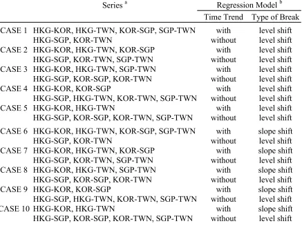
In Equation (3), we consider 10 cases. These are listed in Table 2. The results of

the Fisher_B test in those cases are presented in Table 3. The results obtained under

Equation (6) are mainly discussed below. The Fisher_B test can significantly reject the

null hypothesis in nine cases under the assumption of one break and in three cases under

the assumption of two breaks. Taking into consideration these significant results does

not reveal the apparent difference in the growth patterns across the economies; therefore,

consistent implications can be obtained from the most reliable results among them in

terms of the rejections at the lowest significant level, which are CASE 8 and CASE 10

under the one-break assumption. The common growth strategies examined in both cases

imply that the pair-wise growth experiences of Hong Kong–Korea and Hong

Kong–Taiwan represent a catching-up process; those of Hong Kong–Singapore and

Korea–Taiwan represent long-run convergence. In other words, Hong Kong and

state of long-run convergence between them, both Korea and Taiwan have been chasing

Hong Kong by narrowing the relative gaps in their per capita real outputs over the

sample period. With regard to the relationships between Hong Kong–Korea and Hong

Kong–Taiwan, if the estimates of the coefficients obtained from individual regression

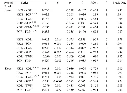
(shown in Appendix (Table 2A)) are evaluated with respect to their signs and values, the

existence of the catching-up phenomenon is also supported for these pairs of

economies.9 With regard to the case of a one-time slope shift, each of the difference

series, calculated by subtracting Korea or Taiwan’s logarithm of per capita real output

from that of Hong Kong, has the positive estimate of a constant (α ) and the negative

estimate of the slope of a time trend (β). The signs of these estimates imply that there

exists the initial gap of outputs between the two economies; however, this gap has been

decreasing at a constant speed over time. In other words, the gap suggests the existence

of the catching-up phenomenon. In addition, in the difference series for each pair of

economies, the estimate of δ —which is the coefficient of the dummy variable for the

slope shift—is also negative and its absolute value is much larger than that of β. This

suggests that the speed of catching-up was dramatically accelerated at a break date. In

other words, Korea and Taiwan have been catching-up with Hong Kong at a speed that

was accelerated after 1985 and 1990 respectively.

The fact that both CASE 8 and CASE 10 also imply long-run convergence between

Korea and Singapore is inconsistent with the findings described above. Moreover, the

categorization of the bilateral relations between Singapore and Taiwan is different in

these cases. The discussion under Equation (6) is also supported in the case of Equation

level for the one-break model under this DGP. This additional case suggests the

existence of a catching-up process between Korea and Singapore; however, this is not

conclusive.10

IV. CONCLUSION

This paper has examined the convergence hypothesis of per capita real output in the

Asian NIEs by applying the panel-based unit root test permitting multiple shifts in level

or slope at various unknown dates for each time series. Since the test also allows for

flexible specifications in terms of the presence or absence of a linear time trend and the

types of breaks (shifts in level or slope) for each series, different growth patterns across

economies have been investigated simultaneously.

The empirical analysis revealed the following facts: Although the long-run growth

paths of the Asian NIEs were shifted due to one or two external shocks, Hong Kong and

Singapore have been on the path of long-run convergence, while Korea and Taiwan

have been catching-up with Hong Kong, maintaining their bilateral relations,

characterized by long-run convergence. For the pairs of Korea–Singapore and

REFERENCES

Asian Development Bank (1998) Asian Development Outlook 1998, Manila: Asian

Development Bank.

Asian Development Bank (1999) Rising the Challenge in Asia: A Study of Financial

Markets: Volume 1 – An Overview, Manila: Asian Development Bank.

Barro, R. J. (1991) Economic growth in a cross section of countries, The Quarterly

Journal of Economics, 106, 407-443.

Bernard, A. B. and Durlauf, S. (1995) Convergence in International Output, Journal of

Applied Econometrics, 10, 2, 97-108.

Evans, P. (1998) Using Panel Data to Evaluate Growth Theories, International

Economic Review, 39, 2, 297-309.

Evans, P. and Karras, G. (1996) Convergence revisited, Journal of Monetary Economics,

37, 249-65.

Fisher, R. A. (1932) Statistical Methods for Research Workers, Oliver & Boyd,

Edinburgh, 4th Edition.

Hooi, L. H. and Smyth, R. (2007) Are Asian real exchange rates mean reverting?

Evidence from univariate and panel LM unit root tests with one and two structural

breaks, Applied Economics, 39, 2109-20.

Kim, J. U. (2001) Empirics for Economic Growth and Convergence in Asian

Economies: A Panel Data Approach, Journal of Economic Development, 26, 49-59. Kim, J.-I. and Lau, L. J. (1996) The Sources of Asian Pacific Economic Growth, The

Canadian Journal of Economics, 29, S448-54.

Lee, K., Pesaran, M. H. and Smith, R. (1997) Growth and convergence in a

multi-country empirical stochastic Solow model, Journal of Applied Econometrics,

12, 357-392.

Li, Q. and Papell, D. (1999) Convergence of international output: Time series evidence

for 16 OECD countries, International Review of Economics and Finance, 8, 267-80.

Lim, L. K. and McAleer, M. (2004) Convergence and Catching Up in ASEAN: A

Comparative Analysis, Applied Economics, 36, 137-53.

Lumsdaine, R. L. and Papell, D. H. (1997) Multiple Trend Breaks and the Unit-Root

Hypothesis, The Review of Economics and Statistics, 79, 212-8.

Maddala, G. S. and Wu, S. (1999) A Comparative Study of Unit Root Tests with Panel

Data and a New Simple Test, Oxford Bulletin of Economics and Statistics, Special

Issue, 631-52.

Matsuki, T. and Usami, R. (2008) China’s Regional Convergence in Panels with

Multiple Structural Breaks, Applied Economics, forthcoming.

McCoskey, S. K. (2002) Convergence in Sub-Saharan Africa: a nonstationary panel data

approach, Applied Economics, 34, 819-29.

Ng, S. and Perron, P. (1995) Unit root tests in ARMA models with data-dependent

methods for the selection of the truncation lag, Journal of American Statistical

Association, 90, 268-281.

Oxley, L. and Greasley, D. (1995) A Time-Series Prospective on Convergence: Australia,

UK and US since 1987, The Economic Record, 71, 259-70.

Credit, and Banking, 33, 804-12.

Young, A. (1995) The Tyranny of Numbers: Confronting the Statistical Realities of the

East Asian Growth Experience, Quarterly Journal of Economics, 110, 641-80. Zivot, E. and Andrews, D. W. K. (1992) Further Evidence on the Great Crash, the

Oil-Price Shock, and the Unit-Root Hypothesis, Journal of Business & Economic

FOOTNOTES

1. Krugman (1994), Young (1995), Kim and Lau (1996), and others discussed the

sources of their rapid economic growth from the 1980s to the mid 1990s.

2. For income convergence among countries, Li and Papell (1999) examined the

existence of convergence among 16 OECD countries by applying the univariate unit

root test with one endogenous trend break; using the panel unit root tests and panel

cointegration tests, McCoskey (2002) investigated whether a convergence club is

formed in sub-Saharan African countries.

3. Hooi and Smyth (2007) used the univariate and panel versions of Lagrange multiplier

(LM) unit root test that can treat two structural breaks in investigating the validity of

the purchasing power parity hypothesis in 15 Asian countries.

4. Beginning with li =8, the value of li is reduced one by one until aˆ is estimated il

to be different from zero at the 10% significance level.

5. Catching-up is intuitively comprehensible if the signs of αˆ_i and βˆ_{i are opposing,}

0 ˆ_i >

α and βˆi <0 or αˆi <0 and βˆi >0, although a particular account has not been

provided in Oxley and Greasley (1995) and Lim and McAleer (2004).

6. The MW test is built by applying Fisher’s p-value combination method to N

augmented Dickey-Fuller t-tests; therefore, it does not allow for breaks.

7. When error terms are correlated in DGP across a cross-sectional unit i, the Fisher_B

test does not have a chi-square distribution under the null because the minimum

i

t -tests are also correlated across i. Thus, without any correction, the test might

possess biases towards over- or under-rejections of the null. In order to correct these

(2001) resampling scheme, the empirical distribution function of the Fisher_B test is

generated through simulation. The simulation provides the appropriate small-sample

critical values for the test; these will be shown in Table 1A. Based on these critical

values, the test is conducted in an appropriate manner.

8. Formally, Alan Heston, Robert Summers and Bettina Aten, Penn World Table Version

6.2, Center for International Comparisons of Production, Income and Prices at the

University of Pennsylvania, September 2006.

9. The estimation results for each series in the case of two-time breaks are available on

request.

10.Under Equation (6), if CASE 6 and CASE 7, which are significant at the 5%

significance level in the case of one-break model, are added to facilitate the

interpretation, the relation between Korea and Singapore may also be traced to the

DGP Model Regression Model

(5) constant & trend 16.477 16.357 20.407 * constant 16.893 17.969 15.208

(6) a constant & trend 17.062 14.736 15.209 constant 19.060 21.225 * 18.231

* denotes statistical significance at the 10% level.

a

In the case of cross-sectionally dependent errors in the DGP, the critical values of the MW test and the Fisher_B test are tabulated in Table 1A in Appendix.

Table 1. The results for the Maddala and Wu (1999) test and the Fisher_B test in the case of shifts in level

MW test Fisher_B test

Series a

Time Trend Type of Break

CASE 1 HKG-KOR, HKG-TWN, KOR-SGP, SGP-TWN with level shift

HKG-SGP, KOR-TWN without level shift

CASE 2 HKG-KOR, HKG-TWN, KOR-SGP with level shift

HKG-SGP, KOR-TWN, SGP-TWN without level shift

CASE 3 HKG-KOR, HKG-TWN, SGP-TWN with level shift

HKG-SGP, KOR-SGP, KOR-TWN without level shift

CASE 4 HKG-KOR, KOR-SGP with level shift

HKG-SGP, HKG-TWN, KOR-TWN, SGP-TWN without level shift

CASE 5 HKG-KOR, HKG-TWN with level shift

HKG-SGP, KOR-SGP, KOR-TWN, SGP-TWN without level shift

CASE 6 HKG-KOR, HKG-TWN, KOR-SGP, SGP-TWN with slope shift

HKG-SGP, KOR-TWN without level shift

CASE 7 HKG-KOR, HKG-TWN, KOR-SGP with slope shift

HKG-SGP, KOR-TWN, SGP-TWN without level shift

CASE 8 HKG-KOR, HKG-TWN, SGP-TWN with slope shift

HKG-SGP, KOR-SGP, KOR-TWN without level shift

CASE 9 HKG-KOR, KOR-SGP with slope shift

HKG-SGP, HKG-TWN, KOR-TWN, SGP-TWN without level shift

CASE 10 HKG-KOR, HKG-TWN with slope shift

HKG-SGP, KOR-SGP, KOR-TWN, SGP-TWN without level shift

Table 2. The cases of the series and the regression models

Regression Model b

a

HKG, KOR, TWN, and SGP denote Hong Kong, Korea, Taiwan, and Singapore, respectively.

b

DGP Model CASE a

(5) 1 23.539 ** 19.394 * 23.836 **

2 19.964 * 20.362 * 23.707 ** 3 20.060 * 20.060 * 24.733 ** 4 18.773 * 19.550 * 15.971

5 17.957 21.028 * 24.604 **

6 - 23.859 ** 16.479

7 - 27.084 *** 17.395

8 - 27.168 *** 16.945

9 - 20.166 * 14.450

10 - 30.393 *** 17.860

(6) b 1 24.367 ** 18.390 18.987

2 21.132 * 19.797 * 19.171 * 3 22.697 ** 19.675 * 20.733 * 4 20.435 * 19.614 * 14.226 5 19.746 * 21.479 * 20.825 *

6 - 22.074 ** 15.194

7 - 26.055 ** 16.680

8 - 26.406 *** 15.649

9 - 20.283 * 14.365

10 - 30.122 *** 17.163

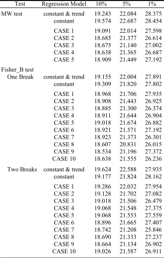
Table 3. The results for the Maddala and Wu (1999) test and the Fisher_B test in the ten cases

***, **, and * denote statistical significance at the 1%, 5%, and 10% levels, respectively.

b

In the case of cross-sectionally dependent errors in the DGP, the critical values of the MW test and the Fisher_B test are tabulated in Table 1A in Appendix.

a

See the cases of the series and the regression models in Table 2.

One Break Two Breaks Fisher_B test

Test Regression Model 10% 5% 1%

MW test constant & trend 19.243 22.084 28.375

constant 19.574 22.687 28.454

CASE 1 19.091 22.014 27.598

CASE 2 18.685 21.377 26.614

CASE 3 18.675 21.140 27.002

CASE 4 18.638 21.365 26.687

CASE 5 18.909 21.449 27.192

Fisher_B test

One Break constant & trend 19.155 22.004 27.891

constant 19.309 21.820 27.802

CASE 1 18.968 21.706 27.935

CASE 2 18.908 21.443 26.925

CASE 3 18.885 21.300 26.374

CASE 4 18.911 21.644 26.904

CASE 5 19.018 21.674 26.882

CASE 6 18.921 21.571 27.192

CASE 7 18.923 21.373 26.301

CASE 8 18.607 20.831 26.015

CASE 9 18.534 21.196 27.372

CASE 10 18.638 21.555 26.236

Two Breaks constant & trend 19.624 22.588 27.935

constant 19.177 21.824 28.162

CASE 1 19.286 22.032 27.954

CASE 2 19.128 21.702 27.082

CASE 3 19.018 21.506 26.479

CASE 4 19.068 21.548 27.375

CASE 5 19.068 21.553 27.559

CASE 6 18.896 21.665 27.407

CASE 7 18.742 21.208 25.846

CASE 8 18.690 21.333 27.237

CASE 9 18.664 21.134 26.902

CASE 10 19.026 21.587 26.911

Series α β φ δ Min t l _{Break Date}

Level HKG - KOR 0.236 -0.248 -0.107 -3.429 1 1993

HKG - SGP 7, 8, 10 0.032 -0.268 -0.036 -4.293 1 1994

HKG - TWN 0.145 -0.195 -0.085 -2.564 0 1994

KOR - SGP 8, 10 -0.352 -0.384 0.139 -4.349 4 1984

KOR - TWN 7, 8, 10 -0.092 -0.441 0.031 -4.474 1 1989

SGP - TWN 7, 10 0.253 -0.355 -0.100 -4.602 1 1983

HKG - KOR 0.662 -0.016 -0.555 0.158 -4.919 6 1979

HKG - SGP 0.014 0.001 -0.334 -0.070 -4.288 1 1994

HKG - TWN 0.270 -0.002 -0.314 -0.077 -3.932 0 1994

KOR - SGP -0.469 0.002 -0.484 0.118 -4.763 1 1984

KOR - TWN -0.090 -0.001 -0.509 0.061 -4.680 1 1987

SGP - TWN 0.429 -0.003 -0.546 -0.085 -4.937 1 1984

Slope HKG - KOR 7, 8, 10 0.943 -0.001 -0.939 -0.024 -5.723 4 1985

HKG - SGP 0.014 0.001 -0.318 -0.008 -4.058 1 1993

HKG - TWN 7, 8, 10 0.784 -0.004 -0.942 -0.021 -5.795 4 1990

KOR - SGP 7 -0.355 -0.0003 -0.383 0.007 -3.348 1 1974

KOR - TWN -0.079 -0.001 -0.438 0.003 -3.858 1 1983

SGP - TWN 8 0.501 -0.072 -0.450 0.067 -3.994 1 1963

7, 8, and 10 denote the series used in CASE 7, CASE 8, and CASE 10, respectively. Type of

Break