An Association Rule Mining for Materialized View
Selection and View Maintenance
P.R. Vishwanath
Associate Professor CSE, RITS Hyderabad
Rajyalakshmi
Professor CSE,JNTUK Vizaynagaram
Sridhar Reddy
Professor Principal,SCET
Hyderabad
ABSTRACT
Data warehouse (DW) is a repository with query interface in support of Decision support systems. DW required answering many complex queries, managerial level queries and analytical queries, needing to develop advanced computing techniques. The DW system process involving data modeling, ETL process, query interface and reporting system. Materialized views (MV) are the pre calculated views which are used to increase the DW system performance. MV selection and maintenance need to adopt new trends and techniques. Data mining (DM) is the process of extracting hidden useful information from huge data bases .Literature of Data Mining (DM) involving algorithms and techniques related to association, classification and clustering. Recent researches shown Data mining can also be used in optimization of calculating MV‟s. In addition to DM techniques are also used in efficient calculation of Data cubes. This paper proposed frequent rule mining on of the Data mining approach for the selection and maintenance of MV‟S. By using the advanced concepts of frequent mining algorithm the query response time can be decreased. The approach also combines the advanced techniques to accommodate the changes in updating the base data so as to increase the performance of existing MV‟S selection and maintenance approaches.
Keywords
Data warehouse, Data mining, Data cubes, DW Maintenance, Clustering.
1.
INTRODUCTION
According to W H Inman data warehouse is a subject-oriented, integrated, nonvolatile and Time-variant collection of data in support of management‟s decisions [1]. The tasks of data warehouse are data cleaning, data integration, data consolidation and summarization. Data warehouse uses the update driven approach rather than query driven approach in which data from multiple heterogeneous sources is integrated in advance and stored in a warehouse/repository for direct querying and analysis. Different Data warehouse tools are used at different levels such as data modeling tools, ETL tools, Multi-dimensional data base tools, reporting and analysis tools.
Data warehouse backend tools include function such as Data extraction, Data cleaning, Data transformation, Load and refresh. As the Data warehouse contains huge volumes of historical data OLAP technology demands the queries to be answered in span of seconds. It requires efficient multidimensional models such as cube technology, access methods and query processing techniques to decrease the work load on Data warehouse system. This paper uses partial materialization to decrease the storage and quick response time.
Data mining refers to extracting hidden useful knowledge from large amounts of data. The tasks of data mining are characterization, association, classification, and clustering and outlier analysis. Data mining has become an important tool in information technology as huge amount of data is converted into useful information and knowledge. Number of algorithms and approaches on each task on data mining are developed these algorithms are used in different applications such as medical, clinical, banking and communication. These algorithms are also used in improving the performance of data warehouse (Data warehouse maintenance).
The paper is organized as Follows: Section 2 explains about data warehouse, data mining and materialized views. Section 3 explains the existing algorithms and approaches to find materialized views and usage of the different algorithms used in MV selection and MV maintenance. Section 4 explains the approach, proposed algorithm, framework and architecture of the presented and proposed algorithms. Section 5 explains about Cost Function. Section 6&7 explains the experimental results and comparison with the existing algorithms. Section 8 explains conclusion and future enhancements.
2.
LITERATURE REVIEW
2.1 Data Warehouse
According to Inman Definition Data warehouse is a subject oriented, time variant, nonvolatile and integrated collection of data in support of Decision support system [1]. Data warehouse technology includes data cleaning, data integration and online analytical processing. OLAP tools support multidimensional analysis and decision making. Relational data base model uses entity relationship model and schema contains set of entity and relationships between them. Popular Data Model for a data warehouse is multi-dimensional data model. Multi-dimensional data model is in the form of star schema, snow flake schema or a fact constellation schema. In the above most popular one is Star schema which contains central table known as fact table containing bulk of the data with redundancy and dimension tables for each direction.
2.2
Data Mining
Data mining refers to extracting hidden information or knowledge from large amount of data. Data mining (DM) is also known as knowledge discovery from data (KDD). KDD involving following steps 1) Data cleaning 2) Data integration3)Data selection4)data transformation 5)Data mining 6) Pattern evaluation 7)Knowledge presentation. Data is input for the DM system and Interesting pattern is the output. Data mining functionality involve concept or class description. The data is associated with classes or concepts which is useful to describe classes and concepts in summarized concise and precise way which is achieved via data characterization data discrimination, Statistical measures and plots, OLAP rollup operations, Attribute oriented induction.
Mining frequent patterns, Associations and correlation: Mining frequent patterns involves finding a frequent item set, frequent occurring subsequence etc. Frequent item set mining involved finding Associations and correlations in data. The Data mining algorithms developed to find associations are Apriori algorithm, FP GROWTH algorithm etc.
Classification and prediction: Classification is the process of finding a model that describes and distinguishes data classes or concepts .The process involving finding decision tree or a set of rules or a neural network. Algorithms developed to find classifiers are ID3, C4.
Cluster Analysis: Clustering methodology in DM divides the given data into groups or cluster based on their similarity. Algorithms developed related to clustering are means, k-medoids etc.
Outlier Analysis: Generally some part of the data or data objects behavior do not comply with the model of the data finding such data is known as Outlier Analysis.
Evolutionary Analysis: Behavior of the data changes over time this type of data needs separate mechanism which is known as Evolution Analysis
2.3
Materialized Views
Materialized views comprise pre computed and summarized information with the aim of answering most queries posed on data warehouse thereby saving of query processing time and storage. With the increase of attributes in each dimension there is need of increase of pre calculation of MVs. In this regard there is the increase of work load, needs to decrease the response time and storage. There are many view selection algorithms proposed. Continuous updating in the base table is to be reflected in the dimension a table, as the information is in DW is in the form of Fact. It is not possible to change whole DW instead changes to be accommodated at only affected part of DW. For this updating many views maintenance algorithms are proposed.
3.
EXISTING APPROACHES
4. PROPOSED ALGORITHM
In this approach the set of SQL statements considered as workload which is selected to configure materialized views for partial materialization. This approach of ARMMVVM has two parts materialized view selection (MVS) and Materialized view maintenance (MVM) algorithms. The first step is to transform set of SQL statements into transactional data base. Apriori rule mining algorithm is applied on the transactional database to get frequent Item sets. The transactions not holding the frequent sets are eliminated and the remaining transactions are then transformed to respective queries. The resultant queries are Partial MVs set to be calculated. Finally updation process is applied to these MVs to get MVs updated. Consider the attributes in the base relation are {a1, a2
...an}.Consider the workload i.e. Set of SQL statements
previously posed are {Q1, Q2, Q3 …Qr}. {ai1, ai2,
ai3……….aij} are the attributes present in the query Qi. Each
Qi transformed to transaction Ti by taking the attributes in it.
The set of all Ti‟s form the transactional Database. Applying
the MVS algorithm on this Transaction Data base we get reduced set of Ti‟s. This set is transformed to the set of Qi„s
which is the reduced work load.
In the query I such as SELECT sales.time_id, sum (quantity_sold), sum (amount_sold) from SALES, TIMES where sales.time_id = times.time_id and times.fiscal_year in (1998, 2000) group by sales.time_id . The transaction with respect to Qi is Ti represented as Ti: time_id, fiscal year. The Association mining called Apriori algorithm is used to find Association rules so as to get frequent item sets.
4.1 Materialized View Selection (MVS):
Step 1: Q the set of queries QiStep 2: Transform Qi to Transactions/Items Ti
Step 3: Apply Apriori algorithm on T= {T1, T2,... Tr} to get
frequent Item Sets.
Step 4: Find the T1 the set of transactions containing the frequent item sets.
Step 5: Find Q1 from T1
Step 6:Q1 is the required Selection of Materialized Views (partial) from Q (Total).
Apriori algorithm is applied on the transactional database T= {T1,T2,T3……..Tr} to get best association rules on this
transactional data bases. Rule 1,Rule 2…Rule j are the rules used find frequent item sets .Each rule finds the transactions holding these frequent item set .In this process the transactions not holding any frequent item set are eliminated. The transaction set {Tk1, Tk2….Tkp} (1≤kp≤r) remained are
the resultant transactional data base as the output on applying apprioi algorithm. Next to find the respective queries set {Qk1,Qk2…..Qkp} from{Tk1,Tk2….Tkp} (1≤kp≤r). These
queries are now calculated and considered for configured set of MVs. This enhanced Architecture deducted 27% of the queries from the given work load of 61 Queries. Fig 1 shows the frame work for proposed work
The above ARMMVS algorithm reduces the workload. After the Selection of MV‟s by above algorithm there may be changes in the base relations due to the updations in base table. These updations are to be reflected in the views selected in above reduced workload. This paper presents the Updation process in addition to the above process as part of View Maintenance. Updation process is used to the configured workload. Each Updation is recorded as one query. These
Queries are transformed as transaction TDi. Each TDi contains
attributes as in ARMVS algorithm.
Fig1: Frame work for MVS and MVM
4.2 Materialized View Maintenance (MVS):
Qi: The query containing some or all attributes from set ofattributes from {a1.a2…..an}.
Ti: The set of attributes {aij} Corresponding to Qi for i=1,
2,…r. and aij €{as} for some 1≤s ≤n and for some 1≤ j ≤ n
i.eT1={a11,a12,….a1s},Ti={ai1,ai2,…aij}
D: The set of all updated queries.
TD: The set of all attributes Contained in queries in D TD= {TD1, TD2 ,……TDt} where TDx= {ap} for Some p(1≤
p≤ n)
Ql: The set of reduced work load by MVS algorithm Tl: The set of Transactions corresponding to Ql We construct DTl using step2 of following algorithm
Step1: Input T1 and TDx
Step2: For i=1, 2… r, aij∈Ti,TDx∈TD
Ti ∈DT1
if aij∈TDx for 1≤x≤t and
for 1≤j≤ n Ti ∉DT1
otherwise.
Step3: DTl is the set of transactions from Tl. Corresponding to each element in DTl we get a Query in Ql. Therefore DQ1 is the set of Queries which is a part of Ql
Step4: DQ1 is the set of queries to be pre-calculated from Q1. In the above MVM algorithm, set of transactions TDi
considered as TD. Further each transaction in TD is compared with the each transaction in the Tl of MVS algorithm. By
algorithm. Finally the MVM algorithm gives the output DQl which is the subset of Q1of MVS algorithm. This DQl
required to be recalculated instead of recalculating all the queries in Ql with the effect of updation of values of attributes in base tables.
5. COST MODEL
We use the cost model in which the cost of answering the query is assumed to be equal to the number of tuples in the aggregate used to answer the query. Our experiments show that there is a linear ship between sizes and running time of query. The cost of answering a query q is equal to the number tuples read to return the answer. We introduced THE GAIN MEASURE (GM) to measure the gain from work load to the resultant queries.
5.1 The Gain Measure
The gain measure of an aggregate view s is computed by adding up the saving in query cost for each view t, including
s, over answering from the base view. If a set D of aggregated views is chosen for materialization, the gain of D is the sum of the gain of all views in D. We now calculate the gain of an aggregate view. If D is a set of aggregates that have already been selected for pre computation, the gain of views is concerned with how materializing s improves the cost of computing other views, including it. Let C(s) be the cost of computing another view from s. looking back to our cost model C(s), is the number of tuples in s. The gain of s with respect to the D. G(s, D) is defined as follows
1. For each aggregate view s ≤ t ,G(s) defined as a) Let r be the least cost view in D such that s ≤ r
b) If C(t)<C(r) the G(s)= C(r)- C(t) ,else G(s)=
0
2. G(s ,D )= 𝒔<𝑡 𝑩(𝒔)
Precisely, for each view s that is a descendant of t, we check to see if computing s from sis cheaper that computing s from any other view in the set D. If this is the case, then pre computing t gains s. Since all aggregates can be computed from the (un-aggregated) base data, in step 1(a) we can always find a least cost aggregate view r. Using Gain Measure two approaches ARMMVVM and CBMVS are compared and results are presented in fig 6.
6. EXPERIMENT AND RESULTS
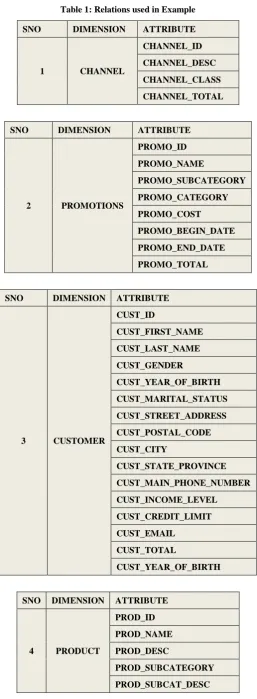
In order to verify proposed framework for MV selection and maintenance use of the work load containing sixty one data warehouse queries is required. The queries taken from http://eric.univ-lyon2.fr/~kaouiche/adbis.pdf.Tests are carried on up to 2 GB data warehouse using the Data base oracle .A system with configuration Pentium Core to Duo PC with 2 GB RAM and a 500GB hard disk. This Data Warehouse contains five dimension table and one fact tables. Dimension tables are PRODUCTS, TIMES, CHANNELS, PROMOTIONS, CUSTOMERS.PRODUCTS table containing 15 attributes, CHANNELS table containing 4 attributes, PROMOTIONS table containing 8 attributes, CUSTOMERS table containing 15 attributes and TIMES table containing 31 attributes. FACT table is SALES. SALES containing quantity sold, amount sold as two facts.
[image:4.595.300.558.68.769.2]Table 1 show the Dimension tables used from the Popular Schema known as Star Schema.
Table 1: Relations used in Example
SNO DIMENSION ATTRIBUTE
1 CHANNEL
CHANNEL_ID
CHANNEL_DESC
CHANNEL_CLASS
CHANNEL_TOTAL
SNO DIMENSION ATTRIBUTE
2 PROMOTIONS
PROMO_ID
PROMO_NAME
PROMO_SUBCATEGORY
PROMO_CATEGORY
PROMO_COST
PROMO_BEGIN_DATE
PROMO_END_DATE
PROMO_TOTAL
SNO DIMENSION ATTRIBUTE
3 CUSTOMER
CUST_ID
CUST_FIRST_NAME
CUST_LAST_NAME
CUST_GENDER
CUST_YEAR_OF_BIRTH
CUST_MARITAL_STATUS
CUST_STREET_ADDRESS
CUST_POSTAL_CODE
CUST_CITY
CUST_STATE_PROVINCE
CUST_MAIN_PHONE_NUMBER
CUST_INCOME_LEVEL
CUST_CREDIT_LIMIT
CUST_EMAIL
CUST_TOTAL
CUST_YEAR_OF_BIRTH
SNO DIMENSION ATTRIBUTE
4 PRODUCT
PROD_ID
PROD_NAME
PROD_DESC
PROD_SUBCATEGORY
PROD_CATEGORY
PROD_CAT_DESC
PROD_WEIGHT_CLASS
PROD_UNIT_OF_MEASURE
PROD_PACK_SIZE
SUPPLIER_ID
PROD_STATUS
PROD_LIST_PRICE
PROD_MIN_PRICE
The queries are first transformed in to the transactional Data bases. The attributes present in each query are identified as transactional items. Each Qi in the figure represents one corresponding transaction Ti in Transaction data base. Figure 3 shows the present Query transaction table. D= {T1, T2 ,…..T60,T61} are the given transaction database as input to the Apriori algorithm. The best rules are found by the Apriori algorithm and from them the frequent item sets found are {PROMO_ID,PROMO_CATEGORY},{PROMO_CATEGO RY, PROD_ID}, {CUST_ID, CUST_GENDER}, {PROD_ID, PROD_CATEGORY}. From these Frequent Item sets transactions eliminated. The remaining Transactional Data base is given by {T2,T3, T4,T5,T10,T10,T13,T16,T17,T18,T19,T21-T25,T29,T33-50,T52,T54-T61}. Then our workload reduced to {Q2,Q3,Q4 ,Q5,Q10 ,Q10,Q13,Q16, Q17,Q18,Q19,Q21-Q25,Q29,Q33-Q50,Q52,Q54-Q61},which has 45 queries for calculating MV‟s. Finally the updated queries resulted changes in attribute values of base table are taken. These queries are then transformed to transactions set by considering their attributes present in each updated queries. The elements are compared with the above 45 Transactions of output of MVS algorithm. T2, T29, T52 are the transactions as the output of MVM algorithm. There by MVM algorithm concludes Q2, Q29, and Q52 which requires re-computation so as to reflect updated queries on Base tables. The experiment is continued by generating the Transactional database of 1GB, 5GB, 10 GB, and 15 GB. Applying ARMMVVM approach more gain is obtained than CBMVS approach.
7. COMPARISIONS
[image:5.595.54.279.71.225.2]Fig 2 shows the number of queries taken and the output after applying presented ARMMVVM algorithm. First taken 61 queries and increased up to 200 queries. The chart shows the reduced workload in each case .As Fig 6, shown the efficiency of the approach increases with the increase of the work load.
Fig 2: Reduced work load using ARMMVVM
Fig 3 shows the comparison between the CBMVS algorithm and ARMMVVM in each case by increasing the number of queries as in Fig 6. It is shown 10% to 20% reduced workload by using ARMMVVM algorithm. It shows that the ARMMVVM approach presented in the paper is better than CBMVS algorithm.
Fig 3: Comparison between ARMMVVM and CBMVS algorithm
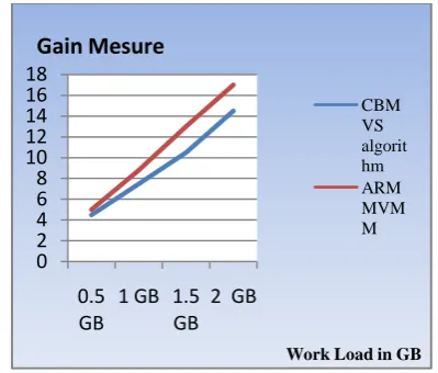
Fig 4 shows the comparison between the CBMVS algorithm and ARMMVVM using the proposed GAIN MESURE. It is found by experiments that the Gain using the ARMMVVM is more than CBMVS algorithm.
Fig 4: The comparison between ARMMVVM and CBMVS algorithm using Gain measure.
8. CONCLUSION AND FUTURE
WORK
Data warehouse is the backend process for business analytics. With the dynamics in Analytics in reporting, the challenges are increasing day by day in Data ware house systems. Calculating the Appropriate MV‟s is the challenge in the DW research area. This paper presented the Association rule mining one of the Data mining technique used for improving the performance of the MV selection and MV maintenance. This Approach uses novel approach to find partial materialized views from the materialized views. Results of the approach show ARMMVVM is efficient when compared from the existing approaches and makes use of the data mining technique. This work can be extended by considering the fact table in rule mining for MV selection. Future work also extended to consider concept hierarchies for each Dimension.
0 50 100 150 200
250 worklaod
Selection of MV's using ARMMVV M
INPUT WORK LOAD
OUTPUT WORK LOAD
0 50 100 150 200 250
1 2 3 4
workload
ARMM VVM
INPUT QUERIES
OUTPUTQUERIES
0 2 4 6 8 10 12 14 16 18
0.5 GB
1 GB 1.5 GB
2 GB
CBM VS algorit hm ARM MVM M
Gain Mesure
[image:5.595.317.541.141.288.2] [image:5.595.327.527.362.532.2] [image:5.595.57.261.625.743.2]9. REFERENCES
[1] W. Inmon, “Building the data warehouse”, Wiley publications, pp 23, 1991.
[2] Jiawei Han and MichelineKamber , “Data Mining Concepts and Techniques, 2nded.Morgan Kaufmann
Publishers, March 2006. ISBN 1-55860-901-6
[3] Nalini, T, Kumaravel, A and Rangarajan, K ,”A Novel Algorithm With Im-Lsi Index For Incremental Maintenance Of Materialized Views”.Proceedings of JCS&T Vol. 12 No. 1, April 2012SOURCE
[4] An Gong, Weijing Zhao, “Clustering-based Dynamic Materialized View Selection Algorithm” Proceedings of Fifth International Conference on Fuzzy Systems and Knowledge Discovery, 2008, China,pp391-395
[5] K.Aouiche, P.EmmanuelJouve, and J.Darmont ,“Clustering-Based Materialized View Selection in Data Warehouses”TechnicalReport, University of Lyon 2, 2007.
[6] T.Nalini,Dr. A.Kumaravel, Dr.K.Rangarajan ,” An Efficient I-Mine Algorithm For Materialized Views In A
Data Warehouse Environment”, Ijcsi International Journal Of Computer ScienceIssues, Vol. 8, Issue 5, No 1, September 2011 Issn (Online):1694-0814
[7] D. Xin, J.Han, X. Li, and B.W.Wah. Star-cubing: Computing iceberg cubes by top-downand bottom-up integration. In Proc. 2003 Int. Conf. Very Large Data Bases (VLDB‟03),Berlin, Germany, pages 476–487, Sept. 2003.
[8] T.V.Vijaykumar and KalyaniDevi,“Frequent queries identification for constructing materialized views”,Journal of Computer Science & Technology (JCS&T);2012, Vol. 12 Issue 1s, p32.
[9] Yogeshree D. Choudhari,Dr. S. K. Shrivastava “Cluster Based Approach for Selection of Materialized Views “ proceedings of International Journal of Advanced Research in Computer Science and Software Engineering (IJARCSSE)july2012
[10] P.R.Vishwanath Dr.D.Rajyalakshmi Dr.Sreedhar reddy “A Comparative Study of Data Mining Techniques in Maintenance of Data “, IJSER Volume 4, Issue 11, November 2013 Edition.